IEEE TRANSACTIONS ON SIGNAL PROCESSING, VOL. 56, NO. 6, JUNE 2008
2229
Target Tracking by Particle Filtering in Binary Sensor Networks Petar M. Djuric´, Fellow, IEEE, Mahesh Vemula, Student Member, IEEE, and Mónica F. Bugallo, Member, IEEE
Abstract—We present particle filtering algorithms for tracking a single target using data from binary sensors. The sensors transmit signals that identify them to a central unit if the target is in their neighborhood; otherwise they do not transmit anything. The central unit uses a model for the target movement in the sensor field and estimates the target’s trajectory, velocity, and power using the received data. We propose and implement the tracking by employing auxiliary particle filtering and cost-reference particle filtering. Unlike auxiliary particle filtering, cost-reference particle filtering does not rely on any probabilistic assumptions about the dynamic system. In the paper, we also extend the method to include estimation of constant parameters, and we derive the posterior Cramér-Rao bounds (PCRBs) for the states. We show the performances of the proposed methods by extensive computer simulations and compare them to the derived bounds. Index Terms—Binary sensor networks, particle filtering, posterior Cramér-Rao bounds (PCRBs).
I. INTRODUCTION ECENT advances in low-power micro sensors, actuators, embedded sensors, radio, and in general, digital wireless communication technologies have allowed development of wireless sensor networks with unparalleled capabilities [5]. Their use may span a vast range of fields, and their effectiveness is already being felt both in commercial and military applications as well as in the further development of science and engineering [6], [14], [24], [30]. In this paper, we consider wireless sensor networks with two basic components, sensors and a fusion center. The sensors sense and measure signals that provide information about an event or events of interest and send binary information to the fusion center. The fusion center combines the received information to obtain estimates about the observed phenomenon. Here the object of interest is a single target that moves in a field of sensors that measure signal power, and the objective is the online estimation of its trajectory, velocity, and power. Often sensor networks have to operate with sensors that have limited power as well as limited communication and computational resources. At a strategic assessment workshop organized by the U.S. Army Research Lab it was concluded that [1]
R
Manuscript received October 6, 2006; revised October 31, 2007. This work was supported in part by the National Science Foundation under Awards CCF0515246 and by the Office of Naval Research under Award N00014-06-1-0012. The associate editor coordinating the review of this manuscript and approving it for publication was Dr. Venkatesh Saligrama. The authors are with the Department of Electrical and Computer Engineering, Stony Brook University, Stony Brook, NY 11794 USA (e-mail: djuric@ece. sunysb.edu;
[email protected];
[email protected]). Color versions of one or more of the figures in this paper are available online at http://ieeexplore.ieee.org. Digital Object Identifier 10.1109/TSP.2007.916140
“it is not practical to rely on sophisticated sensors with large power supply and communication [demands]. Simple, inexpensive individual devices deployed in large numbers are likely to be the source of the battlefield awareness in the future.” One type of networks that fits this description is the class of binary sensor networks, where the sensors transmit only binary information about sensed events (the event is sensed or is not sensed). The signals that reach the fusion center of these networks are therefore binary signals embedded in noise, and they pose challenging problems for recovering the sensed information by the sensors. The sensed information in this paper is the intensity (signal power) of the transmitted signals by one or more sources that attenuates as a function of distance from the sources.1 For the tracking we propose to apply the auxiliary particle filter (APF) [23] and the cost-reference particle filter (CRPF) [3], [16]. The two methods are sequential statistical signal processing procedures with distinct features but with similar algorithmic outline. Convergence properties of the particle filtering methods can be found in [8] and [19] and of the CRPF in [16] and [17]. The main contribution of the paper is in the application of the APF and CRPF on binary signals and in the presence of hidden complete measurements by the sensors. We show how the signals from the binary sensors contribute to producing evolving random grids of the methods, how the associated metrics of the grid nodes are updated, and how the estimates of the unknowns are obtained. We also outline the steps for computing the posterior Cramér-Rao bounds (PCRBs) of the state estimates. The paper is organized as follows. First, in Section II we provide a brief overview of the literature related to binary sensor networks. In Section III, we describe the binary sensor network and define the addressed problem in a mathematical form. In Section IV we present the APF and CRPF algorithms for tracking a single target. In the following section, we discuss extensions of the algorithms for the case of unknown emitted power. In Section VI we address the PCRBs of the tracked variables. Details of the derivation of the bounds are shown in the Appendix. Simulations that demonstrate the performance of the proposed methods are given in Section VII. We end the paper with Section VIII where we provide final remarks. II. A BRIEF LITERATURE SURVEY Binary sensors have already been addressed in the wide literature. In [15], a cooperative tracking method based on acoustic binary sensors was described. There, the tracking is based on a cooperative algorithm where the model of the target path is a 1We note that binary sensors of other sensing modalities can be used analogously along the lines presented in this paper.
1053-587X/$25.00 © 2008 IEEE Authorized licensed use limited to: SUNY AT STONY BROOK. Downloaded on April 30,2010 at 18:21:59 UTC from IEEE Xplore. Restrictions apply.
2230
IEEE TRANSACTIONS ON SIGNAL PROCESSING, VOL. 56, NO. 6, JUNE 2008
binary sensors that may be deThe network consists of ployed randomly, deterministically, or both. In all cases, we assume that the fusion center knows the locations of all the sensors and that the locations remain fixed for all time. B. Mathematical Models The model for target movement is standard and is described by [11] (1)
Fig. 1. A binary sensor with a target passing nearby. The signals transmitted by the sensors are denoted by s .
piece-wise linear curve and is different from the one that we use in our paper. In [2], as in this paper, a particle filteringtype algorithm for tracking was introduced. However, the authors focus on geometric properties of the sensors’ configuration and derive their algorithm based on that geometry. Also, the method is based on sensor data that provide information about approaching or receding targets with respect to the individual sensors, whereas in our approach we only use information about the proximity of the target to the sensor. In [12], a tracking method was proposed that first estimates the positions of a target in its most recent past and then fits them with a piece-wise trajectory. In [21], another method for distributed tracking in binary sensor networks was developed. It is derived by using hidden state estimation and the Viterbi algorithm. In other recent publications on signal processing for binary sensor networks, various problems have been addressed. For example, in [20] acoustic binary sensors were used for maximum likelihood localization (not tracking) of a source, and in [29] they were applied for system identification. Decentralized detection by binary sensors was presented in [4] where the sensors use a multiple access channel of limited capacity. Sufficient conditions were found that allow for minimal probability of error at the fusion center. III. NETWORK DESCRIPTION AND MATHEMATICAL MODELS A. Network Description In a binary sensor network, the deployed sensors measure a signal of interest and if the level of the measured signal is above a predefined threshold, they report to the fusion center with a signal that identifies them; otherwise they are silent. Their function is best described by a way of example. In Fig. 1, a binary sensor is represented by the small circle and its range by the larger circle. When the target is outside the range of the sensor, the received signal is below the set threshold, and the sensor does not transmit anything (instants , and ). During the time when the target is inside the range of the sensor, the received signal is above the threshold, and the sensor transmits a “one” to the fusion center (instants , , and ). When at a given time the fusion center does not receive a signal from a particular sensor, this implies that the sensor transmits a “zero.”
where is a state vector, which indicates the position and the velocity of the target in a two-diand are known mensional Cartesian coordinate system, matrices given by
with being the sampling period and , a 2 1 zero-mean vector representing the state noise process and which accounts for the acceleration of the target. The APF method uses an additional assumption about ; it is a Gaussian vector with a co. variance matrix The received power can be modeled as in [22] or as in [25]. We adopt the latter model, that is, the measurement of the th sensor is given by
(2) where is a function that models the received signal power by the th sensor; is a noise process independent from and independent from noise samples of other sensors; is the position of the th sensor; is the location denotes the Euclidean distance of the target at time ; between and ; is the emitted power of the target measured at a reference distance ; is an attenuation parameter that depends on the transmission medium and is considered to be known and the same for all sensors. For the application of the . In our model, we APF, we need to know the distribution of where with being assume that the known power of the background measurement noise of one , with being the number of samples sample and used to obtain the measured power [25]. For the CRPF, we only assume that we know . measures the received power The th sensor , processes it locally and transmits a single binary digit to the fusion center according to the following rule. , 1) The sensor compares the actual observed power level, with a threshold, . If the sensed value is below , it does not transmit anything. 2) If the sensed value is greater than , the sensor transmits its identification code to the fusion center. Therefore, the sensors in the network send signals to the fusion center only if the received power is greater than the sensor thresholds.
Authorized licensed use limited to: SUNY AT STONY BROOK. Downloaded on April 30,2010 at 18:21:59 UTC from IEEE Xplore. Restrictions apply.
´ et al.: TARGET TRACKING BY PARTICLE FILTERING DJURIC
2231
The received signal from the th sensor at the fusion center is modeled as
Since the noise samples dent, we have
from (3) are assumed indepen-
(3)
(6)
where if if
For the factors (4)
and where is the observation noise, and is a known attenuation coefficient associated with the th sensor. Again, for the APF method we need the knowledge of the noise distribution of , and we let , whereas for the CRPF method we only assume that the noise is zero mean. In summary, the measurements made by the sensors are complete and are modeled by (2). The sensors, however, always transmit binary signals constructed according to (4), and the fusion center receives them as quantified by (3). The objective is to track the evolving state using the observations , that is, the observations up to time instant of the first sensor, , the second sensor, , as well as the remaining sensors, . The APF uses probabilistic assumptions about all the noises in the model and about the prior of the states. The CRPF only needs knowledge of the first moments of the noises. IV. TRACKING ALGORITHMS First we present a tracking algorithm based on APF [10], [23] (Section IV-A), and then we proceed with the presentation of a CRPF algorithm [3], [16] (Section IV-B). In this section, the parameter is assumed known, but subsequently this assumption will be dropped. A. APF Algorithm Recall that according to the theory of particle filtering, we , , by aptrack the a posteriori distribution of proximating it with a random measure composed of particles and weights , where is an index, and which we dewith being the number of note by particles. At every time instant , the particle filter carries out the following operations: (1) Selection of most promising particle streams, (2) particle propagation, (3) computation of particle weights, and (4) state estimation. The APF attempts to draw from an importance function which is as close as possible to the optimal one. To that end, the selection of most promising particles is carried out by sampling from a multinomial distribution where the number of possible and the probabilities of the respective outcomes outcomes is are , , and (5) where .
is some parameter that characterizes
, we can write
given
(7) where (8) and (9)
(10) where denotes the complementary of the standard normal cumulative distribution function. , At the beginning, the initial set of particles , are drawn from a prior distribution , . Suppose now and the weights of the particles are set to , we have the random measure that at time instant . Then the steps of a particle filter recursion can be implemented as follows. 1) Selection of Most Promising Particle Streams: For selection of the most promising particles, we use the conditional given as a characterizing parameter of every mean of stream, i.e. (11) The conditional means are computed readily from (12) This is followed by computation of the weights according to (5) and their normalization. Finally, a set of indices are drawn from the probability mass function (pmf) represented by the normalized weights. 2) New Particle Generation: The first two elements of represent the location of the the four-dimensional state target in a two-dimensional space, and the remaining elements are the components of the velocity in this space. That implies that the generation of requires drawing only twodimensional random variables. The generation can be carried out by first, propagating the velocity components one step ahead using the joint distribution
Authorized licensed use limited to: SUNY AT STONY BROOK. Downloaded on April 30,2010 at 18:21:59 UTC from IEEE Xplore. Restrictions apply.
2232
IEEE TRANSACTIONS ON SIGNAL PROCESSING, VOL. 56, NO. 6, JUNE 2008
or locations according to
and second, computing the (13) (14)
The above equations are obtained from (1). 3) Weight Computation: The newly generated particles are assigned weights according to
The likelihood terms of the numerator and denominator are calculated as in the APF using (6)–(10). 4) State Estimation: Once the weights are normalized, one to compute estimates of the unknown states. If we can use want the minimum mean square error (MMSE) estimate, we obtain it from
The procedure has four steps: (1) selection of most promising particle streams, (2) propagation of particles, (3) cost update, and (4) state estimation. The initialization of the method is carried out by randomly drawing initial particles from some probwhose support includes the ability density function (pdf) space of . We propose that the method is implemented as follows. 1) Selection of Most Promising Particle Streams: This step is reminiscent of the main idea of the APF, where resampling takes place by using measurements from at time instant , time instant . For CRPF, we define a risk function which quantifies the quality of the particle given the next set of observations, . As a risk function, one can use the incremental cost, that is, in our case
with (18) (19)
(15)
(20) B. CRPF Algorithm The objective of CRPF is to estimate sequentially the evolution of the unknown state from without assumptions about the probability distributions of the noises in the model. It is similar in structure to that of the APF because CRPF, too, uses a discrete random measure. This random measure is composed of particles and costs associated to them, where the costs are user-defined. We denote the random measure by , where has the same meaning as are the associated costs to . It is clear before and that the costs here play the role of the weights in APF. In fact, with appropriate choices of the costs, one can make the CRPF equivalent to the APF or the standard particle filter [3]. In general, the costs are updated according to [16]
(16) , and where is a forgetting factor is an incremental cost. Obviously, the value of controls how fast the state estimates can adapt to new values of the states. The incremental cost contributes to the total cost at time instant and is a function of the particle value and the observation at that instant. A typical incremental cost has the form (17) is a function of , and . So, CRPF prowhere ceeds analogously to the APF; with the vector of observations , the discrete random measure at time instant , , is updated to to reflect accurately the possible value of the unknown state at time instant , .
where the elements of are defined by (2) and those of by (3) and (4), i.e., the elements of are given by
Once the risks are computed, they are added to their costs at to obtain the predicted costs, i.e. (21) The particles are then sorted according to their predicted costs in ascending order and the first of the particles are times (we assume that is an integer). In replicated other words, each of the surviving particles will have children at time instant [3]. We note that in previous versions of CRPF implementations we used functions to generate pmfs, where the latter were subsequently used for resampling of the particles. With the sorting scheme, we avoid the use of such functions and classical resampling and instead, we proceed directly with removing “bad” particles. Many simulation results have shown that with this simpler and faster scheme we do not sacrifice performance. 2) Particle Propagation: For particle propagation we can use a Gaussian proposal density in a similar way as is done with APF. Note that the functional form of the Gaussian is not used for computing the costs of the particles. Also, the use of a Gaussian is not required, and we can use any other density that is centered around the particle and that produces random variables with appropriate variance, like a uniform, or a Laplace, or a Cauchy density. If we use a Gaussian, we draw the velocities of the target with and with covariance matrix mean , where the s denote indexes of sorted particles,
Authorized licensed use limited to: SUNY AT STONY BROOK. Downloaded on April 30,2010 at 18:21:59 UTC from IEEE Xplore. Restrictions apply.
´ et al.: TARGET TRACKING BY PARTICLE FILTERING DJURIC
and
2233
’s are surviving particles from step 1. The variance, , is recursively updated by (see [16])
The locations are then obtained by (13) and (14). 3) Cost Update: The cost update is performed by using (16). 4) State Estimation: The state is estimated by using the particles and the associated costs. One way of carrying out the estimation is by creating a pmf from the costs. To that end, a monothat converts the set of costs tonically decreasing function is defined, that is into probability masses
One function that has worked well for different problems is
Once the , are computed, the estimation can be carried out readily. of V. EXTENSION OF THE APF WHEN
IS
compute its parameters (the mean and variance of by
(24) Then we sample from , i.e., . The drawn particles are particles since , and the remaining elements of the of are generated in the same way as in the previous particle section. The CRPF method applies the same method. For finding the parameters of the Gaussian, it uses the pmf determined in step 4. VI. PCRBS The PCRBs provide in general the lower bound for mean square errors (MSEs) [28]. In our problem, the PCRBs represent the lower bounds of the MSEs of the estimated unknown position, velocity, and emitted power of the target. In particular, we have the lower bound for the expected squared error of given by (25)
UNKNOWN
The particle filters described in the previous section are based on the assumption that in (2) the emitted power, , of the target measured at a reference distance is known. When it is unknown and varies with time randomly, the presented particle filters are becomes an element of modified straightforwardly so that , and the the state vector , i.e., with state-space (1) is changed to reflect the evolution of time. is constant. It is well known that a speIn our model, cial care must be taken for the estimation of constant parameters by particle filtering. Estimation of static parameters by particle filtering has already been addressed in the literature, for example, [7], [9], and [26]. The approach that we propose here exploits the concept behind Gaussian particle filtering [13]. CRPF does not have the problems of the APF in estimating constant parameters because it is not based on the use of probability distributions. even though it does Let the parameter be denoted by not change with time. Formally, we have (22) which implies that the prior proposal distribution of be
) from
should
(23) The particle filter from the previous section remains the same , one apexcept for the following modification: at time proximates the marginal posterior of with a Gaussian (or some other) distribution [9]. If it is a Gaussian distribution, we
where is the filtering information matrix, whose inverse is the PCRB of . In the context of sensor networks, the PCRBs provide insights into various issues including the following: • the accuracy attainable in estimating the dynamics of the target; • the effect of the deployment geometry of the sensors on the PCRB; and • the effect of the sensing properties of the sensor on the achievable accuracy. When the dynamics of the state evolution of the target are is not defined given by (1), the prior distribution because this conditional distribution becomes singular. In [27], a recursive method for determining the PCRBs for such cases was described, and we followed that approach. We also used the same notation as in [27] to allow for the more compressed presentation that is given in the Appendix. The obtained PCRBs do not have analytical expressions in closed form but they can be computed using Monte Carlo simulation methods. VII. SIMULATIONS We present some computer simulations that illustrate the performances of the proposed algorithms. We considered a scenario where the examined network consisted of sensors deployed in a field with dimensions . The attenuand the reference power ation parameter was set to at . The parameter was parameter to assumed unknown throughout the simulations and was also estimated. The sensing radius of the sensors, which depends on the threshold and the power parameter , was 25 m. The corresponding threshold was set to 2. The covariance matrix of the
Authorized licensed use limited to: SUNY AT STONY BROOK. Downloaded on April 30,2010 at 18:21:59 UTC from IEEE Xplore. Restrictions apply.
2234
IEEE TRANSACTIONS ON SIGNAL PROCESSING, VOL. 56, NO. 6, JUNE 2008
Fig. 2. A realization of a target trajectory and its estimates by APF and CRPF for deterministically and randomly deployed sensor networks.
state noise process was , and the meawere , and surement noise in (2) had mean . The noise variance and the parameters , unless otherwise stated, were chosen to yield signal-to-noise ratio (SNR) of 20 dB at the fusion center. The sampling interval was . In the implementation of the APF and CRPF algorithms, particles. The prior for the target’s we used location and velocity was a Gaussian distribution with and covariance matrix mean , and the initial particles of were drawn from a uniform distribution on . The cost function of and . the CRPF was defined by (16) and (17) with We experimented with two sensor networks, with deterministically and randomly deployed sensors. In Fig. 2, we can see the two networks (the sensors are displayed with small circles), a realization of a trajectory of one object and the obtained estimates by APF and CRPF, denoted by APF-bin, and CRPF-Bin, respectively. It can be seen that the algorithms track the target’s trajectory closely. In Fig. 3, we display the root-mean-square errors (RMSEs) of the location estimate of the target obtained by the APF and CRPF algorithms that use complete sensor measurements (APFComp and CRPF-Comp, respectively), and the APF and CRPF algorithms based on binary measurements (APF-Bin and CRPFBin, respectively) in the deterministic network. The RMSEs in this experiment were obtained by averaging over 100 different realizations. As expected, the performances of APF-Comp and CRPF-Comp were better than the performances of APF-Bin and CRPF-Bin (in RMSE by about 4 m) at any time instant . It should be observed, too, that the CRPF does not have much degraded performance with respect to the APF even though it does not use probabilistic information. Clearly, the difference in performance depends on various factors including on the number of sensors in the field, their constellation, the actual trajectory of the target, the strength of the transmitted signal by the target, and the sampling interval. The RMSEs of the location coordinates and velocity components of the target and their PCRBs for the random sensor network are shown in Fig. 4. Again, 100 different realizations were
Fig. 3. RMSEs of the location estimates of the target in deterministic network obtained by the APF and CRPF algorithms with complete sensor measurements (APF-Comp and CRPF-Comp, respectively), and the APF and CRPF algorithms with binary measurements (APF-Bin and CRPF-Bin, respectively). The PCRB curve is for binary sensor measurements.
used in the experiment. Similar results were obtained as in the previous experiment. The RMSEs of the constant parameter are displayed in Fig. 5 for the deterministically deployed sensor network. In the next set of experiments, we studied the performance of proposed methods with respect to different SNRs at the fusion center. In Fig. 6, we see the performances of these methods expressed by the cumulative distribution functions of the RMSEs of APF-Bin and CRPF-Bin. For example, Fig. 6 shows that the probability of the RMSE being smaller than 6 m is practically one for SNRs greater than or equal to 10 dB. At , the probability is almost one if the RMSE is less than or equal to 9 m. From the graphs, we see that the performance of the CRPF-Bin degrades more rapidly than that of the APF-Bin when the SNR decreases. We further studied the impact of the threshold in detecting the presence of the target through the PCRBs for the deterministic network in the examples. The results shown in Fig. 7 imply that
Authorized licensed use limited to: SUNY AT STONY BROOK. Downloaded on April 30,2010 at 18:21:59 UTC from IEEE Xplore. Restrictions apply.
´ et al.: TARGET TRACKING BY PARTICLE FILTERING DJURIC
2235
0.0081 and 0.001, respectively. The RMSEs of 100 different trajectories were computed and summed over the entire time period. In Fig. 8, we plot the cumulative distribution functions of the RMSE of APF-Bin and CRPF-Bin. For example, the graph shows that 95% of the times, the RMSE accumulated by the CRPF-Bin is below 12 m while the RMSE accumulated with the APF-Bin is less than 20 m. Clearly CRPF-Bin outperforms the APF-Bin considerably and this is an important result. In practical applications, frequently the assumed distributions and their parameters may be inaccurate, which may cause the degradation of the APF-Bin. As expected in such scenarios CRPF-Bin performs much more robustly. VIII. CONCLUSION
Fig. 4. RMSEs of the locations and velocities obtained by APF-Bin and CRPF-Bin as functions of time obtained in a random network. The respective PCRBs for binary sensor measurements are also plotted.
In this paper we focused on the use of binary wireless sensor networks for tracking a single target. This is a rather challenging problem because complete measurements are compressed to binary decisions of whether a target is or is not detected by a sensor. We applied two particle filtering algorithms for processing of the binary data, auxiliary particle filtering and costreference particle filtering. The adopted model of sensor measurements was the signal strength, although any other type of measurement model would be equally applicable. We also derived PCRBs of the estimated unknowns. We conducted several sets of experiments, and the simulation results show that the proposed methods track with good accuracy. By no means is the study in this paper complete. There are several interesting topics that deserve full attention including tracking in networks with uncertain sensor locations, tracking in networks with failing sensors, tracking with biased sensors, optimality of deployment of sensors, and choice of sensor thresholds. APPENDIX
Fig. 5. RMSEs of
9 as a function of time.
the choice of threshold can be very important for the accuracy of the applied methods. We point out that as the threshold values continue to increase, the PCRBs of the position will start to increase too. We have also performed simulations when the APF-Bin uses inaccurate distributions of the noise processes in the model. We generated the noise process in the state equations with a with mixture and . Instead of the accurate pdf, the APF assumed a Gaussian pdf where . The transmission measurement noise was simulated using a Gaussian mixture as follows:
Here we present the derivation of the PCRBs of tracking a single target. Recall that the dynamics of the state evolution is sinare given by (1), where the prior distribution , where and gular. Let . In [27], a recursive method for determining the PCRBs for such cases is presented, and here we follow that approach. The state evolution as given by (1) and (22) can also be expressed in block vector notation as
(26) where
Let the information matrix of be denoted by (which in 5). The recursive computation of the our case is of size 5 PCRBs can then be written as follows [27]:
and the APF assumed the measurement noise to be zero mean . This ensures that the and with a variance of first two moments of the true and assumed measurement noise and were statistics are the same. The simulated values of Authorized licensed use limited to: SUNY AT STONY BROOK. Downloaded on April 30,2010 at 18:21:59 UTC from IEEE Xplore. Restrictions apply.
(27)
2236
IEEE TRANSACTIONS ON SIGNAL PROCESSING, VOL. 56, NO. 6, JUNE 2008
Fig. 6. Performance of the APF-Bin and CRPF-Bin algorithms for various SNRs measured by the cumulative distribution functions of the RMSEs. (a) APF. (b) CRPF.
where the block matrices have sizes 2 2 ( , ), 2 3 ( , and ), 3 2 ( , and and 3 3 ( and ), and the block matrices puted according to
The 7
Fig. 7. PCRBs of estimated positions from binary sensor measurements for various sensor thresholds.
7 matrix
, and the matrices
,
, , and ), are com-
are defined by
and
with (28) and being the Laplacian operator. , , 2, 3 proceeds as The computation of the follows: : We use the following identities: 1)
Fig. 8. Cumulative distribution function of the RMSEs of APF-Bin and CRPF-Bin.
where the expectation is over
.
Authorized licensed use limited to: SUNY AT STONY BROOK. Downloaded on April 30,2010 at 18:21:59 UTC from IEEE Xplore. Restrictions apply.
´ et al.: TARGET TRACKING BY PARTICLE FILTERING DJURIC
2)
3)
: For computing sions:
2237
, we need the following expres-
: We can show that
(29) 4)
: For computing
5)
: The process is similar as before. We have
6)
: We use the identities
, we use
REFERENCES [1] A. Arora et al., “A line in the sand: A wireless sensor network for target detection, classification, and tracking,” Comput. Netw., pp. 605–634, 2004. [2] J. Aslam, Z. Butler, F. Constantin, V. Crespi, G. Cybenko, and D. Rus, “Tracking a moving object with a binary sensor network,” in Proc. 1st Int. Conf. Embedded Networked Sensor Syst., Los Angeles, CA, 2003, pp. 150–161. [3] M. F. Bugallo, J. Míguez, and P. M. Djuric´ , “Positioning by cost reference particle filters: Study of various implementations,” presented at the 2005 Int. Conf. “Computer as a tool,” EUROCON, Belgrade, Serbia and Montenegro, 2005. [4] J.-F. Chamberland and V. V. Veeravali, “Decentralized detection in sensor networks,” IEEE Trans. Signal Process., vol. 51, no. 2, pp. 407–416, Feb. 2003. [5] B. Chen, W. B. Heinzelman, M. Liu, and A. T. Campbell, “Editorial of special issue on wireless sensor networks,” EURASIP J. Wireless Commun. Netw., vol. 2005, no. 4, pp. 459–461, 2005. [6] C.-Y. Chong and S. P. Kumar, “Sensor networks: Evolution opportunities and challenges,” Proc. IEEE, vol. 91, no. 8, pp. 1247–1256, 2003. [7] N. Chopin, “A sequential particle filter for static models,” Biometrika, vol. 89, no. 3, pp. 539–552, 2002. [8] D. Crisan and A. Doucet, “A survey of convergence results on particle filtering methods for practitioners,” IEEE Trans. Signal Process., vol. 50, no. 3, pp. 736–746, Mar. 2002. [9] P. M. Djuric´ , M. F. Bugallo, and J. Míguez, “Density assisted particle filters for state and parameter estimation,” presented at the IEEE Int. Conf. Acoust., Speech, Signal Process., Montreal, QC, Canada, 2004. [10] A. Doucet, N. de Freitas, and N. Gordon, Eds., Sequential Monte Carlo Methods in Practice. New York: Springer, 2001.
[11] F. Gustaffson, F. Gunnarsson, N. Bergman, U. Forssel, J. Jansson, R. Karlsson, and P.-J. Nordlund, “Particle filtering for positioning, navigation, and tracking,” IEEE Trans. Signal Process., vol. 50, no. 2, pp. 425–437, Feb. 2002. [12] W. Kim, K. Mechitov, J.-Y. Choi, and S. Ham, “On target tracking with binary proximity sensors,” in Proc. 4th Int. Symp. Inf. Process. Sensor Netw., (IPSN), 2005, pp. 301–308. [13] J. Kotecha and P. M. Djuric´ , “Gaussian particle filtering,” IEEE Trans. Signal Process., vol. 51, no. 10, pp. 2592–2601, Oct. 2003. [14] S. Kumar, F. Zhao, and D. Shepherd, “Collaborative signal and information processing in microsensor networks,” IEEE Signal Process. Mag., vol. 19, no. 2, pp. 13–14, Mar. 2002. [15] K. Mechitov, S. Sundresh, Y. Kwon, and G. Agha, “Cooperative tracking with binary-detection sensor networks,” in Proc. 1st ACM Int. Conf. Embedded Networked Sensor Syst., 2003, pp. 332–333. [16] J. Míguez, M. F. Bugallo, and P. M. Djuric´ , “A new class of particle filters for random dynamical systems with unknown statistics,” EURASIP J. Appl. Signal Process., vol. 2004, no. 15, pp. 2278–2294, 2004. [17] J. Míguez, M. F. Bugallo, and P. M. Djuric´ , “Erratum on a new class of particle filters for random dynamical systems with unknown statistics,” EURASIP J. Appl. Signal Process., 2006, Article ID 78708. [18] J. Míguez and P. M. Djuric´ , “Blind equalization of frequency selective channels by sequential importance sampling,” IEEE Trans. Signal Process., vol. 52, no. 10, pp. 2738–2748, Oct. 2004. [19] P. Del Moral, Feynman-Kac Formulae: Genealogical and Interacting Particle Systems With Applications. New York: Springer-Verlag, 2004. [20] R. Niu and P. Varshney, “Target location estimation in wireless sensor networks using binary data,” presented at the 38th Annu. Conf. Inf. Sci. Syst., Princeton, NJ, 2004. [21] S. Oh and S. Sastry, “Tracking on a graph,” in Proc. 4th Int. Symp. Inf. Process. Sensor Networks (IPSN), Los Angeles, CA, 2005, pp. 195–202. [22] N. Patwari, A. O. Hero, M. Perkins, N. S. Correal, and R. J. O’Dea, “Relative location estimation in wireless sensor networks,” IEEE Trans. Signal Process., vol. 51, no. 5, pp. 2137–2148, May 2003. [23] M. Pitt and N. Shepard, “Filtering via simulation: Auxiliary particle filters,” J. Amer. Statist. Assoc., vol. 94, no. 446, pp. 590–599, Jun. 1999. [24] C. S. Raghavendra, K. M. Sivalingam, and T. Znati, Eds., Wireless Sensor Networks. New York: Springer, 2004. [25] X. Sheng and Y.-H. Hu, “Maximum likelihood multiple-source localization using acoustic energy measurements with wireless sensor networks,” IEEE Trans. Signal Process., vol. 53, no. 1, pp. 44–53, Jan. 2005. [26] G. Storvik, “Particle filters for state-space models with presence of unknown static parameters,” IEEE Trans. Signal Process., vol. 50, no. 2, pp. 281–289, Feb. 2002. [27] P. Tichavský, C. H. Muravchik, and A. Nehorai, “Posterior Cramér-Rao bounds for discrete-time nonlinear filtering,” IEEE Trans. Signal Process., vol. 46, no. 5, pp. 1386–1396, May 1998. [28] H. L. Van Trees, Detection, Estimation, and Modulation Theory. New York: Wiley, 1968. [29] L. Y. Wang, J.-F. Zhang, and G. G. Yin, “System identification using binary sensors,” IEEE Trans. Autom. Control, vol. 48, no. 11, pp. 1892–1907, Nov. 2003. [30] F. Zhao and L. Guibas, Wireless Sensor Networks. New York: Morgan Kaufmann, 2004.
Petar M. Djuric´ (F’06) received the B.S. and M.S. degrees in electrical engineering from the University of Belgrade, in 1981 and 1986, respectively, and the Ph.D. degree in electrical engineering from the University of Rhode Island in 1990. From 1981 to 1986, he was a Research Associate with the Institute of Nuclear Sciences, Vinˇca, Belgrade. Since 1990, he has been with Stony Brook University, where he is a Professor in the Department of Electrical and Computer Engineering. He works in the area of statistical signal processing, and his primary interests are in the theory of modeling, detection, estimation, and time series analysis and its application to a wide variety of disciplines. Prof. Djuric´ has served on numerous technical committees for the IEEE and has been invited to lecture at universities in the United States and overseas. He is the current Vice President-Finance of the IEEE Signal Processing Society and is Distinguished Lecturer of the Society for the period 2008–2009. He has been an Associate Editor and has served on the Editorial Boards of several journals/ magazines in the areas of signal processing and communications.
Authorized licensed use limited to: SUNY AT STONY BROOK. Downloaded on April 30,2010 at 18:21:59 UTC from IEEE Xplore. Restrictions apply.
2238
IEEE TRANSACTIONS ON SIGNAL PROCESSING, VOL. 56, NO. 6, JUNE 2008
Mahesh Vemula (S’00) received the B.S. degree from Institute of Technology, Banaras Hindu University (IT-BHU), in 2001 and the Ph.D. degree in electrical engineering from Stony Brook University, NY, in 2007. His thesis on Monte Carlo methods for signal processing applications in sensor networks was supervised by P. M. Djuric. He is currently a quantitative analyst at a financial firm in Chicago, IL. His research interests include financial engineering, statistical signal processing, Bayesian spectral estimation, localization, and tracking in sensor networks. He has been an intern at Advanced Acoustic Concepts and Bell Labs (now Lucent-Alcatel), Crawford Hill, NJ. He was a visiting scholar at the Universidad Carlos III de Madrid, Spain, in the fall 2006.
Mónica F. Bugallo (M’99) received the Ph.D. degree in computer engineering from the University of A Coruña, Spain, in 2001. From 1998 to 2000, she was with the Departamento de Electrónica y Sistemas, Universidade da Coruña, Spain, where she worked on interference cancellation applied to multiuser communication systems. In 2001, she joined the Department of Electrical and Computer Engineering, Stony Brook University, NY, where she is currently Assistant Professor and teaches courses in digital communications and information theory. Her research interests are in the field of statistical signal processing, with emphasis on Bayesian analysis, sequential Monte Carlo methods, adaptive filtering, stochastic optimization, and their applications to target tracking, sensor networks, biology, and communications.
Authorized licensed use limited to: SUNY AT STONY BROOK. Downloaded on April 30,2010 at 18:21:59 UTC from IEEE Xplore. Restrictions apply.