Techniques of Cluster Algorithms in Data Mining

Data Mining and Knowledge Discovery, 6, 303–360, 2002 c 2002 Kluwer Academic Publishers. Manufactured in The Netherlands.

Techniques of Cluster Algorithms in Data Mining JOHANNES GRABMEIER University of Applied Sciences, Deggendorf, Edlmaierstr. 6+8, D-94469 Deggendorf, Germany ANDREAS RUDOLPH Universität der Bundeswehr München, Werner-Heisenberg-Weg 39, Neubiberg, Germany D-85579 Editors: Fayyad, Mannila, Ramakrishnan Received November 12, 1998; Revised May 23, 2001

Abstract. An overview of cluster analysis techniques from a data mining point of view is given. This is done by a strict separation of the questions of various similarity and distance measures and related optimization criteria for clusterings from the methods to create and modify clusterings themselves. In addition to this general setting and overview, the second focus is used on discussions of the essential ingredients of the demographic cluster algorithm of IBM’s Intelligent Miner, based Condorcet’s criterion. Keywords: data mining, cluster algorithm, Condorcet’s criterion, demographic clustering

1.

Introduction

The notion of Data Mining has become very popular in recent years. Although there is not yet a unique understanding what is meant by Data Mining, the following definition seems to get more and more accepted: Data Mining is the notion of all methods and techniques, which allow to analyse very large data sets to extract and discover previously unknown structures and relations out of such huge heaps of details. These information is filtered, prepared and classified so that it will be a valuable aid for decisions and strategies. The list of techniques which can be considered under such a definition ranges from link analysis/associations, sequential patterns, analysis of time series, classification by decision trees or neural networks, cluster analysis to scoring models. Hence, old and well known statistical and mathematical as well as neural network methods get their new or resurrected role in Data Mining or more general in Business Intelligence, in Knowledge Discovery in Data Bases (KDD), see Fayyad et al. (1996), where also a definition of Data Mining in this context is provided. Nevertheless, it does not suffice to take the old methods as they are, as their focus was usually different: Due to severe restrictions on memory, computing power and disk space and perhaps also tradition and culture, statisticians usually worked on relatively small samples of data. Things have changed, new methods have been developed, old methods have been updated and reworked under the new requirements.

304

GRABMEIER AND RUDOLPH

This is the situation where this paper wants to give an overview of cluster analysis techniques from a data mining point of view. For convenience of the readers we often give detailed background information, motivation and also derivations. The large variety of available or suggested methods in the literature and in implementations seems like a jungle, for example Bishop (1995), Bock (1974), Jain and Dubes (1988), Jobson (1992), Kaufman and Rousseeuw (1990), McLachlan and Basford (1988), Ripley (1996), Rudolph (1999), Spaeth (1980), Steinhausen and Langer (1977), to mention only a few. Hence, we try to structure and classify the algorithms. This will be done by strictly separating the questions of various similarity and distance measures and related optimization criteria for clusterings from the method used to create and modify clusterings itselves, being designed to achieve a good clustering of the given set of objects w.r.t. optimization criteria. This is justified as in nearly all cases of traditionally suggested methods these two ingredients seem to be nearly independent. Thus then it should be possible in most situations to combine any reasonable similarity measure with any construction method. In this sense this paper could be used as a basis for an embracing implementation of these pieces for arbitrary combination and comparison. The general problem of benchmarking cluster algorithms and software implementations cannot be addressed in this paper. One main problem is that measuring a quality of resulting clusters depends heavily on the original application problem. This and other difficulties are described in Messatfa and Zait (1997), where nevertheless an approach to this problem was found. Comparison of some cluster techniques can also be found in Michaud (1997). As the most important reference for traditional clustering techniques we found the monography by H. H. Bock (Bock 1974), which is still a most valuable source of many of the different techniques and methods. Besides this general setting and overview, our second focus of interest is to discuss the essential ingredients of the demographic cluster algorithm of IBM’s Intelligent Miner, which is based on Condorcet’s criterion and where the maximal number of clusters needs not to be predetermined before the run of the algorithm, but can be determined during the run. Furthermore, this algorithm is tuned for scaling, it is linear in the number of objects, the number of clusters, the number of variables describing the objects and the number of intervals internally used for computations with quantitative variables. The paper is organized as following: In Section 2 we give an introduction to fundamental notions, the problem of clustering, and the classification of the possible variables (categorical, quantitative etc.). Additionally, stochastic modelling and the relation to the clustering problem is considered. The notion of similarity and its equivalent, namely dissimilarity or distance, is given in Section 3. Additionally we study the similarity (or dissimilarity) of an object with one cluster as well as the homogeneity within one cluster and the separability between clusters. In Section 4 several measures—criteria of optimality—of the quality of clusterings are introduced. Of course, they are based on the similarity and dissimilarity functions mentioned before. A classification of the different possibilities to construct a clustering is provided by presenting algorithms in a quite general setting. This is provided in Section 5. Throughout this paper we shall use the following notation: The number of objects—more precisely the cardinality of a set S—in a set S is denoted by #S.

TECHNIQUES OF CLUSTER ALGORITHMS IN DATA MINING

305

Further we use the notation x∈C in the sense that the summation is carried out over all elements x which belong to the indicated set C. 2.

The problem of clustering and its mathematical modelling

In the next subsections we present a classification of the possible types of variables. We shall start with symmetric and indicating binary variables, describe transformations of qualitative variables to binary variables and a possible reduction of quantitative variables to qualitative variables. Further we shall introduce the notion of clustering and describe briefly the so called stochastic modelling and its possibility of clustering. Then we shall describe the binary relations between objects (which should be clustered) and study the connection to similarity indices and distance functions. Also we shall talk about transition between distances and similarites and the criteria for the valuation of clusterings. 2.1.

Objects and properties

We are given a finite set O of n objects—object often called population—and a finite set V of m variables describing properties of an object x ∈ O by a value v(x)—also denoted as xv or even x j , if v is the j-th variable—in the given range Rv of the variable v ∈ V. Hence an object can be identified with an element in the direct product space x = (xv )v∈V ∈ U :=

Rv

v∈V

of all the given variables of V. U is called the object space or universe. According to the nature of Rv we distinguish various types of variables. The most important ones are – qualitative—or categorial, or nominal, or modal—e.g. blue, green, and grey eyes, male, female or unknown gender, or as special case binary variables, e.g. true or false, 0 or 1, i.e. Rv = {0, 1}, which are often used to explicitly note whether an object shares a property (true, 1) or does not share a property (false, 0); – set-valued variables, e.g. the subset of products a customer has bought, which could internally be modelled by a binary variable for each product, which indicates whether the product was bought or not; – quantitative—or real, or numeric continuous— e.g. temperatures on a real scale, income, age, or as special case discrete numeric or integral variables1 , e.g. ages in years, i.e. Rv = R, if all variables are of this nature, then we have U = Rm , the m-dimensional real vectorspace2 ; – ordinal variables, where the focus is placed on a total ordering of the values, which can occur in both cases of qualitative and quantitative variables; – cyclic variables, with periodic values, e.g. 24 hour clock, i.e. Rv = Z/24Z, where a total ordering is not compatible with the addition of the values.

306


2.1.1. Symmetric and indicating binary variables. It is important to notice that even binary variables can have different meanings according to their origin. This plays an important role when it comes to compare objects whose properties are described by such variables. In the case of a variable like gender whose different values male and female are of equal importance we speak of symmetric variables. If male is coded by 1 and female by 0, then there must be no distinction between the influence on the similarity of two objects, whether they both are male—combination (1, 1)—or they both are female—combination (0,0)—, and similarily for the combinations (1, 0) and (0, 1). This is immediately clear from the fact that the values could as well be coded by 0 for male and 1 for female. There is a fundamental difference, if e.g. a variable describes, whether an object shares a property—coded by 1—or it does not share a property—coded by 0. In this situation the mathematical model of similarity between two objects must be influenced, when both objects share this property—combination (1, 1)—and usually should be influenced not so much or not at all, when they do not share the property—combination (0, 0). The influence of the combinations (0, 1) and (1, 0) is still of equal importance. We suggest to call such variables indicating variables to make this distinction very clear. An example is the implementation of set-valued variables. 2.1.2. Transformations of qualitative variables to binary variables. Variables v with more than two outcomes—#Rv > 2—can be reduced to the case of binary variables by introducing as many binary help variables vr as there are possible values r in the range Rv of v. The outcome r of v then is modelled by the outcome 1 for the help variable vr and 0 for all the other help variables vt for t = r . These help variables are examples of indicating variables. If in addition the variable v to be transformed is of ordinal nature, i.e. the set of values Rv are ordered (not necessarily total) by an order relation ≤3 , then the ordinal nature of the variables can be preserved by coding the outcome r of v by the outcome 1 for all the help variables vt for which we have t ≤ s, and by the outcome 0 otherwise. If the values of Rv — and accordingly the corresponding help variables—are labelled by 0, 1, 2, . . . respecting the given partial ordering, then the transformation is order preserving with respect to the reverse lexicographical ordering on the set of binary vectors of length #Rv induced by 0 < 1. It is immediately clear that in this case the help variables have to be considered as symmetric binary variables. 2.1.3. Discretization. Sometimes it is convenient or necessary to discretize a quantitative variable to receive a qualitative variable. There are several possibilities to do this. A reasonable selection can depend on the modelled tasks. Mathematically this amounts to approximate the density of a quantitative variable by a step function h, called histogram. One possibility is to choose intervals of equal width for the range [rmin , rmax ] of the min —often called bucket or intervals— variable with q sections4 of equal width w := rmax −r q where h is constant and defined to be h k :=

#{x ∈ C | rmin + (k − 1)w ≤ v(x) < rmin + kw} w#C

for bucket k (equi-width histogram).


307

Other possibilities are to use buckets with roughly the same number of objects in it (equi-depth histogram). 2.1.4. Embedding into normed vector spaces. For technical reasons sometimes it is desirable to have only one type of variables. There are different techniques to convert discrete variables into numeric variables. The values of binary variables can be transferred to 0 and 1 and this immediately gives an embedding. This should be no problem for symmetric variables. An indicating variable is in general better embedded, if the indicating value is mapped to 1, e.g., while the not indicating value is mapped to a missing value. This avoids undesired effects on contribution of accordance on non-indicating values. If the qualitative variable has more than 2 outcomes, it can be imbedded in a similar way, provided that there is an ordering on the values. Then we simply can label the outcomes according to the ordering by integers. The step between two consecutive values should be large enough not to induce an undesired influence by the different continuous similarity indices used for the quantitative variables. Another technique arises if one remembers that we can specify colours by their RGBtriple, i.e. their proportions on red, green and blue. Hence an embedding of a quantitative colour variable by means of three qualitative variables—but with constraints, the values are in [0, 1] and their sum is 1—is quite natural. On the other hand this example shows, that such transformations depend heavily on the nature of the modelled properties, and hardly can be generalized to a universal procedure. 2.2.

Clusterings

The point of interest in cluster analysis are clusterings C = {C1 , . . . , Ct }—a subset of the set of all subsets of O, the power set P(O)—also called partitions, partitionings, or segmentations—of the object set O into c overlapping or disjoint (non-overlapping) subsets, covering the whole object set. c O = x (1) , . . . , x (n) = Ca and Ca ∩ Cb = ∅

for all a = b.

a=1

Consequently, every object x ∈ O is contained in exactly one and only one set Ca . These sets Ca are called clusters—also called groups, segments, or classes of the clustering C. In this paper we exclusively deal with this hard clustering problem, where every data record has to belong to one and only one cluster. There exist other methods, where the clusters are allowed to overlap (soft clustering), e.g. see Bishop (1995, pp. 59–71) or Höppner et al. (1999) for fuzzy clustering. The number { nk } of clusterings of a set of n objects into t disjoint, non-empty subsets is called Stirling number of the second kind, which obviously5 satisfy the following recurrence relation: n n−1 n =t + t t t −1

308


—the notation is similar to binomial coefficients, see Graham et al. (1989)—which im mediately shows the combinatorial explosion of the Bell numbers bn := nt=1 { nt } of all partitions of a set with n elements: 1 1

2 2

3 5

4 15

5 52

10 115,975

71 ∼4.08 × 1074

The exact number for 71 objects is 408 130 093 410 464 274 259 945 600 962 134 706 689 859 323 636 922 532 443 365 594 726 056 131 962. Usually one is not so much interested in all combinatorial possibilities, but in one clustering where the elements of each cluster are as similar as possible and the clusters are as dissimilar as possible. Hence appropriate measures of similarity and dissimilarity have to be defined. 2.3.

Stochastic modelling

As we shall see throughout the paper it is very useful to embed the problem of finding good clusterings into a stochastic context. To achieve this we consider the given population not as a static given set, but each object occuring as an outcome of a probabilistic experiment. In this context, the question of assigning an object to a cluster is reduced to the determination of the maximal probability for a cluster, that the object under consideration belongs to it—which in a certain sense is quite intuitive. 2.3.1. Stochastic modelling of objects and properties. To model this we recall the notion of an abstract probability space (, A, P), where is the set of possible outcomes of a random experiment, A is the system of possible subsets A ⊆ , called events, which has to satisfy the properties of a σ -algebra6 and a probability measure P : A → [0, 1] for the events of A. In many cases it is helpful and gives easier access to computational methods to work with random variables X : → R, which can be considered as observable quantities or realisations of the random experiment.7 With this setting one can describe the variables v in V by considering them as random variables X for an appropriate probability space (, A, P). The most important and computational convenient case is where densities φv : R → [0, ∞[ for the random variables v exist, i.e. Pv (v ≤ r ) := Pv (] − ∞, r ]) = with expectation value ∞ µv := tφv (t) dt −∞

r −∞

φv (t) dt


309

and standard deviation

σv :=

∞

−∞

(µv − t)2 φv (t) dt,

if these integrals exist. In case that all variables are pairwise stochastically independent, one can consider the variables in this way individually and get assertions referring to more than one property of the objects by appropriate multiplications. If this is not the case, then one has to consider subsets of l variables as random vectors mapping to Rl with joint densities φ : Rl → [0, ∞[. 2.3.2. Stochastic modelling of clusterings. Assuming that a clustering C = (C1 , . . . , Ct ) of O is already given, then the appropriate stochastic formalism is the one of conditional #C probabilities. First we select a cluster C with the so called a-priori probability PC (C) = #O and depending on this selection the conditional probability P(x | C) determines the final outcome of the object x. Accordingly the formula for the distributions φv then is φv (x) = P (C)φ(x | C)—the theorem of total probability—where φ(x | C), also denoted by C C∈C φC (x) is the corresponding density determined by the cluster C. This setting of superposition of several densities with weights is also called mixture model. One of the most comprehensive books about mixture models is McLachlan and Basford (1988). So far we have described one single object x ∈ O as an outcome of a probabilistic experiment. To describe the whole population (x)x∈O ∈ On as an outcome of one experiment—or equivalently as the n-fold repetition—one has to use the product probability space n n n O , ⊗i=1 A, ⊗i=1 P . The conditional settings for the clusterings can be carried over in a straightforward way. As the most important and frequently occuring densities depend on parameters—see e.g. Section 4.1.1—the main work in stochastic modelling is to estimate them. In this setting, where we focus additionally on clusterings, this naturally is of increased complexity and one can apply the principle of Maximum Likelihood—compare 4.1.2.1. This estimation problem is by no means trivial, as one encounters the problem of multiple zeros. Considering the joint mixture density as a function of some parameters—the so called maximum likelihood problem—, one has to attack two problems (see McLachlan and Basford (1988, p. 9 ff.) or Bock (1974, p. 252 ff.). On one hand the problem of identifiability arises. This means that distinct values of the parameters determine distinct members of the family of mixture densities. On the other hand one has the problem that the gradient of the logarithm of the joint mixture density has several zeros, which leads to tremendous numerical problems to find the global maximum with respect to the parameter values. Another approach is the Expectation Maximization (EM ) algorithm, which computes local solutions to the maximum likelihood problem, but faces the problem of a very slow convergence of the corresponding iterations. The EM algorithm is described for example in the book by Bishop (1995, p. 85), or McLachlan and Basford (1988, p. 15 ff.).

310


If this estimation problem is solved one can cluster the objects x by calculating the so-called a-posteriori density8 φ(C | x) =

P C (C) φ C (x)

C∈C PC (C) φC (x)

for every clustering C and putting x into that clustering where this a-posteriori density is maximal. Note, that φ(C | x) can be interpreted as a conditional probability of cluster C when x is observed. 2.4.

Relations between the objects

To meet the situation of applications we have to model the (similarity) relations between the objects in O in a mathematical way. Quite generally one uses the notion of a (binary) relation r between objects of O as a subset of O × O with the semantics, that x is in relation r to y, if and only if (x, y) ∈ r . We also write x r y. If a relation has the property to be reflexive, i.e. x r x for all x ∈ O, symmetric, i.e. x r y ⇔ y r x for all x, y ∈ O, and transitive, i.e. x r y, y r z ⇒ x r z for all x, y, z ∈ O, then it is called an equivalence relation, usually denoted by ∼. Clusterings C are in 1-1-correspondence with equivalence relations by defining x ∼ y, if there exists a C ∈ C with x, y ∈ C and vice versa by using the equivalence classes [x] := {y ∈ O | x ∼ y} as clusters. The process of approaching a clustering is started by defining an appropriate similarity index between two objects or by an similarity relation—see 2.4.1. An alternatively approach is via distance functions, which is used quite often in literature and has therefore embedded into the considered frame. 2.4.1. Similarity indices and relations. The similarity of two elements x and y of O is measured by a function s : O × O → [smin , smax ] called similarity index satisfying – s(x, x) = smax for all x ∈ O – symmetry s(x, y) = s(y, x) for all x, y ∈ O smin denotes the minimal similarity and smax the maximal similarity, both are real numbers with smin < smax or infinity, which often are chosen to be smin = − m and smax = m (for example in case that x, y are elements of an m-dimensional space) or smin = 0 and smax = ∞. A similarity index with smin = 0 and smax = 1 is called dichotomous similarity function. If the objects of O are indexed by natural numbers ranging from 1 to n, then for brevity we abbreviate s(x, y) by si j , provided that x = x (i) and y = x ( j) holds. The symmetric n × n-matrix with elements si j is called similarity matrix, see e.g. Kaufman and Rousseeuw (1990, at p. 20 ff.).

311


This setting is more general than the notion of a similarity relation, which is defined to be a relation having the properties of reflexivity and symmetry only. Given a similarity threshold γ ∈ [smin , smax ], we can derive a similarity relation r by setting x r y if and only if s(x, y) ≥ γ . The transition from a given similarity relation r to a related equivalence relation ∼ describing a clustering is the overall task to be solved. In this notion this means that we have to modify the similarity index such that also transitivity is achieved. The standard way to use the transitive closure ∩ {r ⊆ c | c is an equivalence relation} is in most cases not very satisfying. A natural way to measure the deviation of a equivalence relation ∼ corresponding to a clustering C from r is to count all pairs where the relations are different. This can quite comfortably be denoted by using the Kronecker-Iverson symbol [ ], which evaluates to 1 for Boolean expressions having value true, and to 0 for those, having value false, see Graham et al. (1989). Note also, that [ ]2 = [ ].

[[x r y] = [x ∼ y]] = ([x r y] − [x ∼ y])2 x, y∈O x=y

=

x, y∈O x=y

[x r y] − 2

x, y∈O x=y

=

x, y∈O x=y

=

[x r y][x ∼ y] +

x, y∈O x=y

(1 − [x ∼ y])[x r y] +

[x ∼ y]

x, y∈O x=y

[x ∼ y](1 − [x r y])

x, y∈O x=y

[x r y] +

C, D∈C x∈C,y∈D C=D

(1 − [x r y])

C∈C x, y∈C x=y

as we have [1 − [x ∼ y] = [x ∼ y]. Hence, minimizing this value amounts to maximizing

n 1 − [[x r y] = [x ∼ y]] 2 2 x, y∈O =

C, D∈C C=D

x=y

1 1 [x r y] − − [x r y] + 2 2 x∈C,y∈D C∈C x, y∈C x=y

Later on we shall recall these connections again, when we define Condorcet’s criterion and the C ∗ -criterion, which is a refinement of the situation here, see Sections 4.3.4 and 4.3.5. If one uses similarity relations instead of similarity indices it is only important whether s(x, y) ≥ γ or s(x, y) < γ holds. Therefore the resulting relation r is relatively stable with respect to the choice of the similarity function s(x, y), provided a suitable threshold is used. In this case an improper choice of the similarity function does not have a too strong impact on the relation r . Therefore often it is quite meaningful, not to use the similarity function s(x, y) itself, but instead of this the resulting relation r , see also Bock (1974, p. 210).

312


We have devoted Section 3 to the different similarity indices for the various kinds of variables and how they can be glued together to gain an overall similarity index. 2.4.2. Distance functions. Sometimes for applications it is quite convenient and intuitive to measure the dissimilarity of objects by their distance instead of defining a similarity measure between the objects under consideration. For example in case of quantitative variables it is much more intuitive to measure the dissimilarity of the related objects by their distance (meant in a geometeric sense) instead of using some measure of similarity. To do so one defines a so called distance function quite analogue to the above similarity function as a function d : O × O → [dmin , dmax ] satisfying – d(x, x) = dmin for all x ∈ O, – the symmetry relation d(x, y) = d(y, x) for all x, y ∈ O, where dmin denotes the minimal distance and dmax the maximal distance, both are real numbers dmin < dmax or infinity, which often are chosen to be dmin = −m and dmax = m or dmin = 0 and dmax = ∞, which is analogous to the case of a similarity function. If in addition the distance function fulfills dmin = 0 and dmax = ∞ and – the triangle inequality d(x, z) ≤ d(x, y) + d(y, z) for all x, y, z ∈ O, – and d(x, y) = 0 ⇒ x = y for all x, y ∈ O. then the distance function is called metric distance function. Examples can be found in Section 3.3. As in the case of similarity functions one can define a symmetric n × n-matrix given by di j := d(x, y), if the objects of O are indexed by natural numbers ranging from 1 to n and provided that x = x (i) and y = x ( j) holds. Note that the diagonal entries are dmin , which often equals 0. 2.5.

Transitions between distances and similarities

There are various methods to transform a distance function to a similarity functions. One simple method is to define dmin := smin , dmax := smax and d(x, y) := smax − s(x, y).s can also be derived from d by using the reciprocals—if the range is appropriate—or by employing the exponential function and using the transformation s(x, y) := e−d(x,y) , which gives the range [0, 1]. To transfer the Euclidean distance in R1 , d(x, y) = |x − y| of the range of quantitative variables one can scale the distance functions by a constant to get |x−y| s(x, y) := e− . The use of will be clarified in Section 3.3. In fact any other monotonic decreasing function f : [0, ∞[→ [smin , smax ] with limz→∞ f (z) = 0 can be used and applied to d(x, y). Other used transformations can be found in Steinhausen and Langer (1977).


2.6.

313

Criteria for the valuation of clusterings

Using the distance and similarity functions for the objects under consideration it is an important task to derive functions c : {C ⊆ P(O) | C clustering} → R

(1)

which assign a real value to each clustering. Hence the task is to find a clustering C which has very high (or very low) value c(C), i.e. one has to solve an optimization problem c(C) → max or c(C) → min C

C

Such a function c is called a criterion. A prerequisite therefore is that the criterion c models the given application problem in a proper way. There are various methods to construct and derive such criteria from the used similarity and distance functions. They are described in detail in Section 4. In Section 2.5 we explained how to get a similarity function sv from a distance given in the range Rv = R for a quantitative variable v. In addition to the example s(x, y) := e−

|x−y|

sometimes s(x, y) := e−

(x−y)2

is used.9 Again = v has to be used individually to scale the variable properly, which indirectly is the case, if one chooses to achieve s(x, y) ≥ γ for a similarity threshold 0 γ ∈ [smin , smax ] for all |x − y| ≤ 0 by setting := − log(γ . This guarantees that all values ) x and y are considered as being similar, if their distances are less than or equal to 0 . To choose 0 there are several possibilities. Either the unit for 0 is that of the given data scale, the field range or the standard deviation.10 In the general case of m variables vk , one simply can sum up the similarities in the m components s(x, y) :=

m

svk (xk , yk ),

k=1

if x = (x1 , . . . , xm ) and y = (y1 , . . . , ym ). Alternatively, if a distance function d is given for the whole range Rm it can be used directly. 3.

Distances and similarities

In this section we develop and discuss the variety of similarity and distance functions for objects (starting with binary qualitative variables, then for arbitrary qualitative variables

314


and last not least for quantitative variables), how to weight the influence of variables on similarity and distance functions, the techniques to combine them properly and to extend these functions for the comparison of objects with cluster. We will additionally discuss and define the notion of the intra-cluster homogeneities for qualitative as well as quantitative variables and after that the notion of similarity and distance of one cluster to another one. To address algorithmic efficiency we also discuss some appropriate data structures for data mining-implementations. First we will restrict ourselves here on the case of qualitative variables, where every object x is of the form:

x = (x1 , . . . , xm ) ∈

m

{0, 1, . . . , s j − 1}

j=1

as without loss of generality the range Rv of the j-th variable v = v j with s j > 1 distinct values (outcomes) is identified with the set {0, 1, . . . , s j − 1}. 3.1.

Similarity functions for binary qualitative variables

In this case we have only two possible outcomes, namely 0 and 1. If one further assumes that these variables have equal influence on the similarity of two objects, a similarity index can only depend on the numbers of variables, where the outcomes agree and disagree. There are four different possibilities and the corresponding numbers are usually put into the following 2-by-2 contingency table for given x and y:

object x object x

1 0

object y

object y

1 a11 a01

0 a10 a00

Note the following relations: a11 + a10 = #{v ∈ V | v(x) = 1}, a01 + a00 = #{v ∈ V | v(x) = 0}, a11 + a01 = #{v ∈ V | v(y) = 1}, a10 + a00 = #{v ∈ V | v(y) = 0}, and m = a11 + a10 + a01 + a00 . The meaning of the quantities aµν = aµν (x, y) is the number of variables, where object x equals µ and object y equals ν: aµν = #{v ∈ V | v(x) = µ, v(y) = ν} for µ, ν ∈ {0, 1}. Most of the used similarity functions are composed as the ratio of a quantity sa (x, y) measuring the actual accordance of the objects x and y and a quantity measuring a maximal possible accordance sm (x, y) of x and y. Depending on the nature of the original problem there are many possibilities to define these quantities in a reasonable way. The actual accordance usually is computed as a linear combination α11 a11 + α00 a00 with real numbers αµµ to weight the importance of the values 0 and 1 of the variables.


315

The maximal possible accordance usually is computed similarly as a linear combination of all possibilities

βµν aµν

µ∈{0,1} ν∈{0,1}

with real numbers βµν . Then the general formula for the similarity index is s(x, y) =

α11 a11 (x, y) + α00 a00 (x, y) β11 a11 (x, y) + β00 a00 (x, y) + β01 a01 (x, y) + β10 a10 (x, y)

Usually one chooses the same weights α11 = β11 for the combinations (1, 1) in the numerator and the denominator. Furthermore w.l.o.g. α11 can be set to 1. In case of symmetric variables one sets α11 = α00 , β11 = β00 , β01 = β10 , and also α00 = β00 for the value combination (0, 0). If we combine the number of equal values and the number of non-equal values to a= (x, y) := a11 (x, y)+a00 (x, y) and a= (x, y) := a10 (x, y)+a01 (x, y) and set β= := β01 = β10 , then the general similarity index can be rewritten as s(x, y) =

a= (x, y) . a= (x, y) + β= a= (x, y)

In the case of indicating variables one usually sets α00 = β00 = 0 as in this situation it only counts how many properties—this is measured by values 1 of the corresponding variables—are shared by x and y, and not which properties are not shared! The simplest case for the maximal possible accordance is the case, where all βµν = 1, as then we have sm (x, y) =

aµ,ν = m

µ∈{0,1} ν∈{0,1}

—the number of all variables under consideration! The weights for value combinations (0, 1) and (1, 0) considered in the literature for indicating variables are 1 (Jaccard), 12 (Dice) and 2 and the same weights occur for symmetric variables 1, 12 (Sokal and Sneath) and 2 (Rogers and Tanimoto). For the convenience of the reader we have composed concrete similarity functions which occur in the literature and commented their properties. Be aware that in the case that a arbitrary quantitative variable was transformed to a number of binary variables according to some technique from Section 2.1.2 has a strong impact on the selection of a proper similarity function, which has to be of indicating nature. 3.1.1. Symmetric variables +a00 (simple matching), the ratio of common shared values and the number 1. s(x, y) = a11 m of all considered properties;

316


+a00 2. s(x, y) = a11 +aa0011+(a (Jaccard for symmetric variables), ratio of common shared 10 +a01 ) values and maximal possible common properties, where only those properties are taken in account which occur in x or in y; 00 3. s(x, y) = a +a a11++a (Sokal and Sneath), ratio of common shared values and 1 11 00 2 (a10 +a01 ) maximal possible common properties, where only those properties are taken in account, which occur in x or in y, but those which are not shared are weighted only half; +a00 4. s(x, y) = a11 +a00a11+2(a (Rogers and Tanimoto), ratio of common shared values and 10 +a01 ) maximal possible common properties, where only those properties are taken in account which occur in x or in y, but those which are not shared are weighted twofold;

3.1.2. Indicating variables 1. s(x, y) = am11 the ratio of common properties and the number of all overall considered properties; 2. s(x, y) = a11 +aa1110 +a01 (Jaccard), ratio of common shared properties and maximal possible common properties, where only those properties are taken in account which occur in x or in y; a11 3. s(x, y) = a + 1 (a (Dice), ratio of common shared properties and maximal possible 11 2 10 +a01 ) common properties, where only those properties are taken in account which occur in x or in y, but the non-shared properties are weighted only half. 3.2.

Similarity functions for arbitrary qualitative variables

As explained above in Section 2.1.2 the case of variables with more than two outcomes can be reduced to the considered case by introducing binary help variables. This proceeding has one essential disadvantage. In case of nominal variables with more than two possible outcomes this can lead to a strong bias, see in Steinhausen and Langer (1977, p. 56). Therefore another technique is recommended. Corresponding to the above 2 × 2 contingency table the following quantities a= , a=+ , a=− and a= are defined. 3.2.1. Symmetric variables. If a= denotes the number of variables, where the elements match and a= the number of variables, where the elements do not match, then the similarity index in this case is defined to be s(x, y) =

α= a= (x, y) β= a= (x, y) + β= a= (x, y)

(2)

depending on the weights α= , β= , and β= . 3.2.2. Indicating variables. To model the situation of indicating variables in this more general case we split the possible values into 2 sets, a desired category + (corresponding to value 1 in the case of binary variables) and an undesired category − of values (corresponding to value 0 in the case of binary variables). Now a=+ denotes the number of variables, where


317

the elements match in a desired category, a=− the number of variables, where the elements match in an undesired category. The similarity index can be defined to be s(x, y) =

α=+ a=+ (x, y) + α=− a=− (x, y) β=+ a=+ (x, y) + β=− a=− (x, y) + β= a= (x, y)

with weights α=+ , α=− , β=+ , β=− , and β= . Often the coefficient α=− is set to 0 according to the similarity indices for binary qualitative variables. 3.3.

Distances and similarity functions for quantitative variables

Let us now present some very common distance functions for the case of quantitative variables. First of all the Euclidean distance of the object space Rm , which is defined as follows: m d(x, y) = x − y = (xi − yi )2 . i=1

This is obviously a special case of the distance function defined by the so called L r -norm: d(x, y) = x − yr =

m

r1 |xi − yi |

r

,

i=1

where r is a positive real number. For r = 1 this metric is called taxi-driver or Manhattanmetric for obvious reasons. To choose the appropriate metric out of this variety additional constraints have to be taken into account: If the center of gravity of a cluster C plays a role by minimizing x∈C y − x2 , then this is heavily influenced in an undesired manner by outliers, when using the Euclidean norm, while the Manhattan metric is much more robust with respect to outliers. Obviously these distances do not have the property of invariance against the chosen units of scale. A variable yearly income in Euro and a variable age in years have obviously different scales, the values 30 000 and 31 000 would be much more different than age 20 and age 60, which obviously is not what is usually wanted. The following distance function is especially suitable for the case of variables, which are measured in units, which are not comparable. It is defined by d(x, y) = (x − y)t B −1 (x − y), where B is a positive definite matrix, is called Mahalanobis-distance, which generalizes the Euclidean distance, see for example Rudolph, (1999, p. 24) or Steinhausen and Langer (1977, p. 60). In the simplest case one chooses B as the diagonal matrix with the standard deviations—see Section 2.3—as entries. Taking the inverse of this matrix means weighting the variables by the inverse of their variances. More generally one can use for B the estimated covariance matrix which takes into account the mutually dependencies of each pair of variables.

318 3.4.


Weighting of variables and values

The desired influence of a single variable v can be increased or decreased by scaling the individual similarity contribution sv by a weight ωv ∈ [0, ∞[ transforming the similarity range to [ωv smin , ωv smax ]. Note that the similarity threshold γ is kept constant for all variables. 1 3.4.1. Probabilistic weighting of the values. The reciprocals qr := #{x∈O|v(x)=r of the } frequency of an outcome r for the variable v in the whole population are used to govern the influence of a value for the similarity. This is done by appropriate, but straightforward changes of the formula of the used similarity index. The idea is that it is more important if two objects coincide in a rare property than if they coincide in a frequently occuring property. If v is considered as a random variable, the weighting factor is the reciprocal of the probability pr that the value r occurs multiplied by n1 . For very rare outcomes, very large weights are attached. Hence this consideration will have its limitation, if one wants to avoid, that values (events) with very small probability dominate everything else. One way out is to compensate this weighting by normalizing the sum of the weights to 1. A technique, which is recommended in any case, as otherwise by the weighting factors the overall influence of the variable is changed. Alternatively, we consider concepts of information theoretic weighting also.

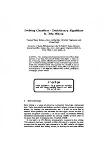
3.4.2. Information theoretic weighting of the values. Instead of using the weighting function Rv → [0, ∞[, r → qr np1 r we can consider the weigthing function r → − pr log( pr ) : for each variable (figure 1). Note, that using this weighting, as well the very likely events, i.e. values, which are shared by nearly all object, as very seldom events, i.e. values, which are shared only by a few objects, are weighted with a weight close to 0. The values, which occur with a probability in a medium range around p = 1e ≈ 0.36788 – the value, where the weighting function has its maximal value, also 1e , get the highest influence for the similarity. These considerations are justified by the concept of entropy from coding theory and information theory. It measures, which gain of information is received when one assigns an object to a cluster C. Let us assume that a given variable v has the discrete probability u} distribution ( p1 , . . . , ps ), if #Rv = s, in a given cluster with pu = #{x∈C|v(x)=r for 1 ≤ n u ≤ s and ru ∈ Rv . The entropy measure then is defined to be I ( p1 , . . . , ps ) = −

s

pu log pu ,

u=1

which motivates the above weighting concept. Note, that this measure can be derived from 4 axioms on basic requirements on such an entropy function, e.g. symmetry in all its variable number of arguments, continuity for the case of 2 outcomes, a norming condition and a recursive relation, see Renyi (1962). As before one can compensate by normalization.


Figure 1.

319

Entropy function x → x log(x).

Please see the following: In computer science usually one uses the logarithm with base 2, whereas in mathematics the so called natural logarithm is used with base e ≈ 2.71828. These logarithms with different bases are related as following: log2 x = log2 eloge x = (loge x)(log2 e) which means that the point where the extreme value of the weighting function occurs is the same. Therefore the choice of the base of the logarithm is more a question of convenience. 3.4.3. Arbitrary weights for pairs of values. In this section so far we have restricted the very general case of a similarity matrix—see 2.4.1—to the special case, where we basically compute the similarity by linear combinations of frequencies of at most 3 groups of values, namely = and = or =+ , =− , =. In the last two sections we universally attached weights individually to the pairs (r, r ) only. For situations, where one wants to have similarity influence of unequal pairs of values of a qualitative variable, too, a weight ωr,s should be provided for pairs of values.11 An obvious examples is to attach some similarity to the values red and orange for a qualitative variable colour. 3.5.

Mixed case

It remains the case of variables of mixed type. This means that the set of all variables consists of two disjoint subsets of variables, one which contains those of qualitative type, the other

320


one with all the variables of quantitative nature. Hence we have to combine the two similarity indices. The more general case is that we even distinguish different groups of variables of both types. Examples are different similarity indices for indicating and symmetric variables in the qualitative case or different similarity indices for various groups of variables. In cases, where all variables have to be considered simultaneously and with equal influence, it is convenient to scale the similarity index sG for the variables in a group G to range in [0, m G ], if a group G consists of m G variables. In the additive case we scale to [−m G , m G ]. A quantitative variable with range [0, smax ] and a threshold γ ∈ ]0, smax ] can be scaled by the linear transformation w →

1 γ w− smax − γ smax − γ

which is w → 2w − 1 in case of smax = 1 and γ = 12 to behave similarly to the additive case of qualitative variables, where the similarity value either is 1 or −1. Summing up all individual similarity indices for all groups G we receive an (additive) similarity measure, which ranges in [−m, m], with maximal similarity equal to m and maximal dissimilarity equal to −m. The case of unequal influence of the various groups of variables is easily by subsumed using the individual weights ωG . In this case the similarity range is [− G ωG , G ωG ]. 3.6.

Comparing an object with one cluster

Here we consider the (similarity) relations of a given object x ∈ O with a given cluster C ⊆ O. If we assume that a similarity index in normalized form s = ssma : O × O → [smin , smax ] as explained in Section 3.1 is given, then there is a natural extension of this index for qualitative variables. 3.6.1. Qualitative variables. To do so we consider the similarity function s : O × P(O) → [smin , smax ] y∈C sa (x, y) (x, C) → y∈C sm (x, y)

(3) (4)

where independently both for the actual and the maximal possible accordance the corresponding quantities of x compared to all the objects y in C are summed up. Note that these values lie in the same range [smin , smax ]. 3.6.2. Computational data structures and efficiency. During the process of deciding, whether the object x fits to cluster C it is crucial that the evaluation of s(x, C) respectively the comparison s(x, C) ≥ γ with a similarity threshold γ ∈ [smin , smax ] can be computed efficiently. The mere implementation of the summations of Eq. (4) requires 2 # C computations of the quantities sa (x, y) or sm (x, y) and 2 # C − 2 additions.


321

Let us compute sa (x, C) in case of sa (x, y) = a= (x, y):

sa (x, C) = sa (x, y) = a= (x, y) y∈C

=

y∈C

[v(x) = v(y)]

y∈C v∈V

=

(#{y ∈ C | v(y) = v(x)}) v∈V

Note that for sm (x, y) = a= + a= we immediately get sm (x, C) = m # C This suggests to code a cluster C by the distributions tC,v,r := (#{y ∈ C | v(y) = r })r ∈Rv of the values of all variables, which are stored in m tables tv , accessable by keys r in the range Rv . For such a data structure only m − 1 summations after m table accesses are required. The formula now writes

sa (x, C) = tC,v,v(x) . v∈V

Another simple computational improvement is gained from the fact that we do not really want to compute s(x, C) but only whether this value is larger than the given similarity threshold γ ∈ [smin , smax ], in case of [0, 1] often chosen to be 12 .12 The question whether s(x, y) =

sa (x, y) ≥γ sm (x, y)

is equivalent to sa (x, y) − γ sm (x, y) ≥ 0. In the important case of Jaccard and γ =

1 2

this is equivalent to

1 a= (x, y) − (a= (x, y) + a= (x, y)) ≥ 0 2 and hence to a= (x, y) − a= (x, y) ≥ 0. In this special case s could be defined to be s(x, y) := a= (x, y) − a= (x, y)

(5)

322


and its range are the integer numbers {−m, −(m − 1), . . . , −1, 0, 1, . . . , m − 1, m}. Here simply the number of matches is compared with the number of non-matches.13 The formula for s(x, C) in this important case then is s(x, C) = 2sa (x, C) − m # C with sa (x, C) =

tC,v,v(x)

v∈V

as

a= (x, y) =

tC,v,r =

v∈V r =v(x)

y∈C

#C − tC,v,v(x)

v∈V

= m # C − sa (x, C) Hence, the decision, whether x is similar to the cluster C, can be made according to either s(x, C) = 2sa (x, C) − m # C ≥ 0 or equivalently sa (x, C) ≥ m # C − sa (x, C). 3.6.3. Quantitative variables. We now assume that we consider continuous numeric v with range Rv = R asrandom variables with density φ : R → [0, ∞[, i.e. variables ∞ r ∞ φ(t) dt = 1 and P(v ≤ r ) = −∞ φ(t) dt, expectation value µ := −∞ tφ(t) dt, and −∞ ∞ 2 standard deviation σ := −∞ (µ − t) φ(t) dt, if these integrals exist. We assume further that a similarity index s : R×R → [smin , smax ] is given. In this setting it is natural to define the similarity of an outcome v(x) = r ∈ R w.r.t. v to be measured by s(r, v) :=

∞

s(r, t)φ(t) dt, −∞

provided the integral exists. This transforms directly to a cluster C, if we consider the restriction v|C of v to C and correspondingly φ|C , µ|C and σ |C : s : R × P(O) → [smin , smax ] ∞ (r, C) → s(r, t)φ|C (t) dt

(6) (7)

−∞

Note that this definition agrees with the summation in the case of qualitative variables by using the usual counting measure.


323

In the case that all quantitative variables are pairwise stochastically independent we can extend this definition to objects x ∈ O as follows: s : O × P(O) → [smin , smax ]

∞ (x, C) → sv (v(x), t)φv |C (t) dt v∈V

=

−∞

=

∞

∞

−∞

−∞

(8) (9)

sv (v(x), t) φv |C (t) dt

(10)

v∈V

s(x, t) φv |C (t) dt

(11)

where we have set s(x, t) := v∈V sv (v(x), t) and used the fact that the summation and the integal can be interchanged in the independent case. The case of dependent variables is not covered here, in this situation one has to consider the (joint) density of the random vector (v)v∈V . 3.6.4. Computational data structures and efficiency. In order to achieve reasonable assumptions on the distribution functions it is often advisable to cut off outliers by defining a minimal and a maximal value rmin and rmax . The fact that in general one does not have a-priori knowledge about the type of distribution increases the difficulties to get general implementations. Even under the assumption that a certain distribution is valid, one has to test and estimate its characteristic parameters as standard deviation σ and expectation value µ. Defining the standard deviation σ by setting 4σ = rmax − rmin could be one possibility. If furthermore the distribution has the expectation µ := rmin + 2σ = rmax − 2σ then by the inequality of Tschebyscheff an error probability of P(v < rmin ∧ v > rmax ) = P(| v − µ |≥ 2σ ) ≤ (2σ1 )2 σ 2 = 0.25 is left. If in a practical situation we have a normal distribution N (µ, σ 2 ) with its density φ(t) = 1 (t−µ) 2 1 − √ e 2 σ , then in this special case the error probability can be estimated to be less than σ 2π or equal to 0.05. One method to compute an approximation of the integral

∞

s(r, C) := −∞

s(r, t) φv |C (t) dt

for the value r := v(x) is to use a step function h instead of φv |C . In praxi this step function is determined by choosing values to be treated as outliers, i.e. the integral is restricted to [rmin , rmax ]. Then this interval is split in q subintervals – often called bucket—[rk−1 , rk ] of equal or distinct width wk := rk − rk−1 , where the value h k of h for the k-th bucket is defined to be the percentage h k :=

#{x ∈ C | rk−1 ≤ v(x) < rk } wk # C

324


of the objects in cluster C, whose values v(x) lie in the range [rk−1 , rk ], compare Section 2.1.3.14 Hence rk q

)2 − (t−r hk e dt rk−1

k=1

(t−r )2

can be used as an approximation for s(r, C) in the case of s(r, t) := e− . That means we are left with integrating t → s(r, t) over intervals. This is done in advance for all quantitative variables and stored for easy access during the computations. These precalculated values, depending on r , can be interpreted as weights for the influence of all buckets to the similarity of one value r compared to a given cluster C. As one possibility we mention that the Hastings formula can be used to approximate the exponential function by a low degree polynomial, see Hartung and Elpelt (1984) or Johnson and Kotz (1970).15 Note, that this implicit discretization of the continuous variable for these computational purposes, influences the similarity behaviour. 3.7.

Homogeneity within one cluster

3.7.1. Qualitative variables. Similarly as we have derived a similarity index s(x, C) for comparing an object x with a cluster C by using s(x, y) in the case of qualitative variables, we define an intra-cluster similarity h(C) to measure the homogeneity of the objects in the cluster. In case s(x, y) is defined as a ratio of actual similarity sa (x, y) and maximal possible similarity sm (x, y) we sum over all pairs of objects in the cluster individually for the numerator and the denominator: h : P(O) → [smin , smax ] C →

(12)

x,y∈C,x= y sa (x, y)

x,y∈C,x= y sm (x,

y)

.

(13)

Note that as before the range [smin , smax ] is not changed. In case the similarity index is given as a difference of desired matches and undesired matches—compare Section 3.6.2—we add up all similarities and divide by the number (#C 2) of pairs. h(C) =

1 #C 2

s(x, y)

(14)

x,y∈C,x= y

This could be interpreted as a mean similarity between all pairs of objects x ∈ y in the cluster C. Other measures of homogeneity can be found in the literature, e.g. h(C) =

min

x,y∈C,x= y

s(x, y).

A list of additional measures is given in Bock (1974, p. 91 ff.).

(15)


325

3.7.2. Quantitative variables. The methods of the last paragraph of the last section also apply to quantitative variables. Sometimes it is also convenient to drop the scaling factor, which gives as a measure for the homogeneity:

h(C) = s(x, y) (16) x,y∈C,x= y

3.7.3. Comparison with reference objects. An improvement on the computational complexity can be achieved, if a typical representative or reference object g(C) of a cluster is known. Note, that this even does not have to be an element of the cluster! Then instead of comparing all pairs of elements (of quadratic complexity) one only compares all elements of a cluster with its reference object:

h(C) = s(x, g(C)) (17) x∈C

In case of (at least) qualitative variables with values in a totally ordered range Rv one can use the median value m(v)—defined to be the value at position n2 if the cluster sample is ordered, i.e. the range of values v(x) for all x ∈ C (with repetition) is totally ordered—the median object g(C) := (m(v(x)))x∈C can be used. Another alternative is the modal value, i.e. the value of the range where the density has its maximum (we implicitly assume that the density under consideration is of unimodal type, i. e. has exactly one maximum). In case of symmetric densities this coincides with the expectation values. In case of quantitative variables with values in the normed vector space (Rm , · ), one can use as reference point the center of gravity of C, defined by g(C) :=

1 x. #C x∈C

The derived homogeneity measure

h(C) := x − g(C),

(18)

x∈C

is called within-class inertia and of cause should be a minimal as possible as it considers distances rather than similarities. 3.8.

Separability of clusters

3.8.1. Distances and similarities of clusters. As in Section 3.7 we can derive a distance measure for two clusters C and D, being disjoint subsets of the set O of objects s : P(O) × P(O) → [smin , smax ] (C, D) →

(19)

x∈C,y∈D sa (x, y)

x∈C,y∈D sm (x,

y)

(20)

326


in the case that s(x, y) is defined as a ratio of actual similarity sa (x, y) and maximal possible similarity sm (x, y). Note, that if it is guaranteed that for all pairs of objects x ∈ C and y ∈ D we have s(x, y) ≥ γ ∈ [smin , smax ] then we can conclude that the range of values of s(C, D) is [γ , smax ]. However, in the applications we are not so much interested in the similarity of two clusters, but in their dissimilarity, i.e. their separability. As we have to combine this with the intra-separability measure for each cluster, we have to use a distance function here and hence we define d : P(O) × P(O) → [smin , smax ] x∈C,y∈D (sm (x, y) − sa (x, y)) (C, D) → . x∈C,y∈D sm (x, y)

(21) (22)

Under this assumption the range of d actually is ]γ , smax ]. In the case of a similarity measure like s(x, y) = sa (x, y) − γ sm (x, y) we consider s(C, D) =

1

s(x, y) #C # D x∈C y∈D

(23)

This could be interpreted as a mean similarity between all pairs of objects x ∈ C and y ∈ D and is also called average linkage. Sometimes it is also convenient to drop the scaling factor, which gives

s(C, D) = s(x, y) (24) x∈C y∈D

Instead of using this average of all similarities, sometimes one works with the minimum or maximum only. The single linkage or nearest neighbourhood measure s(C, D) =

min s(x, y)

x∈C,y∈D

(25)

is often used in a hierarchical cluster procedure, see 5.2. If the similarity between their most remote pair of objects is used, i.e. s(C, D) = max s(x, y) x∈C,y∈D

(26)

then this is called complete linkage. In case all variables are numeric or embedded properly into a normed vector space (Rm , ·)16 , the center of gravity, or centroid g(C) :=

1 x #C x∈C

(27)


327

can be used to define a similarity measure s(C, D) = g(C) − g(D,

(28)

and is used in the centroid method. 4.

Criteria of optimality

As our goal is to find clusterings which both satisfies as much homogeneity within in each cluster as well as much separability between the clusters as possible, criteria have to model both conditions. It is then obvious, that criteria which only satisfy one condition usually have deficiencies like the cases in Section 4.1 will make clear. Therefore we shall present several criteria of optimality used to valuate a clustering and discuss the criterion in the following sections of this chapter. 4.1.

Criteria of optimality for intra-cluster homogeneity

One very popular criterion tries to maximize the similarities of the classes. This is described by the following optimization problem:

s(C) = s(C) → max (29) C∈C

C

where s(C) is a homogeneity measure, see Section 3.7. 4.1.1. The variance criterion for quantitative variables. Using the within-class inertia— see Eq. (18)—one gets the within-class inertia or variance criterion c(C) :=

1

x − g(C), n C∈C x∈C

(30)

which obviously has to be minimized and is best possible at 0. In case of all clusters being one-element subsets this is satisfied, we have optimal homogeneity for trivial reasons. In general we will have distributed similar objects into different clusters. Hence this criterion does not model our aims and is therefore only of minor help as criticized in Michaud (1995). Nevertheless, these kind of criteria can be useful in special cases. If the maximal number of clusters is given and is small, then the detected deficiency of this criterion obviously only plays a minor role. 4.1.2. Determinantal criterion for quantitative variables. This criterion is applicable for the case of m quantitative variables v ∈ V which we consider as one random vector (v)v∈V with expectation vector µ = (µv )v∈V . Furthermore it is assumed, that the—in general unknown—positive definite covariance matrix of this random vector is the same as for all its restrictions (v)v∈V|C to a cluster C of a clustering C.

328


It addition we also assume that the random vector is multivariate normal distributed by N (µ|C , C ) for each cluster C with expectation vector µ|C .17 In addition we assume for the whole section that also the object vectors x ∈ C are stochastically independent. We consider our setting of n objects O ∈ Rm as one random experiment in (Rm )n and—as we assumed the stochastic independence of the object vectors—with probability measure P being the direct product of the n copies of the object space. Hence, then the density of (v)v∈V on (Rm )n is the product of the densities on Rm . 4.1.2.1. Stochastically independent variables. Assume as introduction first that the covariance matrix C has a special structure, namely C = σ 2 Id, where Id is the unit matrix, i.e. the matrix with diagonal entries 1 and 0 elsewhere and σ the identical standard deviation of all variables v, i.e. all the involved m random variables are pairwise stochastically independent. If we assume that a clustering is already given with c clusters, then the density for all object vectors in one cluster C is determined by the parameters σ and µC by our assumption, hence φ(C, µ, σ ) =

1 (− 12 C∈C x∈C x−µC 2 ) 2σ . nm e 2 (2πσ ) 2

(31)

In practical situations usually the quantities µC for all C ∈ C and also σ are unknown and have to be estimated in order to find the clustering C. One very popular estimation method is the method of Maximum-Likelihood. Intuitively speaking it tries to find the most likely parameters determining a density, if the outcomes of the random vectors for each cluster are given. This can be achieved by maximization of the density on the product space, depending on the cm parameters µ|C v after inserting the mn measurements into Eq. (31). For practical purposes one usually first applies the monotonic transformation by log and receives the following symbolic solution for the estimators µ C =

1 x #C x∈C

σˆ 2 =

1

x − µ C 2 . nm C∈C x∈C

and

Here (under the above assumptions) µ C is obviously equal g(C), the center of gravity. Additionally, it can be shown that under relatively weak assumptions this method gives consistent and asymptotically efficient estimators of the unknown parameters, see e.g. Rao (1973, p. 353 ff. and ch. 6, p. 382 ff.). After inserting these estimators for the unknown parameters in the density we can then perform a second maximization step, this time with respect to all possible clusterings, as again maximizing the density improves the fitting of the parameters to the given data set. Hence, dropping the exponential functions and the constant positive factors, we directly


329

receive the variance criterion c(C) =

x − µ C 2 ,

(32)

C∈C x∈C

as in Eq. (18), which has to be maximized. Further details on this theorem can be found on Bock (1974, p. 115). An example, where this criterion works perfectly is represented in figure 2.

Figure 2.

Two independent populations, randomly generated around (0, 0) and (5, 5).

The two clusters representing these two populations both look like balls of constant radius. And this is the typical situation for the variance criterion which is best applicable in the case of variables, whose scale is of similar or equal magnitude. The plot was created by two bivariate normal distributions, whose expectation vectors were (0, 0) and (5, 5). The covariance matrix was equal

1 = 0

0 1

If one estimates the density, one gets the plot (figure 3):

330


Figure 3.

The density of two variables.

4.1.2.2. The general case. Now let us consider the general situation that all the object vectors of a cluster C are assumed to be multivariate normal distributed by N (µ|C , C ) for each cluster C with expectation vector µ|C and positive definite covariance matrix C = . As in the case of the variance criterion we have to consider the density for (Rm )n in this case, where no longer stochastical independence of the variables is true. φ(C, µ, σ ) =

1 (− 12 C∈C x∈C x−µC 2 −1 ) , n e (2π) (det ) 2 nm 2

√ where x −1 := x t −1 x is the norm, given by the Mahalanobis-distance, which is induced by the covariance matrix . This formula for the density can be rearranged and we get φ(C, µ, σ ) =

1 − 12 (tr(W −1 )+ C∈C #Cg(C)−µC 2 −1 ) n e (2π) (det ) 2 nm 2

by using centers of gravity and an inter-cluster covariance estimation W which is defined by W (C) =

WC (C)

C∈C

using the intra-cluster covariance estimations WC (C) =

(x − g(C))(x − g(C))t .

x∈C

As before we have to estimate the unknown expectation vectors µ|C and the covariance matrix . Using again the method of Maximum-Likelihood one gets the estimators µ| C =


331

ˆ we get g(C), the centers of gravity, and for W . n Inserting these estimators collapses the formula, after dropping constant factors and exponents we only keep ˆ =

φ(C) =

1 → min C det W

(33)

or equivalently c(C) = det W → max, C

(34)

which is called the determinantal criterion, for further details again see Bock (1974, in particular theorem 12.1 at p. 138). The figure 4 may give some deeper insight:

Figure 4.

Two populations, randomly generated around (0, 0) and (5, 5), but x- and y-variables dependent.

In this situation we have used the following covariance matrix : =

4 0.8 0.8 4

332


The obvious ellipsoidal structure of the two populations is due to the covariance matrix. It is obvious, that no cluster technique can separate these two populations perfectly, but the determinantal criterion is most appropriate as it favours this ellipsoidal structure. If one estimates the density in this case, one gets the plot (figure 5).

Figure 5.

The density of two clusters.

4.1.3. Trace criterion. Defining the quantity

B(C) = #C(g(C) − g(O))(g(C) − g(O))t C∈C

where we compare the centers of gravity of all the clusters with the overall center of gravity, allows to define the so called trace criterion:

c(C) = tr(W (C)−1 B(C)) = #C(g(C) − g(O))t W (C)−1 (g(C) − g(O)) → min . C

C∈C

where tr means the trace of a matrix. For additional information see Bock (1974, p. 191 ff.) or Steinhausen and Langer (1977, p. 105). Unfortunately, it is unknown until today under which assumptions this criterion should be recommended. 4.2.

Criteria of optimality for inter-cluster separability

Similar as in the case for intra-homogeneity we get criteria for optimizing the inter-cluster separability of a clustering by adding up all distances d(C, D) between two different clusters C and D.

d(C) = d(C, D) → max (35) C,D∈C,C= D

C

where d(C, D) is a separability measure, see Section 3.8.

333


4.3.

Criteria of optimality for both intra-cluster homogeneity and inter-cluster separability

It is clear by now, that the definition for criteria which satisfy both requirements of intracluster homogeneity and inter-cluster separability has to be as follows: 



  c(C) =  h(C) + d(C, D) → max C∈C

(36)

C

C, D∈C C=D

where h(C) is a homogeneity measure and d(C, D) is a separability measure. In the case of having as building blocks a similarity index s : O × O → [smin , smax ] and a corresponding distance function d : O × O → [smin , smax ] we can again discuss the two major situations. First, if the functions are normed, i.e. given as a ratio of sa and sm and have their range in [0, 1], second if this is not the case. 4.3.1. Criteria based on normed indices. In the first case use s = define

sa sm

and d =

sm −sa sm

and

c : {C ⊆ P(O) | C is a clustering of O} → [0, 1] by setting

C∈C

c(C) :=

x,y∈C,x= y sa (x,

y)

C∈C

x∈C,y∈O\C (sm (x,

x,y∈O,x= y sm (x,

y) − sa (x, y))

y)

For a given threshold γ ∈ [0, 1] we can compute equivalent conditions for c(C) ≥ γ . c(C) ≥ γ

sa (x, y) +

C∈C x, y∈C x=y

C∈C

≥γ

sm (x, y)

x,y∈O,x= y

+

C∈C

x∈C y∈C\C

(sm (x, y) − sa (x, y))

x∈C y∈C\C

(sa (x, y) − γ sm (x, y))

C∈C x, y∈C x=y

((1 − γ )sm (x, y) − sa (x, y)) ≥ 0

334


In case of symmetric variables with sa = a= and sm = a= + βa= , see Section 3.2.1, the last conditions rewrite to

(a= (x, y) − γ (a= (x, y) + βa= (x, y)))

C∈C x, y∈C x=y

+

C∈C

((1 − γ )(a= (x, y) + βa= (x, y)) − a= (x, y)) ≥ 0

x∈C y∈C \ C

((1 − γ )a= (x, y) − γβa= (x, y))

C∈C x, y∈C x=y

+

C∈C

Setting γ := summand

1 2

((1 − γ )βa= (x, y) − γ a= (x, y)) ≥ 0

x∈C y∈C\C

and multiplication of the whole expression by 2 yields the (intra cluster)

(a= (x, y) − βa= (x, y)) and the (inter cluster) summand (βa= (x, y) − a= (x, y)). 4.3.2. Criteria based on additive indices. In the second case we use d = −s and set c(C) =

C∈C x,y∈C,x= y

s(x, y) +

d(x, y)

(37)

C∈C x∈C y∈O\C

which simplifies in case of d = −s to c(C) =

(−1)[∃C∈C|x,y∈C] s(x, y)

(38)

C∈C,x= y

As usual one can scale the value by dividing by the number of pairs (n2). 4.3.3. Updating the criterion value. In continuation of Section 3.6.2 we discuss efficient data structures for updating the criterion value in this important case. We shall see in Section 5.3.1 how to initially build a clustering by successive construction of the clusters considering a new object x and assign it to one of the already built clusters or create a new cluster. Alternatively, one tries to improve the quality of a given clustering by removing an element x from one of the clusters and reassign it. In both cases the task of computing c(C # ) from c(C), if C # is constructed from C = {C1 , . . . , Ct } by assigning x either to one Ca or to create Ct+1 := {x}.


335

Let us assume that each cluster C ∈ C is given by a vector of tables, where each table t corresponds to a variable v ∈ V and contains the value distribution of this variable in the cluster C. The tables are key-accessable by the finite values of the range Rv in the case of qualitative variables. In the case of quantitative variables, it is assumed that we have defined a finite number of appropriate buckets, which are used to count the frequencies and to access the table. With this data type it is very easy to compute

a= (x, C) = tC,v,v(x) v∈V

where tC,v,v(x) := #{y ∈ C | v(y) = v(x)}. This requires m table accesses and additions. We immediately get also a= (x, C) = m # C − a= . If we further assume that s(x, y) = a= (x, y) − a= (x, y) and d(x, y) = −s(x, y) = a= (x, y) − a= (x, y) then we can update

c(C) = h(C) + C∈C

d(C, D)

C,D∈C,C= D

where h(C) is from (16) and d(C, D) from (24) by means of h(C ∪ {x}) = h(C) + s(x, C) and d(C ∪ {x}, D) = d(C, D) + d(x, D). Hence we build the sum

u(x) := d(x, C), C∈C

which is the update for the case Ct+1 = {x}. The update for the other c possibilities can be computed by the formula u(x) − d(x, C) + s(x, C).

336


During the computations it is also possible to compare for the maximal update, which gives the final decision, where to put x. Note also, that s(x, C) + d(x, C) = m#C. The complexity of this update and decision procedure for one of the n elements x is linear in m and c. 4.3.4. Condorcet’s criterion: Ranking of candidates and data analysis. In 1982 J.-F. Marcotorchino and P. Michaud have related Condorcet’s solution of 1785 to the ranking problem with data analysis—see the series of technical reports (Michaud, 1982, 1985, 1987a). The theory around this connection is called Relational Data Analysis, for historical remarks see Michaud (1987b). Suppose there are n candidates x (i) for a political position and m voters vk , who rank the candidates in the order of their individual preference. This rank is coded by a permutation πk of the symmetric group Sn , i.e. voter vk prefers candidate x (πk (i)) to x (πk ( j)) for all 1 ≤ i < j ≤ n, i.e. the i-th ranked candidate is x (πk (i)) . To solve the problem of the overall ranking, i.e. the ranking, which fits most of the individual rankings, Condorcet has suggested to use a paired majority rule to choose λ ∈ Sn , which determines the overall ranking x (λ(1)) < x (λ(2)) < · · · in such a way that the number of votes

# k | πk−1 (λ(i)) < πk−1 (λ( j)) 1≤i< j≤n

—which places candidate x (λ(i)) before x (λ( j)) , for all (n2) pairs (λ(i), λ( j))—is maximized. Note, that he suggested to dissolve the question of ranking n candidates to the more general task to answer (n2) questions: Do you prefer candidate x (i) to x ( j) ? Hence it is clear that the majority of votes #{k | πk−1 (i) < πk−1 ( j)} ≥ m2 for ranking x (i) before x ( j) and not x ( j) before x (i) , in general only determines a relation on the set of candidates. There is no necessity to get unique solutions for the ranking, as it can be very well the case that there is a majority of votes for ranking x (i) before x ( j) , x ( j) before x (k) , but also x (k) before x (i) —a phenomenon which is called Condorcet’s effect to avoid the misleading term paradox. Now instead of ranking candidates, the variables v are considered as voters, which vote for or against the similarity of the objects x and y. To make this more precise, the values v(x) and v(y) are compared and used to decide the question, whether x and y are considered to be similar [v(x) ∼ v(y)] or dissimilar [v(x) ∼ v(y)], i.e. whether the variable v votes for putting both objects into one cluster or into two different clusters. As appropriate the vote can be measured by equality in case of binary or arbitrary qualitative variables or by lying within a given distance—see 3.3—for quantitative variables. As before we count all votes for a given clustering C. Again we use the Kronecker-Iverson symbol, see Section 2.4.1.

c(C) = [v(x) ∼ v(y)] + [v(x) ∼ v(y)] (39) C∈C x, y∈C v∈V x=y

C∈C

x∈C v∈V y∈O\C


=

s(x, y) +

C∈C x, y∈C x=y

=

C∈C

h(C) +

d(x, y)

337 (40)

x∈C y∈O\C

d(C, D)

(41)

C,D∈C,C= D

C∈C

where we used the homogeneity function

h(C) :=

a= (x, y)

x,y∈C,x= y

based on the similarity index s(x, y) =

[v(x) ∼ v(y)] v∈V

and the distance function

d(C, D) :=

a= (x, y)

x∈C,y∈D

based on the distance index d(x, y) =

[v(x) ∼ v(y)] = a= (x, y) = m − a= (x, y). v∈V

Now in principle it is possible to find the best possible clustering, the one, which gets most votes. This criterion is called Condorcet’s criterion. Subtraction of m2 (n2) and the use of a= (x, y)+a= (x, y) = m transfers this voting criterion to c(C) =

m m a= (x, y) − + − a= (x, y) 2 2 C∈C x, y∈C C∈C x∈C x=y

(42)

y∈O\C

Multiplication by 2 results in c(C) =

C∈C x, y∈C x=y

(a= (x, y) − a= (x, y)) +

C∈C

(a= (x, y) − a= (x, y))

(43)

x∈C y∈O\C

and this can be interpreted by setting a new similiarity index to s(x, y) := a= (x, y) − a= (x, y) and a new distance index to d(x, y) := a= (x, y) − a= (x, y) with range [−m, m] as in formula (5). We illustrate this in the Appendix A by an example.

338


4.3.5. The C∗ -criterion. This criterion, which was derived from Condorcet’s work is closely related to the C ∗ -criterion,—see e.g. Bock (1974, p. 205 ff.)—which had already been suggested in Fortier and Solomon (1966). It can be interpreted as follows by accepting a similarity threshold value γ , originally denoted by c∗ . For the partition C to be found – the pairs of objects x and y with s(x, y) ≥ γ —which means similar objects—should be members of the same cluster and contribute their strength of similarity given by s(x, y) − γ , while – pairs of objects with s(x, y) < γ should be contained in different clusters of C and contribute their distance given by γ − s(x, y). This means that a clustering C is the better, the larger the expression

(s(x, y) − γ ) + (γ − s(x, y)) C∈C x, y∈C x=y

C, D∈C x∈C,y∈D C=D

is, compare (42). This optimization criterion can be rewritten as

c(C) = (−1)[∃C∈C|x,y∈C] (s(x, y) − γ ). x,y∈O,x= y

Relaxing from accepting the threshold γ = m2 to using the derived similarity index [s(x, y) ≥ γ ] and after choosing the new γ := 12 , this criterion rewrites to

C∈C x, y∈C x=y

1 [s(x, y) ≥ γ ] − 2

+

C, D∈C C=D

1 − [s(x, y) ≥ γ ] , 2 x∈C,y∈D

which is equal to (1) for x ∼ y :⇔ s(x, y) ≥ γ . 4.3.6. Other criteria. There are other criteria definitions proposed in the literature, which are beyond the scope of this paper. One example is the following ratio of the sum of homogeneities s(C) of a fixed number of clusters and the sum of the inter-cluster similarities s(C, D): s(C) c(C) = C∈C → max . C s(C, D) C= D This criterion does make sense in particularly, if an average similarity is used to guarantee values in [0, 1], see e.g. Bock (1974, p. 204). 5.

Construction of clusterings

In this chapter we give a classification of a large variety of clustering algorithms and visualize it by a tree-like graph. The graph is not symmetric, as we focussed on the best


339

known algorithms from the literature. The various algorithms are given in a quite generic form. Traditionally there are two different classes of algorithms to solve the clustering problem. In Section 5.2 we will discuss hierarchical clustering algorithms. Here one does not get a single clustering as the final result, but a sequence of clusterings, which are refined successively. In Section 5.3 so called partitioning cluster algorithms will be discussed. Some of these algorithms require that the maximal number c of classes is defined in advance. In Section 5.4 we discuss neural network simulation methods for finding clusterings. 5.1.

A tree-like guide to clustering algorithms

We have constructed a tree (figure 6), which tries to classify the most important clustering algorithms according the line of this paper, see the following graphic. The first classification point is the one where one separates hierarchical methods (which work with refinements of clusterings, we will explain that a little bit later) and partitionings in the sense that either one tries to find a optimal clustering for a desired or predetermined number of clusters or one tries to find an as good as possible clustering where the number of clusters is not known in advance. Hierarchical methods can be divided into additional classes, we will explain that later on. Partitioning algorithms can be classified additionally by the variables they use (quantitative or qualitative) and of course by the mechanisms how the clusters are built. 5.2.

Hierarchical methods

There are two different methods to construct a hierarchy. One distinguishes between a bottom-up approach and a top-down approach. The bottom-up approach starts from the finest clustering consisting of n 1-element clusters given n objects and finishes at the most coarse clustering with one cluster consisting of all n objects. Methods, which generate a hierarchy in such a way, are called agglomerative methods and discussed in Section 5.2.1. The top-down approach works in the other way from the most coarse partition to the finest partition. The methods using this approach are called divisive methods and discussed in Section 5.2.3. In both cases the graphical representation of the results often is done by trees called dendrograms, see Section 6.3. A hierarchy H is a system of subsets of the object set O = {x (1) , . . . , x (n) }, where all sets of H are different, their union is O and where for every two sets C, D ∈ H, C = D only one of the following three alternatives is possible – C∩D=∅ – C⊂D – D ⊂ C, see also Bock (1974, p. 360). The most typical case is that we have n levels of sets, in level h i there are exactly i subsets constituting a clustering of O. The transition from level h i to

340

Figure 6.


Classification of clustering techniques.


341

level h i−1 is determined by splitting exactly one set of level h i into two non-empty subsets for level i − 1. All other sets remain unchanged. Here we have a simple example for such a situation: h6 h5 h4 h3 h2 h1 h0

{1, 2, 3, 4, 5, 6, 7} {1, 2, 3, 4, 5}{6, 7} {1, 2, 3, 4, 5}{6}{7} {1, 2, 3}{4, 5}{6}{7} {1, 2}{3}{4, 5}{6}{7} {1}{2}{3}{4, 5}{6}{7} {1}{2}{3}{4}{5}{6}{7}

This gives rise to define the following notion: A hierarchy of clusterings is a sequence of l(≤ n) partitions C 1 , . . . , C n , where C (i+1 ) is a refined clustering of the clustering C (i) for all 1 ≤ i < n. The number (n) of all hierarchies n−1 nof clusterings of a set O with n elements can be determined recursively by (n) = i=1 { i }(i). Typical situations, where the interest lies in the whole hierarchy arise from zoology and botany, where one is not only interested in the clustering given at by the leaves, but each level of the hierarchy corresponds to a named family as mammals or vertrebrates of animals or plants. If the number of clusters is given, then one can stop at the corresponding level. In case this is not given, we are also faced with the problem of cutting the tree at some level to get a clustering. The considerations in Section 4.1.1 imply that in general it will not be clear, what is the best one. 5.2.1. Agglomerative methods. The fundamental steps of any agglomerative method are as following: Algorithm – A population O, – a distance function d : P(O) × P(O) → [dmin , dmax ]. step 1. Start with the finest clustering

INPUT:

h 0 := {{x} | x ∈ O}, i.e. the partition, which consist of n one-element clusters. step 2. Find the two clusters C and D with the smallest distance d(C, D) among all pairs of clusters. step 3. Combine this two clusters C and D to one new clusters, hence reducing the number of clusters by 1 and receiving the clustering h i from h i−1 . step 4. Stop after n − 1 steps, i.e. when we are left with one single cluster consisting of all elements. OUTPUT: Return the hierarchy (h 0 , h 1 , . . . , h n−1 ) of clustering of O.

342


The remaining freedom in this procedure is the choice of a distance function d : P(O) × P(O) → [dmin , dmax ]

(44)

as discussed in Section 3.8. The hierarchical cluster algorithms are mainly named after this choice of distance function. There is an enormous variety of methods in the literature. The books (Bock, 1974, p. 387 ff.; Steinhausen and Langer, 1977, p. 76 ff.) list about a dozen methods. We will comment the typical behaviour of some of the methods, due to the fact that the methods differ all in the way they fuse two clusters to a larger cluster and hence behave in a different manner . – The single-linkage method or nearest neighbour method, for the similarity function see (25). This method has a strong tendency to chaining in a geometrical sense and not balls, an effect, which is not desired in some applications; groups, which are not separated quite well cannot be detected, see Steinhausen and Langer (1977, p. 78). – The complete-linkage method with similarity function (26) has the tendency to build small clusters , see Steinhausen and Langer (1977, p. 78). – The average-linkage method builds some compromise between the two extreme cases of single-linkage and complete-linkage. Usually it leads to quite reasonable results. Its similarity index is (23). – The centroid method preassumes the Euclidean norm and behaves as following: Those groups are combined, whose centers of gravity have the smallest distance, see (28). In case of arbitrary distance functions it cannot be recommended due to the point that it leads to results which are difficult to interpret, see Steinhausen and Langer (1977, p. 79). – The weighted average-linkage method is slightly more general than the centroid method. Usually, it leads to good results, too. – The median method should be used with care, see Steinhausen and Langer (1977, p. 79). In this book several difficulties related with this method are explained in larger detail. – The method of Ward is similar to the centroid method, but contrary to the centroid method the most similar groups are combined, see Bock (1974, p. 407 ff). It has the advantage that also in case of other distance functions than the Euclidean one it leads to reasonable results, see Steinhausen and Langer (1977, p. 81). The only distinction of these methods is according to their distance functions d(C, D) to decide the question whether C and D are fused. 5.2.2. Computational efficiency. The various agglomerative methods use different distance functions on the power set P(O) as explained in Section 3.8. For computational efficiency at each level of the hierarchies, one does not want to compute the distances d(C ∪ D, E) of the recently fused cluster C ∪ D and all the other fixed clusters E ∈ C from scratch. In most cases this can be done recursively by building linear combinations of d(C, E), d(D, E), d(C, D) and |d(C, E) − d(D, E)|. In Bock (1974, p. 404) a complete table of all the mentioned methods can be found.


343

5.2.3. Divisive methods. Contrary to the agglomerative methods such procedures start with the largest clusterings, i.e. the clusterings with exactly one cluster. This cluster will be separated into two clusters in the sense that one tries to optimize a given optimization criterion c. After the separation into two clusters the clusters itselves are split into two clusters until a separation into two clusters correspondingly is no longer possible. Essentially there are two alternatives to split the classes: – Polythetic methods, which use all variables for the successive splits. Here we refer to the methods by Edwards/Cavalli-Sforza and Gower in the case of quantitative variables—see Bock (1974, p. 412 ff.)—and in the case of qualitative variables the method by Orloci, see Bock (1974, p. 414). – Monothetic methods, which use only one variable for the successive splits. One popular representative is the method by Lance/Williams, described on Bock (1974, p. 417 ff.). Compared with the agglomerative methods usually the divisive methods need much more computing power, see Steinhausen and Langer (1977, p. 100). Unfortunately the received results are usually worse than in the case of agglomerative methods. Therefore it suffices to mention the existence of such methods, but not going into details. 5.3.

Partitioning algorithms

From the complexity of the problem to find a best clustering or at least very good clusterings for a given set O of n objects, it should be clear, that a hierarchical method can only be feasible in very specific cases. But such a method could be used for an initial clustering. More important are the so-called partitioning algorithms where contrary to the hierarchical methods each object will be attached individually to a cluster. Hence, once we got an initial clustering we can modify it properly to recursively receive better iterations, perhaps even allowing clusterings, where the criterion decreases its value on intermediate iterations. 5.3.1. Construction of an initial clustering. Certainly one can use a hierarchical method to get an initial clustering. Also a random clustering can be used as start clustering. In the sequel we give and discuss various techniques. If there are further constraints given as the maximal number of clusters or minimal size of a cluster, these methods easily can be adjusted accordingly. 5.3.2. Initial clustering: Most general case. In the most general case one can proceed as follows. Algorithm – A population O, – a criterion c : {C clustering} → [smin , smax ]. step 1. Set C := ∅. step 2. Iterate over all elements x in O:

INPUT:

344


step 2.1. Iterate over all t already constructed clusters C ∈ C, recalculate c(C) under the assumption that x is put in C. step 2.2. Consider to build a new cluster {x}, consisting of x exclusively and potentially put the one element cluster {x} into C and recalculate c(C) too. step 2.3. Among the t + 1 possibilities choose the clustering, which gains the highest value of c(C). OUTPUT: Return the clustering C. The algorithm requires in particular an efficient update of c(C), see Section 4.3.3! This has to be done in at most n(t + 1) cases, if c is the number of clusters and n the number of objects. Note, that in this general setting as well as in the following two modifications of it the initial clustering depends on the ordering of the elements. Several iterations of the algorithms as discussed in Section 5.3.7 will decrease this dependency. This is basically the algorithm implemented with Condorcet’s criterion in IBM’s Intelligent Miner and called demographic algorithm18 and the whole methodology also was called relational data analysis (RDA) to refer to the connections between Condorcet’s criterion—see Section 4.3.4—and related equivalence relations—see Sections 2.4.1. Note, that the demographic algorithm is iterative and repeats the steps of the initial clustering according to Section 5.3.7 a user defined number of times. Overall it is linear in the number of objects, the number of variables, the number of clusters and the maximal number of values/buckets of the quantitative variables. Note, that the summation over all values/buckets only occurs during the computation of the similarity integrals for quantitative variables. 5.3.3. Initial clustering: Intra-cluster homogeneity. If the criterion c(C) = C∈C h(C) is only based on the intra-cluster homogeneity of the clusters as discussed in Section 4.1, then the following method is possible. Note, that we select the cluster according to the nearest neighbourhood. Algorithm – A population O, – a homogeneity index h : P(O) → [0, 1], – and a similarity threshold γ ∈ [smin , smax ]. step 1. Set C := ∅. step 2. Iterate over all elements x in O: step 2.1. Iterate over all clusters C ∈ C, consider putting x in C and update h(C) under this potential modification. step 2.2. If there is a cluster C, where the updated h(C) ≥ γ , we finally put x in that cluster C, where h(C) is maximal, step 2.3. else form a new cluster {x} and put it into C OUTPUT: Return the clustering C. INPUT:


345

For the latter algorithm it is assumed implicitely, that we have normed the homogeneity values. In case of additive measures appropriate modifications have to be made. The threshold value γ is essential and can be used to steer the number of clusters. Usually the number of formed clusters decreases with the decrease of the threshold γ for the similarity. The method of Dorofeyuk drops threshold γ , but fixes in advance the number c of clusters instead. To start with the algorithm takes the first c elements and builds c oneelement clusters. Then it iterates through the other elements as in this algorithm by taking the maximal values of s(x, C). He does not restrict himself to quantitative variables, but allows arbitrary variables and similarity functions, see Bock (1974, p. 297). 5.3.4. Initial clustering: Nearest-neighbourhood-type algorithms. If one rewrites this algorithm focussing only on the updates of the homogeneity measure, we quite naturally receive the method, which is used in nearest-neighbourhood-algorithms and was proposed originally by Lu and Fu in 1978, see Jain and Dubes (1988, p. 28). Note also, that the algorithm can be implemented by using a distance index d(x, C) instead of a similarity index s(x, C). Originally, the maximal distance was used, but from our setting it is clear that any distance measure can be used. Algorithm – A population O, – a function s : O × P(O) → R, – and a similarity threshold γ ∈ R. step 1. Set C := ∅. step 2. Iterate over all elements x in O: step 2.1. Iterate over all clusters C ∈ C until s(x, C) ≥ γ . step 2.2. If such C’s are found, finally put x in that cluster C, where s(x, C) is maximal, step 2.3. else form a new cluster {x} and put it in C step 3. Return C. OUTPUT: Return the clustering C. INPUT:

Often in praxi one is content by taking the first cluster C, where s(x, C) ≥ γ . Obviously, these algorithms require at most n(c + 1) steps, if n = #O and c = #C. In the first case there are at most n(c + 1) updates and comparisons of the h(C)’s, in the second case the same number of computations of s(x, C). 5.3.5. Initial clustering: Clusters around kernels of typical elements. The next idea to create an initial clustering is always to use a typical element as the kernel of a new cluster, which is then enriched until a threshold is reached. Hence the method requires a function g : P(O) → O, which determines a most typical or representative element of a set. The algorithm does not directly use a criterion, but only the constituents h and s. It requires n (n + 1) computations of s(x, C), but in general it is robust against permutations of the 2 objects. This method for gaining an initial clustering is proposed at in Bock (1974, p. 225 ff.).

346


Algorithm – A population O, – a function g : P(O) → O, – a function h : P(O) → [smin , smax ], – a function s : O × P(O) → [smin , smax ], – and a similarity threshold γ ∈ [smin , smax ]. step 1. Set U := O and C := ∅. step 2. Take the most typical element x := g(U) of U and consider this to be the kernel of the next cluster, i.e. C := {x} and update C to be C ∪ C. step 3. Set U := O \ {x} and find an element y in this set of objects, not yet classified, which has the largest similarity s(y, C) compared to C, add y to C and remove it from U. step 4. Repeat step 3 until the homogeneity h(C) of the cluster C is smaller than the given threshold γ . step 5. Now separate C from O and repeat steps 2 and 3 to get the next cluster. Similar iterations until U is consumed result in a sequence of disjoint clusters Ca , hence a clustering C := {C1 , C2 , C3 , . . .}. OUTPUT: Return the clustering C. INPUT:

Examples for the function g are e.g. the center of gravity, the vector of medians or simply a random element, certainly of different behaviour! Another method is to look how many elements of the population are in a γ —neighbourhood of the elements and to choose the element with the maximal number of neighbours. A variation of this method is to simultaneously start with a number c# of typical elements, which will change during the algorithm. This was first suggested by G.H. Ball and D.J. Hall in a series of papers between 1965 to 1967 or Bock (1974, p. 233 ff.). Their implementation of the algorithm was called ISODATA. They have imposed additional contraints by homogeneity and distance thresholds by using the cluster distance given by the centers of gravity, which can also have the effect that the clustering is non-exhaustive, i.e. some elements can not be sorted in the actual clusters and are also forbidden to form clusters of their own. To put this into our framework one could relax these constraints in these cases. Further information about ISODATA can be found in the books (Bock, 1974, p. 233 ff.); Kaufman and Rousseeuw, 1990, p. 115 ff.; Jain and Dubes 1988, p. 98 ff.; Seber, 1984, p. 380 ff.). In Bock (1974, p. 234) there are some remarks with respect to the efficiency and quality of ISODATA. It is pointed out that in the case that the variables restricted to the individual clusters are multivariate normal distributed with the same covariance matrix, ISODATA gives quite acceptable results, whereas in case of different covariance matrices the results became worse. For their improvement process see Section 5.3.7. 5.3.6. Initial clustering: Clusters around moving kernels of typical elements. In addition to the methods of Section 5.3.5, where a typical element, which builds the kernel of a cluster, remains fixed under the whole process and only can be changed at further improvement steps as described in Section 5.3.7, the typical elements are subject to changes each time an element x is considered. This can be modelled by allowing x to be a second argument for the function g.


347

Again the algorithm does not directly use a criterion, but only the constituents s, respectively a corresponding distance index d. Hence, only a criterion, which optimizes the cluster homogeneity, can be represented. Contrary to above we formulated the variation where the algorithm directly starts with c# kernels. Furthermore, not the best fitting element is searched, but simply the next one is taken. Algorithm – A population O, contained in a set U, – a function g : U × O → U, – a function d : U × U → [smin , smax ]. # step 1. Choose c# most typical elements (prototypes) {y (1) , . . . , y (c ) } ∈ U as prototypes of the cluster, i.e. Ca := {y (a) } for all 1 ≤ a ≤ c# and # C := {{y (1) }, . . . , {y (c ) }} step 2. Iterate over all elements x ∈ O: step 2.1. Compute d(x, y) for every cluster C ∈ C with typical element y and compare the values. step 2.2. Put x in C where d(x, y) is minimal for corresponding prototype y. step 2.3. Update all prototypes, i.e. ya# := g(ya , x). OUTPUT: Return the clustering C. INPUT:

Note, that we formulated the algorithm in such way, that it is not necessary, that the kernels are elements of the population set O, but could be member of a larger universum U ⊇ O. This makes sense in particular in the case of quantitative variables exclusively, where the kernels can have a geometrical meaning. It should be clear as well that instead of measuring the distances d(x, C), one could also compute a given criterion c(C # ) for all cases of putting x into one of the c# clusters to get C # and then let the cluster win, where the best improvement for the criterion is achieved. 5.3.6.1. K-means clustering for quantitative variables. Using the distance d(x, C) := x − g(C) of x to the center of gravity g(C) in the above algorithm gives the popular K -means algorithm.19 It minimizes the within-class-inertia criterion, see Section 4.1.1 and does not focus on separability. 5.3.6.2. The case of normed quantitative variables. The case of quantitative variables x with normed values in [0, 1] is of particular interest. Let w be the most typical element for a cluster C. Then we can use as distance index d(x, C) := d(x, w) := x − w. In case of the Euclidean norm finding the minimal value of expressions like m d(x, w) := x − w = (x j − w j )2 k=1

m m m

= x 2j − 2 xjwj + w 2j k=1

k=1

k=1

348


it is equivalent to find the maximal value of the scalar products s(x, C) := xw t =

m

xjwj

k=1

for w ∈ C. Depending on a scaling factor η ∈ [0, 1] we can set g(x, w) :=

w + η(x − w) w + η(x − w)

(45)

to move the old winning kernel w according to the factor η into the direction of x. The other centers are not changed. As the typical elements are changed during the steps of the algorithms, it is quite natural to ask for conditions, under which this process converges. A question is, whether, e.g. w converges against the center of gravity of its cluster? The second question is, under which conditions does this clustering process converge against a good clustering in the sense of an optimization criterion to be defined for this approach. This kind of problems is studied since the fifties within the theory of stochastic approximation methods, see e.g. Robbins and Monro (1951). As explained before in Section 2.3 we consider the iteration process through all the objects x ∈ O as n repetitions of a statistical experiment, i.e. as a stochastic process x(i) depending on a discrete time 1 ≤ i. Hence it also can be assumed that the scaling factor η is time-dependent, for simplification we write η(i). The result of Robbins and Monro is as follows. For notational simplification let us assume that during the whole process always a particular cluster C is winning. If the sequence η(i)i∈N satisfies the conditions ∞

η(i) = ∞

i=1

and ∞

η(i)2 < ∞

i=1

then the sequence recursively defined by (45) with arbitrary w(0) and w(i + 1) := w # , w(i) := w, converges at the center of gravity of the cluster C. There are some further technical conditions to be fulfilled, see Robbins and Monro (1951). These conditions are necessary to force a certain stabilization, which is due to the second condition on one hand and on the other one to prevent that the process dies out, which is the first of the above conditions. The conditions for the general case—namely that each subsequences defined by each cluster converges to the center of gravity of the cluster can easily be derived. In 1966 Braverman in a special case and in 1967 in a much more general setting Tsypkin and Kelmans applied the approach by Robbins and Monroe to the clustering problem. The theoretical lines of the algorithm by Tsypkin/Kelmans and the essential proofs for the convergence against the true centers can be found in the book by Bock (1974, p. 279 ff., ch. 29).


349

5.3.7. Improvements of clusterings. Once a first clustering is given or found, there are several possibilites for improvements. One natural way to improve is to perform a number of iterations, each time working through the whole population. This makes sense especially for the methods described in the Sections 5.3.2 and 5.3.3. Each large improvement step iterates over all elements x of the population and removes it from its cluster, where it was located in the previous large step. Then it is considered as a newly given element, where the location within one of the actual clusters or as the first element in a new cluster, has to be found. This means, that instead of building a clustering from scratch, this time we use the actual clustering and modify it accordingly. It does not make immediate sense to iterate again through the objects if one works with typical elements as in Section 5.3.5. Here first other strategies to fuse or to split cluster have to be employed. If the homogeneity of a cluster is or becomes smaller than a given threshold γ , then the cluster is split in parts. If the distance between two clusters is or becomes smaller than a given threshold δ, then the two clusters are fused. After this partial step the number of clusters or the clusters itselves are changed, hence there are new typical elements. These can be used to repeat the construction as described in Section 5.3.5. Alternatively, it is possible to modify the algorithms in the spirit of simulated annealing methods, where one does not always use the locally best improvement, but has a random generator, which chooses the way to proceed. This allows in particular to decrease the criterion value and opens up the possibility to escape from local maxima. 5.4.

Neural network simulations

During the last years there were some remarkable developments in the area of neural networks related to clustering problems. Here it is assumed that all the m variables are quantitative, the object universe being Rm . Often it is recommended that the values of the variables all are standardized (normed) to range in [0, 1], which keeps them comparable— see also Section 2.4.1. Simulation of neuronal networks is done by modelling processes in the human brain, where input signals are transferred by axones via chemical connections, the so called synapses into the neurons, which send out new output signals, if they get enough input activation. Hence these neurons build transition elements and are connected to form a neural network, sometimes structured by various layers. 5.4.1. Neural network clustering with unsupervised learning. The number c of clusters is assumed to be given. In the easiest case of only one input layer and one output layer, we construct one output neuron for each cluster. Each of the m variables corresponds to exactly one input neuron. The network consists of all m × c connections and can be depicted by the following directed graph, here for m = 4 and c = 3. The figure 7 only shows the edges to cluster 1 and cluster 3. The output neurons are modelled also by elements w ∈ Rm respectively [0, 1]m . In the simulation model the connecting edge of input of variable i is labelled with wi and hence called synapse weight. The input objects x ∈ O to be clustered are considered as input signals xi for the input neuron i. The joint signal for output neuron modelled by w is then

350


age

x1

w 1 (1) w1

income

(3)

w3 w2

gender

cluster 1

w 2 (1)

x2

(1)

w 4 (1)

(3)

cluster 2

x3 cluster 3 winning !

w 3 (3) car

x4

w 4 (3)

input layer

Figure 7.

weights

output layer

Neural net.

defined to be the scalar product xw t = m k=1 x k wk of x and w. According to the strategy called the winner takes it all the output neuron resp. the corresponding cluster, which gets the highest (largest) signal xwt wins and the object x is put into this cluster. We did not yet define the various weights w. They are chosen randomly at the beginning and are updated after each assignment step. This is the so-called unsupervised learning of the neural network. It is typically implemented by w# :=

w + η(x − w) w + η(x − w)

which moves the old weight element w into the direction of x with an amount of η ∈ [0, 1]. These weighting elements w are also called reference vectors. The value η is called learning rate. Sometimes this learning rate is chosen at a high level at the beginning of the process and reduced during it to take in account the fact that this weight element should stabilize during this process called learning phase. By now it is obvious that these neural methods exactly coincide with the methods of Section 5.3.6. A recursive approach for qualitative variables can be found in the book by Bock (1974, p. 297). 5.4.2. Self-organizing maps by Kohonen. In addition to the process described in Section 5.4.1 now we also update other weight elements than the weight element of the winning cluster. T. Kohonen has suggested in 1982—see Kohonen (1997) to arrange the layer of the output neurons in two-dimensional and in particular rectangular shape (figure 8). The idea behind is that the desired clustering imposes certain similiarity resp. distance conditions, which the algorithm projects to a two-dimensional grid and hence has to update not only the winning weighting element, but also all its direct neighbours. In the depicted case cluster 10 is the winning one, its weight element is updated, but also the neighbours 5, 6, 7, 9, 11, 13, 14 and 15. These grids are called feature map and are subject to self-organization (self-organizing maps).


Figure 8.

351

Kohonen feature map.

If the winning weight element for x = x(t) in the discrete time step t is w (a0 ) then we update all neighboured winning elements a by w (a) (t) + ηa0 ,a (t) x(t) − w (a) (t) ". " w (t + 1) := "w (a) (t) + ηa ,a (t)(x(t) − w (a) (t))" 0 (a)

This formula can be found in Kohonen (1997, p. 87 ff.; the normed version is discussed on p. 91). These modifications and the necessary transfers for the conditions for convergence are also covered by the algorithm proposed by Tsypkin and Kelmans from 1967, see Bock (1974). Further information on these methods can be found in the book (Bigus, 1996) of J.P. Bigus.20

6. 6.1.

Postprocessing: Depicting and interpretation of clusterings Depicting variables

The most natural and in fact unique possibility to describe the properties of a cluster C is to compare the distribution (tC,v,r )r ∈Rv := (#{x ∈ C | v(x) = r })r ∈Rv = (#(v −1 (r ) ∩ C))r ∈Rv of the values r ∈ Rv in the range Rv of all the variables v ∈ V with the distribution (h v,r )r ∈Rv := (#{x ∈ O | v(x) = r })r ∈Rv = (#(v −1 (r )))r ∈Rv in the whole population O.

352


6.1.1. Qualitative variables. To emphasize the importance of a value r of a qualitative variable v one compares the characteristic ratio or proportion tC,v,r #{x ∈ C | v(x) = r } = #C #C in a cluster C with the ratio h v,r #{x ∈ O | v(x) = r } = n #O for the whole population O, the frequency or probability for r . This could be depicted by a histogram. To consider all values of a qualitative variables simultaneously one can depict the characteristic ratios by pie diagrams, where the angle of a sector is determined by the proportion. To compare both distributions such pie diagrams with different radii, the pie with the smaller radius—e.g. the one for the distribution in the cluster—is put above the one with the larger radius (figure 9). If one uses related colours for the pieces of the pies depicting the proportion of a value r , then one can immediately spot the differences, and hence the special properties, of a cluster with respect to the variable under consideration. If a variable has very many different values, it can be reasonable to combine the values with a small proportion to one piece of the pie, alternatively, only the values with the largest p proportion factors are depicted, all the others are combined. To treat missing values in a special way, one can simply leave out the corresponding sector of the pie. It can also be of interest to know the proportion #{x ∈ C|v(x) = r } #{x ∈ O|v(x) = r } of all the number of objects in the cluster sharing a value r with the number of all occurrences of this value in the whole population. This quantity is called discriminant ratio. 6.1.2. Quantitative variables. As quantitative variables have in principle infinite many possible values, step functions calles histograms are used to approximate the density function of the variable (figure 10). The problem of choosing an appropriate width—or even different widths—as well as depicting outliers immediately occurs. As usually this already

Figure 9.

Distribution of banks.


Figure 10.

353

Distribution of the days before within a cluster.

had to be solved for the algorithmic treatment of the variable—see Sections 2.1.3 and 3.6.4—this decision should be used for this postprocessing task again. As before we overlay the histograms of the distribution of the whole population with the distribution for the cluster population and use different colours. 6.2.

Depicting clusters

6.2.1. Importance of a variable for a cluster. To describe the clusters one can totally order the graphic realisation of the variables according to the importance of the cluster, which certainly has to be related to the differences of a variable considered for the whole population of objects. There are various methods to qualify the importance and the influence of the variables for the cluster. Let assume that for a given population O of objects, we consider the cluster C as a sample and we want to test the hypothesis H0 that the distribution of the values of a variable v in the cluster C is the same as in the whole object set O with n elements. The larger the value

tC,v,r −

h v,r n

h v,r n

#C

r ∈Rv

#C

2

of this χ 2 -statistic, the more one has to consider rejection this hypothesis. In other words, the higher this value is, the more v deviates in its behaviour in C from the overall behaviour. This χ 2 -test related values can be understood as normed euclidean distances of the two vectors of length #Rv , whose entries sum up to 1. For an examples see Appendix B. An alternative is a Condorcet inspired measure of the similarity of v|C and v|O based on the similarity contributions a= (r, C) = tC,v,r and a= (r, O) = tO,v,r = h v,r and their corresponding dissimilarities.21 The usual definitions lead to a= (v|C , O) =

a= (v(x), O)

x∈C

=

tC,v,r a= (r, O)

r ∈Rv

=

r ∈Rv

tC,v,r h v,r .

354


As usual a= is given by subtraction a= from the number of all objects, which is #C resp. n = #O. Backcomputation to the normed version of Condorcet results in the similarity measure s(v|C , O) =

tC,v,r h v,r n #C r ∈Rv

or the dissimilarity measure d(v|C , O) =

n #C −

r ∈Rv

tC,v,r h v,r n #C

which can be used as a measure of importance of a variable for a cluster. Finally, an entropy measure based on information theoretic considerations can also be used. Assuming equal distribution ( #R1 v , . . . , #R1 v ) (maximal determination) of the values of the variables in the whole population, then the distributions in the cluster can be thought of as information win and is measured by its entropy, defined by

tC,v,r tC,v,r − log , #C #C r ∈Rv as the probability P(v|C = r ) = measured by −

tC,v,r #C

. Similarly the entropy of the whole population can

h v,r h v,r log . n n r ∈Rv

In our situation we compute the information win from the distributions in the whole population to the distribution within the cluster by means of conditional entropy. 6.3.

Depicting hierarchies by dendograms

The traditional way to depict a hierarchy is by dendograms. This is a tree, which has as leaves all one-element subsets of the object set O. The root of the tree consists of the most coarse clustering, the object set itself (figure 11). At each node the fusion of two or more subsets—depicted as children—is realized. Nodes at the same height h i together with the intersected edges, which lead to deeper positioned nodes, determine a clustering. Appendix A. Example for Condorcet’s voting process To illustrate Condorcet’s voting process we provide an examples with 4 objects a, b, c and d described by six variables. The values of the variables are given as first columns. The

355


Figure 11.

A dendrogram for 7 elements.

variables income and age are quantitative and for simplification we do not use the similarity index s(x, y) = [|x − y| ≥ 1000] resp. s(x, y) = [|x − y| ≥ 10] and not the exponential function. The other variables are qualitative. The first column of the computation scheme lists the similitary votes given by the six variables. On top there is the overall sum of the similarity votes, while on bottom there is the overall sum of the dissimilarity votes. Of course, top and bottom values add to 6. In the next part all possible clusterings of 4 objects are listed as equivalence relation. Note that an entry 1 picks the corresponding similarity value, while an empty entry (i.e. 0) picks the corresponding dissimilarity value. The last part computes the overall sum of votes for a particular clustering and its rank. sim votes

6

3

2 4

2 2 2

number clustering equivalence partition relation (4)

Similarity

{a,b,c,d} 1 1 1 1

1 1

votes

3

2 4

2 2 2

row total rank sums votes 7 6 2

15

14

356


mar.stat m

a

m s s

b c d

a b c d 1 0 0

(3,1)

{a,b,c},{d} 1 1

0 0 1

3 2 4 4 4 4

9 21 8 4

1 1

3 4 2 2 2 4

9 17 12 4 4

1 1

3 2 2 2 4 2

7 15 14 6 2

1

{a,b,d},{c} 1 gender m m m f

a b c d a 1 1 0 b 1 0 c 0 d

car VW

a b c d a 0 0 1

BMW BMW VW

b c d

income 2600 4100 3600

a b c d Bucket a 0 1 1 1000 b 1 1 c 1

{a,c,d},{b}

1

{b,c,d},{a}

1 0 0 (2,2)

3200

d

20

a

29 31 76

b c d

age

2 sim votes

6

1

3 4 4 11 19 2 4 6 2 2

1 1

a b c d Bucket 1 0 0 10

{a,d},{b,c}

1 0 0

a b c d a 0 0 0 b 0 1 c 0

1 1

(2,1,1) children 0 2 3

3 4 4 11 19 4 2 6 2 2

6

1 1 1

{a,b},{c,d} 1

{a,c},{b,d}

{a,b},{c},{d} 1

{a,c},{b},{d}

1

d 3 2 2 4 2

{a,d},{b},{c}

1

2 dissim votes 6 3 4 4 2 4 4

2

{b,c},{a},{d} 1

3 2 4 2 2 4

9 17 12 4 4

3 4 2 4 4 4

9 21 8 4

2

3 4 4 11 21 2 4 6 4 4

2

3 2 4 2 4 4

9 19 6 4

6

3 4 2 2 4 4

9 19 6 4

6

3 4 4 11 23 4 4 8 4 4

1

357


{b,d},{a},{c}

3

4 2

3

4 2

3

4 2

1

{c,d},{a},{b} 1 (1,1,1,1)

{a},{b}, {c},{d}

4 2 4 4 4 2

11 4 4 11 6 2

19

6

19

6

4 4 4

11 6 4

21

2

Appendix B. Clustering example: Stock trading The figure 12 shows a cluster of stock transaction described by 8 variables volume c (categorized value of the transaction), number c (categorized number of shares), stock exchange, stock price, days before (a critical information given by the company), traded at st.exch. (traded at stock exchange?), bank, mode (for customers or for bank’s own business).

Figure 12.

Clustering example: Detect insider knowledge in stock trading.

358


The transactions of this cluster are suspected to indicate insider knowledge. Moreover, it can be seen, that the banks also use the gained information for own trading.

Acknowledgment The authors express their thanks to Christoph Lingenfelder from IBM’s German Software Development Laboratory, being responsible for the implementation of the cluster algorithms in IBM’s Intelligent Miner for fruitful discussions and information on implementation issues and in particular to the work of Robert Phippen and his colleagues from IBM Hursley, where we got information on the treatment of quantitative variables.

Notes 1. Often in statistics these are considered also as qualitative variables. 2. Later this space will be endowed with a norm · , see Section 2.4.2. 3. Relations which satisfy the laws of reflexivity, antisymmetry, and transitivity, are called order relations, see also Section 2.4.1. 4. This number q and also w often can be user given. In release 2 of IBM’s Intelligent Miner also a multiple of σ or the absolute range can also be defined. The default there is q = 10 for the interval [−2σ + µ, µ + 2σ ], the other values being specially dealt with as outliers. In addition an own technique for user defined intervals of different length is available as discretization step. 5. The n-th object is either put into one of the t already existing clusters or forms the new t-th cluster of its own. 6. A system A of subsets of a set is called σ -algebra, if it contains the empty set, with each element A it also contains the complement of A and infinite unions of elements of A. 7. Note that a lot of further mathematical machinery as measurable subsets of R has to be developed to put this on a sound mathematical basis. This can be found in every textbook on probability theory. 8. Estimated entities are denoted by#. 9. IBM’s Intelligent Miner Version 2 uses this function. 10. In IBM’s Intelligent Miner one also specifies a distance factor, which, combined with the chosen unit, determines 0 . 11. IBM’s Intelligent Miner provides the possibility to do so by attaching a value mapping objects to selected variables in the tool bar similarity matrix in a clustering object. 12. Examples where smaller thresholds are used are the clustering of indexed text documents. 13. This similarity index is used in the demographic cluster algorithm of IBM’s Intelligent Miner. Note, that this is a criterion for symmetric variables only, however, the case of binary indicating variables can be simulated somehow by either using a value for the indication, and a missing value (NULL) for the non-indicating case, by using weights, or by individual definitions of the similarities between each pair of values. It is planned that in later releases the data type Binary will take responsibility. 14. This number q and rmin , rmax for equal width often can be user given. In release 2 of IBM’s Intelligent Miner also a multiple of σ or the absolute range can be defined. Additionally it is possible to define individual subintervals. 15. IBM’s Intelligent Miner uses 1− 2(1+c r +c r 21+c r 3 +c r 4 )4 with c1 = 0.196854, c2 = 0.115194, c3 = 0.000344, 1 2 3 4 r t2 c4 = 0.019527 for P(v ≥ r ) = √1 −∞ e− 2 dt with absolute error of at most 0.00025. 2π 16. Scaling of quantitative data! 17. One usually writes x ∼ N (µ|C , C ) for all x ∈ C. 18. The name arose because when the algorithm was used the first time it was applied on demographic data, although this does not mean, that only demographic data can be mined. 19. E.g. it is implemented as the cluster algorithm FASTCLUS in SAS’s Enterprise Miner.


359

20. This book has more informal character and describes general principles. The work of the author is related to IBM’s Intelligent Miner’s implementation of the Kohonen feature map method. 21. Note, that we can consider the whole population O clustered as a one-element clustering {O}.

References Ball, G.H. 1965. Data analysis in the social sciences—What about the details. In Proc. AFIPS Fall Joint Computer Conf. 27. 1965. London: McMillan, Vol. 1, pp. 533–559. Ball, G.H. 1967a. A clustering technique for summarizing multivariate data. Behavioral Science, 12:153–155. Ball, G.H. 1967b. PROMENADE—An online pattern recognition system. Stanford Res. Inst., Technical Report No. RADC-TR-67-310. Ball, G.H. and Hall, D.J. 1965. ISODATA, a novel technique for data analysis and pattern classification. Standford Res. Inst., Menlo Park, CA. Bigus, J.P. 1996. Data Mining with Neural Networks. New York: McGraw-Hill. Bishop, C. 1995. Neural Networks for Pattern Recognition. Oxford, UK: Oxford University Press. Bock, H.H. 1974. Automatische Klassifikation. Vandenhoeck & Ruprecht. Braverman, E.M. 1996. The method of potential functions in the problem of training machines to recognize patterns without a teacher. Automation Remote Control, 27:1748–1771. Fayyad, U.M., Piatetsky-Shapiro, G., Smyth, P., and Uthurusamy, R. (Eds.). 1996. Advances in Knowledge Discovery and Data Mining. AAAI Press/The MIT Press, Menlo Park. Fortier, J.J. and Solomon, H. 1996. Clustering procedures. In proceedings of the Multivariate Analysis, ’66, P.R. Krishnaiah (Ed.), pp. 493–506. Graham, R.L., Knuth, D., and Patashnik, O. 1989. Concrete Mathematics, a Foundation of Computer Science. Reading, MA: Addison-Wesley. Hartung, H.J. and Elpelt, B. 1984. Multivariate Statistik. München Wien: Oldenbourg. Höppner, F., Klawonn, F., Kruse, R., and Runkler, T. 1999. Fuzzy Cluster Analysis. Chichester: Wiley. Updated German version: Höppner, F., Klawonn, F., and Kruse, R.: Fuzzy-Clusteranalyse. Verfahren für die Bilderkennung, Klassifikation und Datenanalyse, Vieweg, Braunschweig, 1997. Also available at http://fuzzy.cs.unimagdeburg.de/clusterbook Jain, A.K. and Dubes, R.C. 1988. Algorithms for Clustering Data. New York: Wiley. Jobson, J.D. 1992. Applied Multivariate Data Analysis. New York: Springer Bd. I and II. Johnson, N.L. and Kotz, S. 1990. Continuous Univariate Distributions-1. New York: Wiley. Kaufman, L. and Rousseeuw, P.J. 1990. Finding Groups in Data. New York: Wiley. Kohonen, T. 1997. Self-Organizing Maps, 2nd Ed. Berlin: Springer-Verlag. Krishnaiah, P.R. Multivariate analysis. In Proceedings of the Multivariate Analysis’ 66, P.R. Krishnaiah (Ed.). New York: Academic Press. Lu, S.Y. and Fu, K.S. 1978. A sentence-to-sentence clustering procedure for pattern analysis. IEEE Transactions on Systems, Man and Cybernetics SMC, 8:381–389. McLachlan, G.J. and Basford, K.E. Mixture Models. New York: Marcel Dekker. Messatfa, H. and Zait, M. 1997. A comparative study of clustering methods. Future Generation Computer Systems, 13:149–159. Michaud, P. 1982. Aggrégation a´ la majorité: Hommage a´ Condorcet. Technical Report F-051, IBM Centre Scientifique IBM France, Paris. Michaud, P. 1985. Aggrégation a´ la majorité II: Analyse du Résultat d’un vote. Technical Report F-052, IBM Centre Scientifique IBM France, Paris. Michaud, P. 1987a. Aggrégation a´ la majorité III: Approache statistique, géometrique ou logique. Technical Report F-084, IBM Centre Scientifique IBM France, Paris. Michaud, P. 1987b. Condorcet—a man of the avant-garde. Applied Stochastic Models and Data Analysis, 3:173– 198. Michaud, P. 1995. Classical version non-classical clustering methods: An overview. Technical Report MAP-010, IBM ECAM. Michaud, P. 1997. Clustering techniques. Future Generation Computer Systems, 13:135–147.

360


Rao, C.R. 1973. Linear Statistical Inference and Its Application. New York: Wiley. Renyi, A. 1962. Wahrscheinlichkeitstheorie, mit einem Anhang u¨ ber Informationstheorie. VEB Deutsche Verlag der Wissenschaften, Berlin. Ripley, B.D. 1996. Pattern Recognition and Neural Network. Oxford, UK: Cambridge University Press, Oxford, 1996. Robins, H. and Monro, S. 1951. A stochastic approximation method. Ann. Math. Stat., 22:400–407. Rudolph, A. 1999. Data Mining in action: Statistische Verfahren der Klassifikation. Shaker Verlag. Seber, G.A.F. 1984. Multivariate Observations. New York: Wiley. Spaeth, H. 1984. Cluster Analysis—Algorithms. Chicester; Ellis Horwood Limited. Steinhausen, D. and Langer, K. 1977. Clusteranalyse. Walter de Gruyter. Tsypkin, Y.Z. and Kelmans, G.K. 1967. Recursive self-training algorithms. Enginering Cybernetics USSR, V:70–79.

Techniques of Cluster Algorithms in Data Mining

Techniques of Cluster Algorithms in Data Mining

Suggest Documents

Data Mining Algorithms and Techniques Research in CRM ... - wseas.us

Data Mining Algorithms and Techniques Research in CRM ... - wseas.us

Data Mining Algorithms - Quretec

Data Mining Cluster Analysis: Basic Concepts and Algorithms ...

Data Mining Cluster Analysis: Advanced Concepts and Algorithms ...

A Survey on Cluster Techniques for Purpose Oriented Data Mining

data mining techniques - DAU's

Analysis of Clustering Techniques in Data Mining

Application of data mining techniques in

Data Mining Techniques in the Diagnosis of

Applications of Data Mining Techniques in

Evolutionary Algorithms in Data Mining - Semantic Scholar

data mining techniques - Semantic Scholar

Data Mining: Concepts and Techniques

Data Mining : Concepts and Techniques

Data Mining: Concepts and Techniques

Data Mining Techniques Based Students

Data Mining : Concepts and Techniques

data mining techniques - Semantic Scholar

Data Mining : Concepts and Techniques

Data Mining Techniques in Grid Computing ...

Data Mining Techniques in Bioinformatics1

Integrated Data Mining Techniques in Enterprise

Soft Computing Techniques in Data Mining