The Design of Core 2: A Library for Exact Numeric Computation in ...

Author manuscript, published in "Third International Congress on Mathematical Software 6327 (2010)"

The Design of Core 2: A Library for Exact Numeric Computation in Geometry and Algebra⋆ Jihun Yu1 , Chee Yap1 , Zilin Du2 , Sylvain Pion3 , and Herv´e Br¨onnimann4 1

2 3 Courant Institute Google Inc INRIA Sophia Antipolis New York University 2400 Bayshore 2004 route des Lucioles, BP 93 New York, NY 10012, USA Mountain View, CA, USA 06902 Sophia Antipolis, FRANCE {jihun,yap}@cs.nyu.edu [email protected] [email protected]

inria-00519591, version 1 - 20 Sep 2010

4

CIS Department, NYU Poly Six MetroTech Center Brooklyn, NY 11201, USA [email protected]

Abstract. There is a growing interest in numeric-algebraic techniques in the computer algebra community as such techniques can speed up many applications. This paper is concerned with one such approach called Exact Numeric Computation (ENC). The ENC approach to algebraic number computation is based on iterative verified approximations, combined with constructive zero bounds. This paper describes Core 2, the latest version of the Core Library, a package designed for applications such as non-linear computational geometry. The adaptive complexity of ENC combined with filters makes such libraries practical. Core 2 smoothly integrates our algebraic ENC subsystem with transcendental functions with ε-accurate comparisons. This paper describes how the design of Core 2 addresses key software issues such as modularity, extensibility, efficiency in the a setting that combines algebraic and transcendental elements. Our redesign preserves the original goals of the Core Library, namely, to provide a simple and natural interface for ENC computation to support rapid prototyping and exploration. We present examples, experimental results, and timings for our new system, released as Core Library 2.0.

1

Introduction

Most algorithms involving numbers are designed in the Real RAM model of computation In this model (e.g., [28]) real numbers can be directly manipulated, comparisons are error-free, and basic arithmetic operations are exact. But ⋆

Yap, Du and Yu are supported by NSF Grants #CCF-043836, #CCF-0728977 and #CCF-0917093, and with partial support from Korea Institute of Advance Studies (KIAS). Br¨ onnimann is supported by NSF Career Grant 0133599. Br¨ onnimann, Pion, and Yap are supported by an Collaborative Action GENEPI grant at INRIA and an NSF International Collaboration Grant #NSF-04-036, providing travel support for Du and Yu to INRIA.

2

Yu, Yap, Du, Pion, and Br¨ onnimann

inria-00519591, version 1 - 20 Sep 2010

in actual implementations, real numbers are typically approximated by machine doubles and this leads to the ubiquitous numerical nonrobustness issues that plague applications in scientific and engineering applications. In Computational Geometry, these numerical errors are exacerbated by the presence of discrete geometric relations defined by numbers. The survey articles [15,31] give an overview of nonrobustness issues in a geometric setting. Now suppose P is a C++ program using only standard libraries. When compiled, it suffers the expected nonrobustness associated with numerical errors. Imagine a software library with the property that when it is included by P , the compiled program (magically) runs like a real RAM program because all numerical quantities1 behave like true real numbers. Such a library would be a boon towards eliminating numerical nonrobustness. The Core Library [13] was designed to approximate this dream: the program P only needs to insert the following two directives: #include ”CORE.h” #define CORE LEVEL 3

(1)

Our library (CORE.h) will re-interpret the standard number type double as an Expr object (a directed acyclic graph representing a numerical expression). Indeed, by changing the CORE LEVEL to 1 or 2 in (1), the program P can be compiled into other “accuracy levels”, corresponding to machine precision (Level 1) or arbitrary multiprecision (Level 2). Although Levels 1 and 2 fall short of a Real RAM, the ability for a single program P to compile into different accuracy levels has interesting applications in the debug-exploration-release cycle of program development [34]. The purpose of this paper is to present the rationale and design of Core Library 2.0 (or Core 2). Towards this end, it will be compared to our original design, which refers to Core Library 1.7 (or Core 1). §1. On implementing a Real RAM. How do we implement a Real RAM? This dream in its full generality is impossible for two fundamental reasons. First, real numbers are uncountably many while any implementation is no more powerful than Turing machines which can only access countably many reals. The second difficulty is the general impossibility of deciding zeros (equivalently, making exact comparisons) [35]. The largest class beyond algebraic zeros for which zero is decidable are the elementary constants of Richardson [29, 30, 35]; this result depends on the truth of Schanuel’s conjecture. What is possible, however, is to provide a Real RAM for interesting subsets of the reals. If program P uses only the rational operations (±, ×, ÷) then such a library could be a BigRational number package; such a solution may have efficiency issues (e.g., [37]). If P also use the square-root operation, then no off-the-shelf library will do; our precursor to Core Library [15] was designed to fill this gap. Since many many basic problems involve at most irrationalities of the square-root kind, such a library is already quite useful. The natural goal of supporting all real algebraic 1

We are exploiting the ability of C++ to overload operators. Otherwise, we can use some preprocessor.

inria-00519591, version 1 - 20 Sep 2010

The Design of Core 2

3

numbers was first attained in Core Library 1.6 [34]. The other library that supports exact comparisons with algebraic numbers represented by floating-point approximations is LEDA [18,19]. Another major library that is premised on exact comparison is CGAL [10]. Although CGAL does not have its own engine for general exact algebraic computation, its generic programming design supports number kernels such as the Core Library. Thus Core Library is bundled with CGAL, and commercially distributed by Geometry Factory. In the last decade, such libraries have demonstrated that the exact comparison approach is a practical means for eliminating nonrobustness in many applications. The computation of our algebraic program P could, in principle, be carried out by computer algebra systems (CAS). Why is there a need for something like Core Library? First of all, if we may use a retail business analogy, many CAS systems adopt the “department store” approach to providing services while Core Library takes the “boutique” approach: our main service is a number type Expr that allows the simulation of a Real RAM. Our system is aimed at geometric applications that have salient differences from typical CAS applications. CAS are often used for one-of-a-kind computation which might be very difficult. These computation seeks to elucidate the algebraic properties of numbers while geometric applications are interested in their analytic properties [35]. Inputs for geometric algorithms have some combinatorial size parameter n that can be moderately large. The algebraic aspects of its computation is normally encapsulated in a handful of algebraic predicates Q(x) (e.g., orientation predicate) or algebraic expressions E(x) (e.g., distance between two points) where x = (x1 , . . . , xk ) represents the input. Evaluating Q(x) or E(x) is easy from the CAS viewpoint, but we must repeat this evaluation many times (as a function that grows with n). See [35, 36] for other differences. §2. Exact Numerical Computation. There are four ingredients in our real RAM implementation: (a) certified approximation of basic real functions (e.g., [3]), (b) the theory of constructive zero bounds [5, 20], (c) a precision-driven evaluation mechanism [15], and (d) filter mechanism [4]. The first two ingredients are essential for any Real RAM implementation; the last two ingredients are key to making the system efficient and practical. The certified approximations in (a) are ultimately dependent on interval techniques [24]. The constructive zero bound in (b) is a systematic way to compute a bound B(E) for a numerical expression E such that if E is defined and non-zero, then |E| > B(E). Using this, we are able to do exact comparisons. We can view (c) as a pro-active kind of lazy evaluation – this is expanded below in Section 3.3. Finally, a simplified view of “filters” in (d) is to regard them as certified machine arithmetic. Using them we can cheaply perform exact comparisons in the majority of input instances, despite the fact that exact comparisons are very difficult in the worst case. This form of computation is2 characterized as 2

Also known as Exact Geometric Computation (EGC) in the context of geometric applications.

4

Yu, Yap, Du, Pion, and Br¨ onnimann

inria-00519591, version 1 - 20 Sep 2010

Exact Numeric Computation (ENC) in [35,36]. Computer algebra textbooks (e.g., [6]) list several alternatives for computing with algebraic numbers; to this list, we may now add the ENC approach. There are many other libraries (e.g., [22, 23, 33]) for arbitrary precision real computation but they do not support exact comparison. They lack the critical ingredient (b). As substitute for exact comparison, they use “ǫ-comparison” that compares numbers up to any desired ǫ > 0 accuracy. Brattka and Hertling [2] provides a theoretical study of Real RAM with ǫ-comparisons. Note that numerical analysts also use this ǫ-accuracy approach. In this paper, we will need to integrate an exact subsystem for algebraic numbers with a new ǫ-accurate part for transcendental numbers.

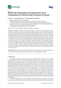
Fig. 1. Isotopic Approximation of curve sin3 (x2 ) − cos3 (y 2 ) = 0 with Core 2.

As an illustration of ENC applications, Figure 1 shows the curve f (x, y) = sin3 (x2 ) − cos3 (y 2 ) = 0 approximated by Core 2, using a recent algorithm [16]. Here sinn , cosn means we use the first n terms of their Taylor expansions. Our computation in the left figure stops once the isotopy-type is determined; in the right figure, we continue to a user-specified Hausdorff distance. Until recently, most exact computation on algebraic curves and surfaces are based on strong algebraic techniques such as resultant computation (e.g., [1]). In ENC, our main techniques are evaluation and domain subdivision (such subdivision boxes are seen in Figure 1). Superficially, this resembles the traditional numerical approaches, but ENC can provide the topological guarantees [16, 27] that is normally only associated with algebraic algorithms. ENC algorithms have many advantages: adaptive complexity, relatively easy to implement, and locality (i.e., we can restrict computational effort to a local region, as in Figure 1). §3. Goals of this Paper. There are three main motivations. The first is the desire to increase the modularity, extensibility and maintainability of Core Library. These are standard concerns of software engineering, but we shall discuss their unique manifestations in an ENC software. The second is efficiency: the centerpiece of any ENC library is a complex “poly-algorithm” (i.e., a suite of complementary algorithms that work together to solve a problem) to evaluate a numerical expression [15]. The optimal design of this poly-algorithm is far from understood, as we will see much room for improvement. The third is the desire to introduce transcendental computation into the context of ENC. As there are no constructive zero bounds for general transcendental expressions,

The Design of Core 2

5

we must intermix Level 2 with Level 3 accuracy (cf. (1)). Finally, our redesign is constrained to preserve the simple numerical accuracy API of Core Library as illustrated y (1), and to be backward compatible with Core 1. §4. Overview. Section 2 reviews the original design of Core Library and discusses the issues. Sections 3 and 4 present (resp.) the new design of the main C++ classes for expressions and bigFloats. Section 5 describes new facilities to make Expr extensible. We conclude in Section 6. Many topics in this paper appear in greater detail in the Ph.D. thesis [8] of one of the authors. The source code for all experiments reported here are found in the subdirectory progs/core2paper, found in our open source (QPL license) Core 2 distribution [7]. Experiments are done on an Intel Core Duo 2.4 GHz CPU with 2 GB of memory. The OS is Cygwin Platform 1.5 and compiler is g++-3.4.4.

inria-00519591, version 1 - 20 Sep 2010

2

Review of Core Library, Version 1

The Core Library features an object-oriented design, implemented in C++. A basic goal of the Core Library is to make ENC techniques transparent and easily accessible to (non-specialist) programmers through a simple numerical accuracy API (illustrated by (1)). User convenience is high priority because we view Core Library as a tool for experimentation and rapid prototyping. There are three main subsystems in Core 1: the expression class (Expr), the real number class (Real) and the big float number class (BigFloat). These are number classes, built over standard big number classes (BigInt, BigRat) which are wrappers around corresponding types from GNU’s multiprecision package GMP. The Expr class provides the critical functionalities of ENC. An instance of Expr is a directed acyclic graph (DAG) representing a numerical constant constructed from arbitrary real algebraic number constants. In the following, we raise some issues in the old design of the Expr and BigFloat classes. – Some critical facilities in Expr should be modularized and made extensible. Specifically, the filter and root bound facilities have grown considerably over the course of development and are now hard to maintain, debug, or extend. – The main evaluation algorithm (the “poly-algorithm” in the introduction) of Expr has three co-recursive subroutines. The old design does not separate their roles clearly, and this can lead to costly unnecessary computations. – Core 1 supports only algebraic expressions. An overhaul of the entire design is needed to add support for non-algebraic expressions. – Currently, users cannot easily add new operators to Expr. E.g., it is useful to add diamond operator [5], product, summation (see below), etc. Next consider the BigFloat class. It is used by Expr to approximate real numbers, and is the workhorse for the library. It is implemented on top of BigInt from GMP. The old BigFloat is represented by a triple hm, err, ei of integers, representing the interval [(m − err)B e , (m + err)B e ] where B = 214 is the base. We say the bigfloat is normalized when err < B and exact when err = 0. The following issues arise:

6

Yu, Yap, Du, Pion, and Br¨ onnimann

inria-00519591, version 1 - 20 Sep 2010

– The above representation of BigFloat has performance penalty as we must do frequent error normalization. Some applications do not need to maintain error. E.g., in self-correcting Newton-type iterations, it is not only wasteful but may fail to converge unless we zero out the error by calling makeExact. Users can manually call makeExact but this process is error-prone. – Our BigFloat assumes that for exact bigfloats, the ring operations (+, −, ×) are computed exactly. This is important for ENC but we see situations below where this is undesirable and the IEEE model of round-off is preferable. √ – The old BigFloat supports only {+, −, ∗, /, 2 }. For Expr to support transcendental functions such as exp, sin, etc., we need their BigFloat analogues (recall ingredient (a) in ¶2). This implementation is a major effort, and the correct rounding for transcendental functions is quite non-trivial [21]. To bring out these performance penalties, we compare our old BigFloat implementation of sqrt against MPFR [11]: Core 1 was 25 times slower as seen in Figure 8. The MPFR package satisfies all three criteria above. A key feature of MPFR is its support of the IEEE rounding modes (the “R” in MPFR refers to rounding). Hence a critical decision of Core 2 was to capitalize on MPFR.

3

Redesign of the Expr Package

We first focus on expressions. The goal is to increase modularity and extensibility of expression nodes, and also to improve efficiency. 3.1

Incorporation of Transcendental Nodes

What is involved in extending expressions to transcendental operators? In Core 1, we classify nodes in Expr into rational or irrational ones as such information is critical for root bound computation. We now classify them into integer, dyadic, rational, algebraic, and transcendental. A node is transcendental if any of its descendants has a transcendental operator (e.g., a leaf for π = 3.1415 . . ., or a unary node such as sin(·)). This refined classification of nodes are exploited in root bounds. There is a natural total ordering on these types, and the type of a node is the maximum of the types in descendant nodes. As transcendental expressions do not have root bounds, we introduce a user-definable global value called escape bound to serve as their common root bound. 3.2

New Template-based Design of ExprRep

The Expr class in Core 2 is templated, unlike in Core 1. It remains only a thin wrapper around a “rep class” called ExprRep, which is our focus here. §5. ExprRep and ExprRepT. The filter and root bound facilities were embedded in the old ExprRep class. We now factor them out into two functional modules: Filter and Rootbd. The Real class (see Section 2), which was already an independent module, is now viewed as an instance of an abstract number module called Kernel. The role of Kernel is to provide approximate real values. We introduce the templated classes ExprT and ExprRepT, parametrized by these three modules:

The Design of Core 2

7

template class ExprT; template class ExprRepT;

inria-00519591, version 1 - 20 Sep 2010

Now, Expr and ExprRep are just typedefs: typedef ExprT Expr; typedef ExprRepT ExprRep; The actual template arguments for Rootbd, Filter, and Kernel for Expr are passed to ExprRep, ExprT, and ExprRepT. The benefit of this new design is that now we can replace Filter, Rootbd or Kernel at the highest level without any changes in ExprRep, ExprT or ExprRepT. We see here that the default Expr class in Core 2 uses the k-ary BFMSS root bounds [5, 26] and the new BigFloat2 kernel (below). But users are free to plug in other modules. E.g., one could substitute a better filter and root bound for division-free expressions. This design of Expr follows the “delegation pattern” in Object-Oriented Programming [32]: the behavior of Expr is delegated to other objects (filters, etc). §6. ExprRepT class hierarchy. The class ExprRepT defines abstract structures and operations which are overridden by its subclasses. This hierarchy of subclasses is shown in Figure 2. ExprRepT

BinaryOpRepT

ConstOpRepT

UnaryOpRepT

AnaryOpRepT

CbrtRepT

AddSubRepT

ConstDoubleRepT

MulRepT

ConstFloatRepT

NegRepT

DivRepT

ConstIntegerRepT

RootRepT

ConstLongRepT

SqrtRepT

ConstPolyRepT

DiamondRepT

ConstRationalRepT

ProductRepT

ConstULongRepT

SumRepT

Fig. 2. ExprRepT Class hierarchy

There are four directly derived classes, corresponding to the arities of the operator at the root of the expressions: constants, unary, binary, and anary operators. Each of them has further derived classes – for instance, the binary operator class is further derived into three subclasses corresponding to the four arithmetic operators (AddSubRepT, MulRepT, DivRepT). The introduction of anary operators is new. An anary operator is one without a fixed arity, such as

8

Yu, Yap, Du, Pion, and Br¨ onnimann

Pn summation i=1 ti . Another is the diamond Pn operator 3(a0 , . . . , an , i) to extract the ith real root of a polynomial p(x) = i=0 ai xi [5] where ai ’s are expressions. §7. Memory layout of ExprRepT. Size of expression nodes can become an issue (see Section 5). Our design of ExprRepT optimizes the use of space (see Figure 3(a)). Each ExprRepT node has three fields filter, rootbd and kernel. Here, filter is stored directly in the node, while rootbd and kernel are allocated on demand, and only pointers to them are stored in the node. This is because the filter computation will always be done, but root bound and high precision approximations (from kernel) may not be needed. No memory will be allocated when they are not needed. The memory layout of ExprRepT is shown in Figure 3(b). E.g., a binary ExprRepT node uses a total of 48 bytes on a 32-bit architecture. The field cache is added to cache important small but potentially expensive information such as sign, uMSB, lMSB. The field numType is used for node classification.

inria-00519591, version 1 - 20 Sep 2010

ExprRep

ExprRepT

_filter

Filter

Filter

d_e,...

_rootbd

Rootbd

Real

_kernel Kernel

(a)

Field name Size in bytes Dynamic type information 4 Reference counter 4 Operands : Node * [arity] 4×arity Filter filter 16 Kernel * kernel 4 Rootbd * rootbd 4 Cache * cache 4 int numType 4 (b)

Fig. 3. (a) Comparing ExprRep and ExprRepT. (b) Layout in 32-bit architecture.

§8. Some Timings. We provide two performance indicators after the above redesign. In Figure 4(a), we measure the time to decide the sign of determinants, with and without (w/o) the filter facility, in Core 1 and Core 2. The format ‘N ×d×b’ in the first column indicates the number N of matrices, the dimension d of each matrix and the bit length b of each matrix entry (entries are rationals). Interestingly, for small determinants, the filtered version of Core 1 is almost twice as fast. All times are in microseconds. MATRIX Core 1.7 Time with (w/o) filter 9 (621) 26 (1666) 449 (1728) 1889 (3493) 4443 (6597) 8100 (11367)

1000x3x10 1000x4x10 500x5x10 500x6x10 500x7x10 500x8x10

Core 2.0 Time with (w/o) filter 19 (232) 43 (530) 204 (488) 597 (894) 1426 (1580) 2658 (2820)

Speedup 0.5 0.6 2.2 3.2 3.1 3.0

(2.7) (3.1) (3.5) (3.9) (4.2) (4.0)

bit length L Core 1 1000 0.82 2000 6.94 8000 91.9 10000 91.91

Core 2 Speedup 0.59 1.4 1.67 4.2 11.63 7.9 30.75 3.0

(b)

(a) Fig. 4. (a) Timing filter facility (b) Timing root Bound facility

In Figure 4(b), weptest the new root bound facility by performing the com√ √ √ x + y + 2 xy where x, y are b-bit rational numbers. As parison x + y : this expression is identically zero, filters do not help and root bounds will always be reached.

The Design of Core 2

3.3

9

Improved Evaluation Algorithm

Since the evaluation algorithm is the centerpiece of an ENC library, it is crucial to tune its performance. §9. Algorithms for sign(), uMSB() and lMSB(). Core 1 has two main evaluation subroutines, computeApprox() and computeExactSign() (see [15]). The former computes an approximation of the current node to some given (composite) precision bound. The latter computes the sign, upper and lower bounds on the magnitude of the current node. These three values are maintained in Expr as sign(), uMSB() and lMSB(). In Core 1, computeExactSign() computes them simultaneously using the rules in Table 5.

inria-00519591, version 1 - 20 Sep 2010

E Constant x

E1 ± E2

E1 × E2 E1 ÷ E2 √ k E1

Case if E1 .sgn() = 0 if E2 .sgn() = 0 if E1 .sgn() = ±E2 .sgn() if E1 .sgn() 6= ±E2 .sgn() and E1− > E2+ if E1 .sgn() 6= ±E2 .sgn() and E1+ < E2− otherwise

E.sgn() E+ E− sign(x) ⌈log2 x⌉ ⌊log2 x⌋ ±E2 .sgn() E2+ E2− E1 .sgn() E1+ E1− + + E1 .sgn() max{E1 , E2 } + 1 max{E1− , E2− } E1 .sgn() max{E1+ , E2+ } E1− − 1 ±E2 .sgn() max{E1+ , E2+ } E2− − 1 unknown max{E1+ , E2+ } unknown E1 .sgn() ∗ E2 .sgn() E1+ + E2+ E1− + E2− − − + E1 .sgn() ∗ E2 .sgn() El1+ − Em E 2 2 j1 − Ek + − E1 /k E1 /k E1 .sgn()

Fig. 5. Recursive rules for computing sign, uMSB, lMSB.

There are two “unknown” entries in Table 5. In these cases, computeApprox() will loop until the sign is determined, or up to the root bound. To compute such information, we recursively compute sign and other information over the children of this node, whether needed or not. This can be unnecessarily expensive. In Core 2, we split the 2 routines into five co-recursive routines in ExprRepT: get sign(), get uMSB(), get lMSB(), refine() and get rootBd(). Depending on the operator at a node, these co-routines can better decide which information from a child is really necessary. The structure of these algorithms are quite similar, so we use get sign() as an example: Sign Evaluation Algorithm, get sign(): 1. Ask the filter if it knows the sign; 2. Else if the cache exists, ask if sign is cached; Note: the cache may contain non-sign information 3. Else if the approximation ( kernel) exists, ask if it can give the sign; 4. Else if the virtual function compute sign() returns true, return sgn() (sign is now in the cache); 5. Else call refine() (presented next) to get the sign. Thus it is seen that, for efficiency, we use five levels of computation to determine sign: filter, cache, kernel, recursive rules (called compute sign()), and

10

Yu, Yap, Du, Pion, and Br¨ onnimann

refine(). Note that we do not put the cache at the first level. We do not even cache the sign, uMSB and lMSB information when the filter succeeds because a Cache structure is large and we try to avoid costly memory allocation. The object oriented paradigm used by the above design is called the “template method pattern” [12, p. 325]: define the skeleton of an algorithm in terms of abstract operations which is to be overridden by subclasses to provide concrete behavior. In the derived classes of ExprRepT, it is sufficient to just override the virtual function compute sign() when appropriate. For example, MulRepT may override the default compute sign() function as follows:

inria-00519591, version 1 - 20 Sep 2010

1 2 3

v i r t u a l bool c o m p u t e s i g n ( ) { s i g n ( ) = f i r s t −>g e t s i g n ( ) ∗ s e c o n d−>g e t s i g n ( ) ; return true ; }

§10. Algorithm for refine(). As seen in the get sign() algorithm, if the first four levels of computation fail, the ultimate fall-back for obtaining sign (and also for lower bounding magnitude) is the refine() algorithm. We outline this key algorithm to obtain sign via refinement: 1. If the node is transcendental, get the global escape bound. Otherwise, compute the constructive root bound. 2. Take the minimum of the bound from step 1 and the global cutoff bound. 3. Compute an initial precision. If an approximation exists, use its precision as the initial precision. Otherwise use 52 bits instead which is the relative precision that a floating-point filter can provide. 4. Initialize the current precision to the initial precision. Then enter a for-loop that doubles the current precision each time, until the current precision exceeds twice the bound computed in step 2. 5. In each iteration, call a approx() (see below) to approximate the current node to an absolute error less than the current precision. If this approximation suffices to give a sign, return the sign immediately (skip the next step). 6. Upon loop termination, set the current node to be zero. 7. Check if the termination was caused by reaching the escape bound or cutoff bound. If so, append zero assertion to a diagnostic file in the current directory. This assertion says that “the current node is zero”. §11. Conditional Correctness. The cutoff bound in the above refine() algorithm is a global variable that is set to CORE INFTY by default. While escape bound affects only transcendental nodes, the cutoff bound sets an upper bound on the precision in refine() for all nodes. Thus it may override computed zero bounds and escape bounds. During program development, users may find it useful to set a small cutoff bound using set cut off bound(). Thus, our computation is correct, conditioned on the truth of all the zero assertions in the diagnostic file. §12. Computing Degree Bounds. In the refine() algorithm above, the first step is to compute a constructive root bound. Most constructive root bounds need an upper bound on the degree of an algebraic expression [15]. For

The Design of Core 2

11

radical expressions, a simple upper bound √ is obtained as the product of all the degrees of the radical nodes (a radical node k E has degree k). A simple recursive rule can obtain the degree bound of E from the degree bounds of its children (e.g., [14, Table 2.1]). But this bound may not be tight when the children share nodes. The only sure method is to traverse the entire DAG to compute this bound. To support this traversal, in Core 1 we store an extra flag visited with each ExprRep. Two recursive traversals of the DAG are needed to set and to clear these flags, while computing the degree bound. To improve efficiency, we now use the std::map data structure in STL to compute the degree bound: we first create a map M and initialize the degree bound D to 1. We now traverse the DAG, and for each radical node u, if its address does not appear in M , we multiply its degree to the cumulative degree bound D and save its address in M . At the end we just discard the map M . This approach requires only one traversal of the DAG.

inria-00519591, version 1 - 20 Sep 2010

3.4

Improved Propagation of Precision

An essential feature of precision-driven evaluation is the need to propagate precision bounds [15]. Precision propagation can be illustrated as follows: if we want to evaluate an expression z = x + y to p-bits of absolute precision, then we might first evaluate x and y to (p + 1)-bits of absolute precision. Thus, we “propagate” the precision p at z to precision p + 1 at the children of z. This propagation is correct provided x and y have the same sign (otherwise, p + 1 bits might not suffice because of cancellation). In general, we must propagate precision from the root to the leaves of an expression. In Core 1, we use a pair [a, r] of real numbers that we call “composite precision” bounds. If x, x e ∈ R, then we say x e is an [a, r]-approximation of x (written, “e x ≈ x[a, r]”) if |e x − x| ≤ 2−a or −r |e x − x| ≤ |x|2 . If we set a = ∞ (resp., r = ∞), then x e becomes a standard relative r-bit (resp., an absolute a-bit) approximation of x. It is known that a relative 1-bit approximation would determine the sign of x; so relative approximation is generally infeasible without zero bounds. The propagation of composite bounds is tricky, and various small constants crop in the code, making the logic hard to understand and maintain (see [25]). Our redesign offers a simpler and more intuitive solution in which we propagate either absolute or relative precision, not their combination. §13. Algorithms for r approx() and a approx(). Core 1 has one subroutine computeApprox() to compute approximations; we split it into two subroutines a approx() and r approx(), for absolute and relative approximations (respectively). Above, we saw that refine calls a approx(). There are two improvements over Core 1: first, propagating either absolute or relative precision is simpler and can avoid unnecessary precision conversions. Second, the new algorithms do not always compute the sign (which can be very expensive) before approximation. §14. Overcoming inefficiencies of Computational Rings. Another issue relates to the role computational rings in ENC (see §16 in [35]). This

12

Yu, Yap, Du, Pion, and Br¨ onnimann

inria-00519591, version 1 - 20 Sep 2010

is a countable set F ⊆ R that can effectively substitute for the uncountable set of real numbers. To achieve exact computation, F needs a minimal amount of algebraic structures [35]. We axiomatize F to be a subring of R that is dense in R, with Z as a subring. Furthermore, the ring operations together with division by 2, and comparisons are effective over F. BigFloats with exact ring operations is a model of F, but IEEE bigFloats is not. For computations that do not need exactness, the use of such rings may √ incur√performance penalty. To demonstrate this, suppose we want to compute 2 · 3 to relative p-bits of√precision. √ We describe two methods for this. In Method 1, we approximate 2 and 3 to relative (p + 2)-bits, then perform the exact multiplication of these values. In Method 2, we proceed as in Method 1 except that the final multiplication is performed to relative (p + 1)-bits. The timings (in microseconds) are shown in Figure 6. We use loops to repeat the experiment since the time for single runs is short. It is seen that Method 2 can be much more efficient; this lesson is incorporated into our refinement algorithm. Precision 10 100 1000 10000 100000

Loops Method 1 Method 2 Speedup 1000000 345 191 45% 100000 60 46 23% 10000 72 71 1% 1000 267 219 18% 100 859 760 12%

Fig. 6. Timing for computing

4

√

2·

√

3 w/ and w/o exact multiplication.

Redesign of the BigFloat system

The BigFloat system is the “engine” for Expr, and Core 1 implements our own BigFloat. In Section 2, we discussed several good reasons to leverage our system on MPFR, an efficient library under active development for bigFloat numbers with directed rounding. Our original BigFloat plays two roles: to implement a computational ring [35] (see section section 3.4), and to provide arbitrary precision interval arithmetic [24]. Computational ring properties are needed in exact geometry: e.g., to compute implicit curve intersections reliably, we can evaluate polynomials with exact BigFloat coefficients, at exact BigFloat values, using exact ring operations. Interval arithmetic is necessary to provide certified approximations. For efficiency, Core 2 splits the original BigFloat class into two new classes: (1) A computational ring class, still called BigFloat. (2) An interval arithmetic class called BigFloat2, with each interval represented by two MPFR bigFloats. This explains3 the “2” in its name. 4.1

The BigFloat Class as Base Real Ring

The new class BigFloat is based on the type mpfr t provided by MPFR. MPFR follows the IEEE standard for (arbitrary precision) arithmetic. The results of 3

Happily, it also coincides with the “2” in the new version number of Core Library.

The Design of Core 2

13

arithmetic operations are rounded according to user-specified output precision and rounding mode. If the result can be exactly represented, then MPFR always outputs this result. E.g., a call of mpfr mul(c, a, b, GMP RNDN) will compute the product of a and b, rounding to nearest BigFloat, and put the result into c. The user must explicitly set the precision (number of bits in the mantissa) of c before calling mpfr mul(). To implement the computational ring BigFloat, we just need to automatically estimate this precision. E.g., we can use the following:

inria-00519591, version 1 - 20 Sep 2010

Lemma 1. Let fi = (−1)si · mi · 2ei (for i = 1, 2) be two bigFloats in MPFR, where 1/2 ≤ mi < 1 and the precision of mi is pi . To guarantee that all bits in the mantissa of the sum f = f1 ± f2 is correct, it suffices to set the precision of f to ½ 1 + max{p1 + δ, p2 } if δ ≥ 0 1 + max{p1 , p2 − δ} if δ < 0 where δ = (e1 − p1 ) − (e2 − p2 ). Similarly, for multiplication, it suffices to set the precision of f to be p1 + p2 in computing f = f1 · f2 . See [8] for a proof. While this lemma is convenient to use, it may over-estimate the needed precision. In binary notation, think of the true precision of c as the minimum number of bits to store the mantissa of c. Trailing zeros in the mantissa contributes to over-estimation. To avoid this, we provide a function named mpfr remove trailing zeros() whose role is to remove the trailing zeros. In an efficiency tradeoff, it only removes zeros by chunks (chunks are determined by MPFR’s representation). To understand the effect of overestimation, we conduct Qn an experiment in which we compute the factorial F = i=1 i using two methods: In Method 1, we initialize F = 1 and build up the product in a for-loop with i = 2, 3, . . . , n. In the i-th loop, we increase the precision of F using Lemma 1, then call MPFR to multiply F and i, storing the result back into F . In Method 2, we do the same for-loop except that we call mpfr remove trailing zeros() on F after each multiplication in the loop. Pn Instead of F , we can repeat the experiment with the arithmetic sum S = i=1 i. The speedup for the second method over the first method is shown in Figure 7 (time in microseconds, precision in bits).

n

Q F = n i=1 i trailing zeros no zeros (prec/msec) (prec/msec)

Pn S= i=1 i trailing zeros no zeros (prec/msec) (prec/msec)

102 575/0 436/0 102/0 103 8979/0 7539/0 1002/0 104 123619/62 108471/47 10002/15 105 1568931/9219 1416270/8891 100002/437 106 timeout timeout 1000002/57313

31/0 31/0 31/16 31/110 63/1078

Fig. 7. Timing for computing F and S w/ and w/o removing trailing zeros.

14

Yu, Yap, Du, Pion, and Br¨ onnimann

§15. Benchmarks of the redesigned BigFloat. By adopting MPFR, our BigFloat class gains many new functions such as cbrt() (cube root) and the elementary functions (sin(), log(), etc). The performance of the BigFloat is also greatly improved. We compared the performance √ of Core 1 and Core 2 on sqrt() using the following experiment: compute i for i = 2, . . . , 100 with precision p. The timing in Figure 8 show that Core 2 is about 25 times faster, thanks purely to MPFR. Precision Core 1 Core 2 Speedup 1000 25 1 25 10000 716 32 22 100000 33270 1299 25

inria-00519591, version 1 - 20 Sep 2010

Fig. 8. Timing comparisons for sqrt().

4.2

The Class BigFloat2

BigFloat2 is the second class split off from the original BigFloat. An instance of BigFloat2 is just an interval represented by a pair of bigFloat numbers. This representation can be less efficient than the original BigFloat by a factor of 2 (in the worst case), both in speed and in storage. But this loss in efficiency is compensated by ease of implementation, and in sharper error bounds, which may be beneficial in non-asymptotic situations. In the future, we may also experiment with a bigfloat class using a midpoint-radius representation using MPFR. This class is also useful for ENC applications (e.g., in meshing algorithms of the kind producing Figure 1).

5

Extending the Expr Class

We provide facilities for adding new operators to Expr. Core 2 uses such facilities to implement the standard elementary functions. Future plans include extending elementary functions to all hypergeometric functions, following the analysis in [8, 9]. We give two examples of how users can use these facilities for their own needs. We refer to Zilin Du’s thesis [8] for more details about these facilities. 5.1

Summation Operation for Expr

When an Expr is very large, we not only lose efficiency (just to traverse the DAG) but we often run out Pnof memory. Consider the following code to compute the harmonic series H = i=1 1i : Expr harmonic ( i n t n ) { Expr H ( 0 ) ; f o r ( i n t i =1; i