THE LMK ALGORITHM WITH TIME-VARYING FORGETTING FACTOR FOR ADAPTIVE SYSTEM IDENTIFICATION IN ADDITIVE OUTPUT-NOISE 0. Tanrikulu and A . G. Constantinides Signal Processing Section, Department of Electrical and Electronic Engineering, Imperial College of Science, Technology and Medicine, London SW7 2BT, UK.
[email protected] ABSTRACT Adaptive algorithms are succeptible to noise signals due to the perturbation of the gradient direction. Depending upon the statistics of the noise, various cost functions can be minimised. The Least Mean Kurtosis (LMK) adaptive algorithm is a stochastic gradient approach that uses the kurtosis of the error signal. Depending upon the noise distribution, the forgetting factor used in the LMK algorithm must be chosen optimally. In this paper, a version of LMK is presented, in which the forgetting factor is made time-varying such that if the output-noise distribution is unknown, which is almost always the case in practice, the algorithm will tune its forgetting factor in sympathy with the noise distribution. Hence the proposed algorithm is more flexible than the Least Mean Square (LMS) and Least Mean Fourth (LMF) adaptive algorithms under noisy conditions. 1. INTRODUCTION
There is considerable amount of research activity dedicated to adaptive algorithms that use non mean-square cost functions. Important applications are in blind equalisation [5] and system identification [14, 4, 31. In blind equalisation, cost functions with higher-order moments of the equaliser output are used in order to correctly identify the phase characteristics of the channel. Many significant contributions exist but we would like to mention the work by Shalvi and Weinstein [S, 91 which uses the same higher-order statistical measure; the kurtosis, that the LMK algorithm is based upon. In the area of adaptive system identification (or adaptive interference reduction which is very similar), general odd-symmetric functions of the error signal are used in the update of the adaptive coefficients [4, 31. Walach and Widrow [14] carried out a detailed study of a family of adaptive algorithms where the even-order moments of the error signal are used as cost functions. They have shown that if the output-noise distribution is sub-Gaussian, minimising higher-order moments of even degree produce lower misadjustment than minimising the mean-squared error. On the other hand, if the output-noise distribution is Gaussian or super-Gaussian, mean-square error cost function is more advantageous to use. Some current work on the normalisation of such algorithms can be found in [7, 21.
0-7803-3 192-3/96 $5.0001996 IEEE
The Error Performance Surfaces (EPS) defined by the kurtosis or the fourth-order moment are unimodal Ell],but the stationary points may be more difficult to converge to since the EPSs are much more flatter than the mean-square error surface. To ensure the existence of well defined minima, Tugnait [13] minimised the square root of the absolute value of the kurtosis for system identification in a block-based scheme. Although the stationary points of this cost function are well-defined, local minima also exists. Recently, Amblard and Brossier [l] have shown that recursive estimation of the kurtosis produces lower variance estimates than block based estimation. The LMK algorithm uses the kurtosis of the error signal to update the adaptive coefficients [12]. The EPS of the LMK algorithm is unimodal. Moreover, as long as the additive output-noise signal exists, the stationary point of the error surface is a well defined minimum [ll].The misadjustment of the LMK algorithm is dependant on the output-noise statistics and can be minimised by choosing an appropriate value for the forgetting factor. In this paper, we present a variant of the LMK algorithm (LMK-VP), where the forgetting factor is made time-varying so that the optimal value of this parameter is obtained at the steady-state. 2. LMK ADAPTIVE ALGORITHM
The block-diagram for adaptive system identification in additive output-noise is illustrated in Figure 1 where, U, is the input signal, d, = uzh,t is the desired signal, h,t is the vector that contains the parameters of the unknown system and w n is the additive output-noise.
Figure 1: Adaptive system identification in output noise. The error signal is defined as
1850
e,
A = W
n
- U Tn V n
where
A
vn = hn
- hopt
(2)
is the weight error vector, U n = [ U n U n - l . . . un-N+1IT and hn = [hn,ohn,l . . . h n , ~ - 1 I T .[.IT denotes vector transposition and N is the number of adaptive coefficients. The following assumptions are put into effect; AI) Statistically, un and wn are strictly stationary and zeromean. A2) tun and U,, are statistically independent. A3) wn is white with bounded moments and has a symmetrical probability density function. A4) hopt is time-invariant.
Provided that 0 < /3 < 1, which is already an exponential stability constraint for the recursive error power estimation, (10) is positive. Experiment I The accuracy of (9) is valildated by identifying a IO-th order arbitrary Finite Impulse Response (FIR) system. The initial condition is ho = 0. The input signal, U,,, is zero-mean, white and uniformly distributed with unity power. The noise sign(a1, tun, is white Gaussian distributed and SNR=lOdB. Thle experimenl, consisted an average of 100 trials and the rnisadjustment is computed at the steady-state from (8). The theoretical value of the misadjustment is computed from (9). The results are shown in Figure 2. In further experiments with other noise distribu-
Consider the negated kurtosis of the error signal -5,
-10
where E{.} is the statistical expectation operator. The gradient vector corresponding to (3) is
For algorithm construction, E { e i } in (4) must be replaced with an approximation that can be computed in real-time [lo]. For this purpose, we define the alternative gradient vector V"J, = -4~{(30,2,,e, - e:)un) (5) where q:,n = P d . , n - l + (1 - P ) e ; , o < P < 1 (6) where P is the f o r g e t t i n g factor that controls the memory of the error power estimator. By using Al-A3, it can be shown that V"J, = 0 when vn = 0 and thus vn = 0 is a stationary point on the EPS. Furthermore, provided that un has a non-Gaussian distribution, v,, = 0 is the only stationary point and it is a minimum [ll]. The gradientdescent based update equation of the LMK algorithm is hn+l = hn
+ 4p(3d,,en - ei)Un
,
,
,
,
I
Figure 2: Misadjustment vs. output-noise.
,
I
,
7
--
,I
P for Gauss:an distributed
tions, it is observed that (9) is an accurahe approximation of the misadjustment of the LMK algorithm. Definition Let {W,,} be a stationary stochastic process with an associated random variable wn. Define the normalised fourth-order moment
(7)
where L,I is the adaptation gain. A When of = E{&} # 0, we can define the misadjustment as in [14]
n:
A E'{W:} = -E:z{wZ}
The distribution of tu, is term recpectivelly sub-Gaussian, Gaussian or super-Gaussian if n is less than, equal to or greater than 3.0. The normalised misadjustment, which is defined as
Therefore, if limn+oo h, = hopt, then M = 0. In [ll],an approximate expression for the misadjustment of the LMK algorithm is obtained as
(9) A
A
where ( : = E{wk}, and €2 = E{wE}. Note that, (9) is obtained by ignoring statistical expectations that contain third and higher-order products of the elements of V n . This corresponds to a linearisation of the update equation around the optimum and it does not violate the positive definite nature of E { v , v ~ } . Indeed, (9) is a positive quantity which can be easily shown by rewriting it as
M = pNE{u2,} E{(3/302,Wn - (2 - 3p)W:)') 3 ( 1 - P)o&
(10)
is shown in Figure 3 for various noise distributions. Clearly, for sub-Gaussian noise distributions (i.e. Bernoulli; K = 0.9 and Uniform; n: = 1.8) p must be small. On the other hand, for Gaussian and super-Gaussian distributions (i.e. Laplacian; K = 6.0 and Pearson's; K = 5 . 0 ) , there are well-defined values of p for minimum misadjustment. IC; is important to point out that if /3 = 0, then the gradient vector in (5) reduces to the gradient vector in the Lead Mean-Fourth (LMF) adaptive algorithm. Therefore, p = 0 in Figure 3 corresponds to the normalisecl misadjustm ent of the LMF algorithm. Hence, in order to achieve optiimal steady-state behaviour, p must be allowed to be time-varying. This is discussed in the next section.
1851
,-3o-
-,L: LAPLACIAN
3
-.P PEARSONs
in i E [nL-L, . . . , nL- 13. These are equivalent to hypothesising predefined states of convergence in the current block of data with which the forgetting factor will be updated. The approximation (18) essentially reduces the update in (15) to a fist-order recursion in P. This can be seen by writing the error under the approximations in (17),(18).
, ,,‘
e, x ~ ~ - 4 ~ ( 3 ~ ~ L - L ( u ” , w t , ) 2 u t - 1 + 2 w ~ - l ) u r u l - (19) l
Around the optimum we can also assume that the timevarying forgetting is statistically independent of the input and noise signals [ll]. By using (17),(18) and (19) in (15) and taking the limit we can obtain
Figure 3: Normalised misadjustment vs.
P. by using (19) in (15). The LMK-VP algorithm is used in the following experiment Experiment I1 The unknown system is chosen as h,t = [1.000 0.857 - 0.756 1.491 0.642 - 0.195 0.196 0.820IT. The input signal is white and uniformly distributed in [-1,1]. is 5dB and the block The SNR = 10loglo(E{d~}/E{w~}) size, L, is 500. The experiment is repeated 20 times with 3 . 5 ~ 1 0iterations ~ in each trial. The initial values of the forgetting factor and the other adaptation parameters are shown in Table 1. The asymptotical values of the forgetting
3. LMK-VP ALGORITHM
In the LMK-VP algorithm, the underlying ideas in variable step-size LMS algorithms [6] are used. Since the misadjustment of the algorithm is to be minimised, P is updated such that 8E{e2,1 - 0 -(13) 8Pn-1
This yields the update equation
Pn = Pn-l
+ ~E{(U:,,,-~ - e~-,)enen-luff-1un}
(14)
where p is a small positive real number. It can be easily shown that E{et} is convex with respect to P. Furthermore, the choice of p is not as crucial as it is in variable step-size LMS algorithms since we know that 0 < Pn < 1 must be satisfied for the estimation of the error power. If Pn is updated at each time instant, the recursive estimation of the error power will be in large error due to the fluctuations and thus, a block based update of P is more appropriate. Therefore, we use the update equation
Pnr. = P ~ L - L+
2
nL-1
(d,,-z
-e?-l)e,ec-lu?-lu,
Laplacian
Noise Bernoulli Laplacian
i E [nL - L, . . . ,nL - 11. Note that the adaptive coeffcients are updated as in (7). We now obtain an approximate expression for the asymptotical value of Pn;
w. For this purpose, we take Vn,O < Pn < 1 which is similar to the assumption that the step-size, pnrof a variable stepsize LMS algorithm always satisfies pn E (0,2/3tr[R]) [SI, where R = E{unuIf}. We will proceed heuristically and make some assumptions on the asymptotical values of certain terms in (15). If the algorithm is convergent to a small ball around the optimum, we have
d,,-z =
0.1
I 5.0~10-~
(15)
+ (1 - AL-L)$-~, (16)
e,-1 x w,-1
I
factor are shown in Table 2. It is not possible to compute
oo for the Bernoulli distribution, since the numerator and the denominator of (20) are identically equal to zero for this case. However, the normalised misadjustment curve in Figure 3 for this distribution indicates that the forgetting factor has converged to its anticipated value.
where L is the Mock-size and the error power estimation is performed as
v,-1 x 0
0.0
Table 1: Adaptation parameters for the LMK-VP algorithm for different noise distributions.
*=nL-L
u & - ~= P n ~ - ~ a : , , - 3
11
(17) (18)
PEXP 3.20~10-‘ 0.715
m NA 0.709
Table 2: Experimental, PEXP, and theoretical velues of the asymptotical value of the forgetting factor. NA; Not applicable The gradient type update of P in (15) generally yields slow convergence and hence not practical. A Newton type u p date which involves 82E{e:}/8P:-1 is more appropriate. In this case we have the update
(21) i E [nL - L, . . . , nL - 11 where, X is a safety factor to avoid very small denominator values. Experiment I11 The unknown system is chosen as hop*= [0.1 0.2 0.3 0.4 0.5 0.4 0.3 0.2 0.1IT [14]. The input signal is
1852
white and uniformly distributed in [-1,1]. The SNR is -5dB, L = 100, and X = The results are averaged over 100 trials. The adaptation parameters are shown in Table 3.
.
, , . - ,
11
Bernoulli Gaussian
0.8
0.0
,
I 0.5 I lo-" I 0.5 I 3 . 0 ~ 1 0 - ~
Table 3: Adaptation parameters for the LMK-VP algorithm with block Newton type update.
The time variation of the forgetting factor and system mismatch, which is defined as the trace of the weight error corP relation matrix; SM = tr[v,vT] for Gaussian distributed noise case with time-varying and fixed /3 are shown in Figures 4-5. In Figure 4, the forgetting factor converges around the values we expect from Figure 3. In Figure 5, the advantage of using a time-varying forgetting factor is clearly visible. I 0.8
,
,
.
,
.
,
.
.
4. CONCLUSION!S
A time-varying version of the LMK algorithm is presented. The forgetting factor used in error power estimation is updated in a block fashion in order to minimise the misadjustment. It is observed that the forgetting factor converges around the anticipated values for differ'ent noise distributions. If the noise has a sub-Gaussian distribution, then the forgetting factor decreses around zero and the LMK-V/3 algorithm becomes similar to the LMF algorithm of Walach and Widrow. For Gaussian and super-Gaussian distributions, the optimum value of the forgetting factor is non-zero and can be converged to by using the proposed algorithm without any knowledge of tlhe noise distribution.
5. REFERENCES [l] P. 0. Amblard and J. M. Brossier. Adaptive estimation of the fourth-order cumulant of a white stochastic process. Signal Processing, 42( 1):37-43, Feb. 1995. [2] S. C. Douglas. A family of normalised LMS algorithms. IEEE Sig. Proc. Letters, 1(3):49-51, March 1994. [3] S. C. Douglas and E. T. H. Y . Meng. Normalised data nonlinearities for LMS adaptation. IEEE Trans. Sig. Proc., 42(6) :1352-1365. June 1994. [4] S. C. Douglas and E. yr. H. Y. Menig. Stochastic gradient adaptation under general err& criteria. IEEE Trans. Sig. Proc., 42(6):1335-1351, June 1994. S. Haykin. Adaptive Filter Theory. Englewood Cliffs, NJ: Prentice-Hall, 2-nd edition, 1991. V. J. Mathews and 2. Xie. A stochastic gradient adaptive filter with gradient adaptive step size. IEEE lrans. Sig. Proc., 41(6):2075-2087, June 1993. A. E. Cetin 0. Arikan and E. Erzin. Adaptive filtering for non-gaussian stable processes. IEEE Sig. Proc. Letters, 1(11):163-165, Nov. 1994. 0. Shalvi and E. Weinstein. New criteria for blind deconvolution of nonminiinum phase systems (channels). IEEE Trans. Inform. Theory, 36:312-321, Mar. 1990. 0. Shalvi and E. Weinrrtein. Super exponential methods for blind deconvolution. IEEE Trans. Inform. Theory, 39(2):504-519, Mar. 1993. V. Solo and X. Kong. Adaptive Signlo1 Processing Algorcthms: Stability and Performance. Englewood Cliffs, NJ: Prentice-Hall, 1995. 0. Tanrikulu. Adaptive signal processing algorithms with accelerated convergence and noise immunsty. PhD thesis, Imperial College, 1995. 0. Tanrikulu and A. C;. Constantinides. Least-mean kurtosis: A novel higher-order statistics based adaptive filtering algorithm. Electronics Letters, 30(3):189-190, Feb. 1994. J K. Tugnait. Stochastic system iidentification with noisy input using cumulant statistics. IEEE Trans. Automat. Contr., 37(4):476-485, Apr. 1992. E. Walach and B. Widrow. The Least Mean Fourth (LMF) adaptive algoritlhm and its family. IEEE Trans. Inform. Theory, 30(2):275-283, Mar. 1984.
,
-
0.8 1
0.1 -4 0.8
-;
GAUSSIAN
.
Figure 4: Time variation of the forgetting factor for Bernoulli distributed noise.
VARIABLE 0
-%O
02
0.4
0.6
0.8
1
12
1.4
NUMBER OF IERATIONS
1.6
1.8
2 10'
Figure 5: System mismatches for Bernoulli distributed noise with fixed and time-varying forgetting factor.
1853