The Poisson transform for unnormalised statistical models

arXiv:1406.2839v2 [stat.CO] 27 Nov 2014

The Poisson transform for unnormalised statistical models Simon Barthelmé, Nicolas Chopin Abstract Contrary to standard statistical models, unnormalised statistical models only specify the likelihood function up to a constant. While such models are natural and popular, the lack of normalisation makes inference much more difficult. Extending classical results on the multinomial-Poisson transform (Baker, 1994), we show that inferring the parameters of a unnormalised model on a space Ω can be mapped onto an equivalent problem of estimating the intensity of a Poisson point process on Ω. The unnormalised statistical model now specifies an intensity function that does not need to be normalised. Effectively, the normalisation constant may now be inferred as just another parameter, at no loss of information. The result can be extended to cover non-IID models, which includes for example unnormalised models for sequences of graphs (dynamical graphs), or for sequences of binary vectors. As a consequence, we prove that unnormalised parameteric inference in non-IID models can be turned into a semi-parametric estimation problem. Moreover, we show that the noise-contrastive estimation method of Gutmann and Hyvärinen (2012) can be understood as an approximation of the Poisson transform, and extended to non-IID settings. We use our results to fit spatial Markov chain models of eye movements, where the Poisson transform allows us to turn a highly non-standard model into vanilla semi-parametric logistic regression.

Unnormalised statistical models are a core tool in modern machine learning, especially deep learning (Salakhutdinov and Hinton, 2009), computer vision (Markov random fields, Wang et al., 2013) and statistics for point processes (Gu and Zhu, 2001), network models (Caimo and Friel, 2011), directional data (Walker, 2011). They appear naturally whenever one can best describe data as having to conform to certain features: we may then define an energy function that measures how well the data conform to these constraints. While this way of formulating statistical models is extremely general and useful, immense technical difficulties may arise whenever the energy function involves some unknown parameters which have to be estimated from data. The reason is that the normalisation constant (which ensures that the distribution integrates to one) is in most cases impossible to compute. This prevents direct application of classical methods of maximum likelihood or Bayesian inference, which all depend on the unknown normalisation constant. Many techniques have been developed in recent years for such problems, including contrastive divergence (Hinton, 2002; Bengio and Delalleau, 2009), 1

1 Relationship to prior work

2

noise-contrastive estimation (Gutmann and Hyvärinen, 2012) and various forms of MCMC for Bayesian inference (Møller et al., 2006; Murray et al., 2012; Girolami et al., 2013). The difficulty is compounded when unnormalised models are used for non-IID data, either sequential data, or data that include covariates. If the data form a sequence of length n, there are now n normalisation constants to approximate. In our application we look at models of spatial Markov chains, where the transition density of the chain is specified up to a normalisation constant, and again one normalisation constant needs to be estimated per observation. In the first Section, we show that unnormalised estimation is tightly related to the estimation of point process intensities, and formulate a Poisson transform that maps the log-likelihood of a model L (θ) into an equivalent cost function M (θ, ν) defined in an expanded space, where the latent variables ν effectively estimate the normalisation constants. In the case of non-IID unnormalised models we show further that optimisation of M (θ, ν) can be turned into a semi-parametric problem and adressed using standard kernel methods. In the second section, we show that the noise-contrastive divergence described in of Gutmann and Hyvärinen (2012) arises naturally as a tractable approximation of the Poisson transform, and that this new interpretation lets us extend its use to non-IID models. (Gutmann and Hyvärinen (2012) call the technique “noise-contrastive estimation”, but we use the term noise-contrastive divergence to designate the corresponding cost function.) Finally, we apply these results to a class of unnormalised spatial Markov chains that are natural descriptions of eye movement sequences.

1

Relationship to prior work

Some of the ideas we use here have appeared under different forms in classical statistics, machine learning and spatial statistics. The Poisson transform generalises the multinomial-Poisson transform developed by Baker (1994). It is also a special case of a general family of Bregman divergences introduced by Gutmann and ichiro Hirayama (2011), a special case of another family by Pihlaja et al. (2010), and finally can also be viewed as an empirical version of the generalised Kullback-Leibler divergence for unnormalised measures (Minka, 2005). Noise-contrastive learning is studied in Gutmann and ichiro Hirayama (2011), although the relationship between logistic regression and estimation has been noted in other places (for example, in the spatial statistics literature, see Baddeley et al., 2010, Baddeley et al., 2014). We go further here in showing that the divergence defined by NCL converges uniformly to the Poisson transform, giving it a new interpretation as an approximate likelihood rather than just a divergence. Mnih and Kavukcuoglu (2013) and Mnih and Teh (2012a) use the NCL technique in a class of non-IID unnormalised models. However, in the interest of computation time, they ignore normalisation constants. The results given here indicate clearly that neglecting normalisation constants leads in the general case

3

to non-convergent estimators, as illustrated in Section 4.1. Instead we develop a semi-parametric framework for non-IID estimation, which is both much faster than purely parametric techniques, as well as convergent.

2

The Poisson transform

In this section we show how unnormalised likelihoods can be turned into Poisson process likelihoods at no loss of information. We call the procedure the Poisson transform, as it generalises the Poisson-multinomial transform (Baker, 1994). We give two interpretations, one in terms of upper-bound maximisation, and one in terms of generalised KL divergences. We begin with the IID case, with the generalisation to non-IID data treated further into the text.

2.1

Background on Poisson point processes

Poisson point processes are described at length in Kingman (1993), and we only give here the merest outline. A Inhomogeneous Poisson point process (IPP) with intensity function λ (y) ≥ 0 over space Ω defines a distribution over the set of countable subsets S of Ω, in such a way that, for any measurable subset A ⊆ Ω, ˆ # {S ∩ A} ∼ Poi (λA ) , λA = λ (y) dy, A

assuming λA < +∞. In words, the number of points to be found in subset A has a Poisson distribution, with expectation given by the integral of the intensity function within A; in discrete spaces´ the integral may of course be interpreted as a sum. In particular, provided λ (y) dy < +∞, the cardinal n of S is finite, and has a Poisson distribution with expectation equal to the integral of λ ´ (y) over the domain (the fact follows from taking A = Ω). Assuming again λ (y) dy < +∞, the log-likelihood of observing set S given the intensity Ω function λ is given by: ˆ log p (S|λ) =

X yi ∈S

2.2

log λ (yi ) −

λ (y) dy.

(2.1)

Ω

The Poisson transform in the IID case

The Poisson transform is simply stated: when we have n observations from an unnormalised model on Ω, we may treat them as the realisation of a certain point process at no loss of information. This results in a mapping from a likelihood function L (θ) to another, which we note M (θ, ν), in an expanded space. M (θ, ν) has the same global maximum as L (θ) and confidence intervals are preserved.

2 The Poisson transform

4

First, the log-likelihood function for n IID observations yi from an unnormalised model p(y|θ) ∝ exp {fθ (y)} can be written as: L(θ) =

n X

ˆ fθ (yi ) − n log

 exp {fθ (y)} dy

(2.2)

Ω

i=1

and the ML estimate of θ is the maximum of L (θ). We introduce the following alternative likelihood function: ˆ n X M (θ, ν) = {fθ (yi ) + ν} − n exp {fθ (y) + ν} dy (2.3) Ω

i=1

which by (2.1) is, up to additive constant n log(n), the IPP likelihood on Ω for intensity function λ (y) = exp {fθ (y) + ν + log(n)} . Our first theorem shows that maximum likelihood estimation of θ via L (θ) or via M (θ, ν) is equivalent. Theorem 1. The set of points θ ? such that θ ? ∈ arg max L (θ) matches the θ∈Θ

˜ ν˜) ∈ arg max M (θ, ν) for some ν˜. In particular, if set of points θ˜ such that (θ, θ∈Θ,ν∈R

arg max L (θ) is a singleton, then so is arg max M (θ, ν). θ∈Θ

θ∈Θ,ν∈R

Proof.´ For a fixed θ, M (θ, ν) admits a unique maximum in ν at ν ? (θ) = − log Ω exp {fθ (y)} dy, hence M (θ, ν) ≤ M(θ, ν ? (θ)) = L (θ) − n. There are several remarks to make at this stage. First, since ν ? (θ) = ´ − log Ω exp {fθ (y)} dy, maximising M(θ, ν) can be interpreted as estimating the normalisation constant along with the parameters. There is no estimation cost incurred in treating the normalisation constant as a free parameter, since the global maxima of L (θ) and M (θ, ν) are the same. Second, the usual way of computing confidence intervals for θ is to invert the Hessian of L (θ) at the mode. We show in the Appendix that the same confidence intervals can be obtained from the Hessian of M (θ, ν) at the mode, so that the Poisson transform does not introduce any over or under-confidence. In addition, the Poisson-transformed likelihood can be used for penalised likelihood maximisation (see Application), does not introduce any spurious maxima, and in exponential families it can even be shown to preserve concavity (see Appendix). Third, at this point we do not yet have a practical ´ way of computing M(θ, ν), since we have assumed that integrals of the form Ω exp {fθ (y) + ν} dy are intractable. The problem of approximating M(θ, ν) is dealt with in Section 3, where we will see that among other possibilities it can be approximated by logistic regression via noise-contrastive divergence. Before we deal with practical ways of approximating M(θ, ν), we first generalise the Poisson transform to non-IID data.

2.3 The Poisson transform in the non-IID case

2.3

5

The Poisson transform in the non-IID case

In the non-IID case we still have n datapoints y1 . . . yn ∈ Ωn but their distribution is allowed to vary. For example the n datapoints might form a Markov chain with (unnormalised) transition density pθ (yt |yt−1 ) ∝ exp {fθ (yt |yt−1 )} which leads to the log-likelihood  ˆ n  X L(θ) = fθ (yt |yt−1 ) − log exp {fθ (y|yt−1 )} dy .

(2.4)

Ω

t=1

(The initial point y0 is treated as a constant.) Another example is models with covariates xi , expressed as p(yi |xi , θ) ∝ exp {fθ (yi |xi )}. These two cases are highly similar and for brevity we focus on the sequential case, which we use in our application. Our first step is to extend the Poisson transform (2.3) to yield a function M (θ, ν) where ν is now a vector of dimension n (one per conditional distribution), ν = (ν1 , . . . , νn ) and M (θ, ν) =

n X

{fθ (yt |yt−1 ) + νt−1 }

t=1

−

ˆ "X n Ω

# exp {fθ (y|yt−1 ) + νt−1 } dy.

(2.5)

t=1

Theorem 2. The set of points θ ? such that θ ? ∈ arg max L (θ) matches the set θ∈Θ   ? ˜ ˜ of points θ such that θ, ν = arg max M (θ, ν). θ∈Θ,ν∈Rn

Proof. The proof is along the same lines as that´ of the Theorem 1: max? imising M (θ, ν) in νt−1 gives νt−1 (θ) = − log Ω exp {fθ (y|yt−1 ) dy}, and ? M(θ, ν (θ)) = L(θ) − n. Note that while L (θ) involves the sum of n separate integrals, M (θ, ν) involves a single integral over a sum. Further, since ? νt−1 (θ) = − log

ˆ

 exp {fθ (y|yt−1 )} dy

Ω

the optimal value of νt−1 is a function of yt−1 only. This means that we can think of the integration constants as (hopefully smooth) functions of the previous point yt−1 . This leads to the following result: let F denote an appropriate function space that contains the function χ : Ω → R such that

2 The Poisson transform

6

χ(u) = − log

´ Ω

exp {fθ (y|u)} dy. We introduce the following functional

Mχ (θ, χ) =

n X

{fθ (yt |yt−1 ) + χ(yt−1 )}

t=1

−

ˆ X Ω

exp {fθ (y|yt−1 ) + χ(yt−1 )} dy.

(2.6)

t

Corollary 3. The set of points θ ? such that θ ? ∈ arg max L (θ) matches the θ∈Θ   ˜ ˜ set of points θ such that θ, χ ∈ argmax Mχ (θ, χ). θ∈Θ,χ∈F

We can use this Corollary to turn inference on unnormalised models into a semiparametric problem, where θ is estimated parametrically and the normalisation constants are estimated as a non-parametric function χ(yt−1 ). In the formulation used by Corollary 3 there exists possibly (uncountably) many optimal normalisation functions χ, ie. functions that solve argmax Mχ (θ, χ). θ∈Θ,χ∈F

All that is required is that they interpolate the values of the normalisations constants for the various yt−1 in the dataset. To get a unique optimal normalisation function we need to regularise the non-parametric part. A classical way to solve non-parametric regression problems is to model the non-parametric part as belonging to a Reproducible Kernel Hilbert Space (RKHS), and to add regularisation by including a penalty. The following result shows that penalised non-parametric estimation can be made consistent, and the optimal normalisation function becomes uniquely defined. Proposition 4. Let H denote a RKHS, with kernel function k(y, y0 ) and |f |H the corresponding norm. Suppose H contains one optimal normalisation function, i.e. there exists an χ∗ (u) ∈ H, with |χ? |H < ∞ Then there exists a value λ0 > 0 such that the set of maximum likelihood points θ ? ∈ arg max L (θ) θ∈Θ

matches the set of points penalised estimates θ˜ defined by:   ˜ χ ∈ argmax Mχ (θ, χ) − λ |χ|2 θ, H

(2.7)

θ∈Θ,χ∈H

i.e., the penalised non-parametric Poisson estimator is equivalent to the maximum-likelihood estimator. Proof. The penalised problem is equivalent to the following constrained optimisation problem: argmax

Mχ (θ, χ)

θ∈Θ,χ∈H

subject to

2

|χ|H ≤ ρ

for some value ρ dependent on λ (this follows from writing the Lagrangian). By the assumption that there exists an optimal normalisation function in H

7

with finite norm, there exists a ρ0 < ∞ such that the constraint is irrelevant and solving the constrained problen above is equivalent to solving the nonpenalised problem argmax Mχ (θ, χ) from Lemma 3. Correspondingly there θ∈Θ,χ∈F

exists a penalisation parameter λ0 > 0 such that the penalised estimate (2.7) matches the non-penalised estimate. 2

Remark 5. For fixed θ, argmax Mχ (θ, χ) − λ |χ|H has a unique solution that χ∈H P can be expressed as χ (u) = αt−1 k(u, yt−1 ) Proof. The result follows from a straightforward application of the Representer Theorem (see Schölkopf and Smola, 2001, page 90). We have only established so far that there exists a value λ0 so that the penalised non-parametric estimator is equivalent to the ML estimator. We cannot expect to know that value in advance, and so λ0 needs to be estimated from the data. The following Corrolary comes to the rescue: Corollary 6. Note θ (λ) , χ (λ) the solution for the penalised problem (eq. (2.7)) with regularisation parameter λ. For all λ ≤ λ0 , Mχ (θ (λ) , χ (λ)) = Mχ (θ (λ0 ) , χ (λ0 )), i.e. there is no further improvement to the optimal value of the Poisson transform by relaxing the penalty beyond λ0 . Proof. The proof follows again from the constrained formulation. By λ0 we have already found the optimal solution and there is no point relaxing the constraint further. What the result suggests is that we could start with a high value for λ, perform the optimisation, and reduce the value of λ until the value of Mχ (θ (λ) , χ (λ)) stops improving. We will then have found the most “simple” function that interpolates the normalisation constants. Unfortunately Corrolary 6 does not hold for noise-contrastive divergence, and so a different strategy (such as crossvalidation) has to be used for selecting λ. We return to the issue in the examples.

3

Practical approximations for the Poisson transform

The Poisson transform gives us an alternative likelihood function for estimation, but one that still involves an intractable integral. In this section we briefly describe some practical approximations. One is based on importance sampling and leads to an unbiased estimate of the gradient (meaning that novel stochastic gradient and approximate Langevin sampling methods are possible). The second is based on logistic regression: we show that the noise-contrastive divergence of Gutmann and Hyvärinen (2012) approximates the Poisson-transformed likelihood. Using that connection, estimation in any non-IID setting can be turned into a semiparametric classification problem.

3 Practical approximations for the Poisson transform

8

3.1

Unbiased estimation of the gradient

The first derivatives of M (θ, ν) (eq. 2.3) equal: 1 ∂ M (θ, ν) n ∂θ

=

1 ∂ M (θ, ν) n ∂ν

=

ˆ n 1X ∂ ∂ fθ (yi ) − fθ (yi )exp {fθ (y) + ν} dy n i=1 ∂θ ∂θ Ω ˆ 1− exp {fθ (y) + ν} dy Ω

The integrals on the right hand side can be estimated unbiasedly by Monte Carlo, which is not true in general for the untransformed likelihood. The availability of an unbiased estimator for the gradient means that stochastic gradient algorithms (and their MCMC counterpart, approximate Langevin sampling, Welling and Teh, 2011) can be applied directly. The resulting method has a straightforward interpretation, since we simply adjust ν until exp {fθ (y) + ν} normalises to 1 on average.

3.2

Logistic likelihood as an approximation: IID case

In this section we show how to approximate Poisson-transformed likelihoods, see (2.3) and (2.4), using logistic regression. Reductions to logistic regression appear in many places in the statistical literature. In the context of estimation it is described in the well-known textbook of Hastie et al. (2003) and in detail in Baddeley et al. (2010). The use of logistic regression to estimate normalisation constants is described in Geyer (1994). Recently Gutmann and Hyvärinen (2012) introduced a more general theory which they call “noise-contrastive divergence”, and show that logistic regression can be used for joint estimation of parameters and normalisation constants. The essence of noise-contrastive divergence is to try and teach a logistic classifier to tell true data S = {y1 , . . . , yn }, generated from pθ (y), from random reference data R = {r1 , . . . , rm }, generated from some distribution with density q(r). Picking a point u at random from S ∪ R, and denoting z = 1 (resp. z = 0) the event that u comes from S (resp. R), one obtains the following log odds ratio: p (z = 1|u) = log pθ (u) − log q(u) + log (n/m) . (3.1) log p (z = 0|u) If we assume additionally that pθ (y) is unnormalised, pθ (y) ∝ exp {fθ (y)}, one may replace above, in the same spirit as in our Poisson transform, the term log pθ (u) by fθ (u) + ν, leading to log

p (z = 1|u) = fθ (u) + ν − log q(u) + log(n/m). p (z = 0|u)

(3.2)

This leads to following simple recipe: generate reference data R, then estimate jointly (θ, ν) by fitting the logistic regression (3.2) to the dataset S ∪ R, with points in S (resp. R) labelled as zi = 1 (resp. zi = 0).

3.2 Logistic likelihood as an approximation: IID case

9

The obvious connection between our Poisson transform and the noise-contrastive approach is that in both cases the log normalising constant is treated as a free parameter. The following result reveals that this connection is actually deeper. Theorem 7. For fixed θ, ν, and S = {y1 , . . . , yn }, and under the assumption that fθ (y) − log q(y) ≤ C(θ) for all y ∈ Ω, the log-likelihood of the logistic regression defined above:   n X n exp {fθ (yi ) + ν} Rm (θ, ν) = log n exp {fθ (yi ) + ν} + mq(yi ) i=1   m X mq(rj ) + log n exp {fθ (rj ) + ν} + mq(rj ) j=1 is such that Rm (θ, ν) + n log(m/n) +

n X

log q(yi ) → M(θ, ν)

(3.3)

i=1

almost surely as m → +∞, relative to the randomness induced by the reference points R = {r1 , . . . , rm }. Proof. See Appendix. The theorem above establishes that Rm (θ, ν) converges to M(θ, ν) pointwise (up to a constant). Uniform convergence (with respect to θ) may be proved under stronger conditions. As a corollary, one obtains that the MLE based on Rm (θ, ν) converges to the intractable MLE of M(θ, ν) as m → +∞. Theorem 8. Assume that (i) Θ is a bounded set, that (ii) |fθ (y) − log q(y)| ≤ C for some C > 0 and all y ∈ Ω, that (iii) |fθ (y) − fθ0 (y)| ≤ κ(y) kθ − θ 0 k 0 ˆ for all  y ∈ Ω and θ, θ ∈ Θ, with Eq [κ] < ∞, that (iv) there exists θ such that L θˆ > supd(θ,θ)≥ L (θ), for any  > 0. Then for fixed S = {y1 , . . . , yn }, and ˆ   θ˜m , ν˜m such that Rm (θ˜m , ν˜m ) = sup(θ,ν)∈Θ×R Rm (θ, ν), one has θ˜m → θˆ a.s. as m → +∞, relative to the randomness induced by the reference points R = {r1 , . . . , rm }. Proof. See Appendix. In particular, the limit of θ˜m as m → +∞ has the same properties as the MLE of L(θ), and thus is consistent, and asymptotically efficient. The theorem above assumes implicitly that the MLE of the logistic regression (with loglikelihood Rm (θ, ν)) is well defined, but this is a mild assumption: e.g. if the considered model corresponds to an exponential family, fθ (y) = θ T S(y), then it is easy to check that Rm (θ, ν) is a concave function of (θ, ν).

4 Applications to spatial Markov chains

10

3.3

Logistic likelihood as an approximation: non IID case

Putting together Theorem 4 and the results in Section 2.3 leads to the following extension of noise-contrastive divergence to non-IID problems. For an unnormalised Markov model pθ (yt |yt−1 ) ∝ exp {fθ (yt |yt−1 )}, for data S = {y1 , . . . , yn }, generate m = kn reference datapoints rjt from kernel q(rjt |yt−1 ), j = 1, . . . , k (i.e. k points rj are generated from ancestor yt−1 , for each t), then fit the semiparametric logistic regresssion model that corresponds to the log odds ratio function: p (z = 1|ut−1 , ut ) = fθ (ut |ut−1 ) + χ(ut−1 ) − log q(ut |ut−1 ) + log(n/m) p (z = 0|ut−1 , ut ) (3.4) where (ut−1 , ut ) represents a pair taken at random from {(yt−1 , yt )}∪{(yt−1 , rjt )}. The parameters of this logistic model are vector θ, scalar ν, and function χ : Y → R, which is why this model is indeed semi-parametric. In practice, fitting such a model is easily achieved using an appropriate regulariser (we use smoothing splines in our application). The interpretation of the above procedure follows the same lines as in the previous section: for m → +∞, the log-likelihood of this logistic model converges to that of the semi-parametric Poisson model defined in Theorem 3; in particular, χ ´must be seen as an estimator of the (typically smooth) function yt−1 → − log exp {fθ (y|yt−1 )} dy. More generally, one may extend this approach to other non-IID models. For instance, if pθ (yt ) ∝ exp {fθ (yt |xt )}, where xt are covariates, then fit the same type of semi-parametric logistic regression as above, but with χ a function of covariates xt . log

4

Applications to spatial Markov chains

4.1

A toy example

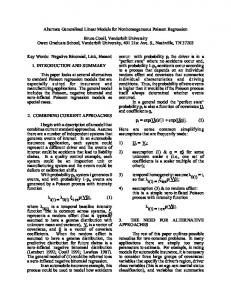
We begin with a toy example that shows how inference based on the Poisson Transform can be implemented in the non-IID case, and show that semiparametric inference using non-contrastive divergence can be almost as efficient as maximum-likelihood (and much more efficient than completely parametric non-contrastive divergence). In addition, we will see that ignoring normalisation constants as done by Mnih and Teh (2012b) and Mnih and Kavukcuoglu (2013) can lead to severe bias. We have made available a detailed companion document for this section, which includes all the code necessary to replicate our results in R. Our toy example is a Markov chain in [−1, 1], with transition probability:   1 2 (4.1) pθ (yt |yt−1 ) ∝ exp θ1 yt − θ2 (yt − yt−1 ) I[−1,1] (yt ). 2 We picked this example because it is a simplified version of the spatial

4.1 A toy example

0.0 −1.0

−0.5

yt

0.5

1.0

11

0

20

40

60

80

100

Time

Fig. 4.1: Two realisations from the toy model, a Markov chain constrained to the interval [−1, 1] (eq. 4.1). Red, unfilled dots: θ1 = 0, θ2 = 2. Blue, solid dots: θ1 = −2, θ2 = 10. As expected, the second chain shows a bias towards negative values as well as stronger autocorrelation. Markov chains we study in the following section. Two realisations from the chain are shown on Fig. 4.1. In this one-dimensional example it is of course easy to compute the normalisation constant using numerical integration, and thus maximum likelihood inference is possible. To use non-constrastive divergence, we need to pick a reference kernel, and here a uniform, IID distribution does the job quite well: q(y|yt−1 ) = 21 I[−1,1] (y). Positive examples for the logistic regression are formed from actual pairs (yt , yt−1 ), negative examples are formed from pairs (rit , yt−1 ), i = 1, . . . , k, i.e. one replaces the actual value of yt with k uniform variates. Thus, there are k reference points per datapoint: m = kn. We note (ut , ut−1 ) a generic point (either true data, or reference data). The log-odds for the semi-parametric logistic regression are then, injecting (4.1) into (3.4): 1 mθ (ut ) = θ1 ut − θ2 (ut − ut−1 )2 + χ(ut−1 ) + log(n/m) − log (1/2) , 2 = θ1 ut + θ2 dt + χ(ut−1 ) + cst. (4.2) where dt = 21 (ut − ut−1 )2 . From a practical perspective, the logistic regression can be performed with ut and dt entering as linear effects, and χ(ut−1 ) as a smooth, nonlinear effect. The constant term may be added as an offset for completeness. (It makes no practical difference since it can be absorbed into χ (ut−1 ) or the intercept. One needs to include it only if intercepts are penalised.). The completely parametric variant of (4.2) corresponds to having a different intercept for every value of ut−1 . Alternatively, neglecting the normalisation

12

4 Applications to spatial Markov chains

constants means replacing χ(ut−1 ) with an intercept term (or, put another way, forcing χ (ut−1 ) to be constant). Semiparametric inference can be performed using R package mgcv (Wood, 2006). To measure the efficiency of the various estimation methods, we simulated realisations of the chain at a fixed parameter setting of θ1 = −2, θ2 = 50 for increasing n. We also used two different values of k (the ratio of reference points to real data), k = 10 and k = 30. On each simulation we picked two parameter 1 values at random: θ1 ∼ U(−1, 1), θ2 ∼ U( 10 , 10), generated n datapoints, and obtained the 4 different estimates. We used 300 repetitions for each value of n and k. Results are shown on Fig. 4.2. Semiparametric inference performs almost as well as ML. Fully parametric inference is much more variable, although it becomes better for larger values of k. Indeed, theory predicts that it for large enough k it becomes equivalent to ML. The variant of non-contrastive divergence which neglects the normalisation constants performs quite well for θ2 but shows asymptotic bias in θ1 . The bias comes from the missing non-linear effect χ (ut−1 ), which is projected on the linear effect for ut . This happens because the two are correlated through the dependencies in the chain. Neglecting the normalisation constants then effectively leads to confounding. Contrary to the ideal Poisson transform (see correlary 6), the non-contrastive divergence approximation is noisy and it is possible to overfit the nonparametric term χ (ut−1 ). Cross-validation is a valid way of selecting the penalisation level, and here in practice related criteria such as Generalised Cross-Validation and REML work just as well. The results in Fig. 4.2 are obtained using the default criterion (GCV).

4.2

Spatial Markov chains for eye movement data

A perennial problem in spatial statistics is to predict where certain events are likely to take place (for example, cases of malaria in a country) given past occurences and a set of spatial predictors (for example, availability of mosquito nets). Point process models can be used in such contexts, and one important class of applications is to eye movement data (Barthelmé et al., 2013), where the goal is to predict which locations people will look at in a given visual stimulus (for example a photograph). Eye movements are reliably drawn to certain features in a stimulus, but also exhibit dependencies (Engbert et al., 2014), and the most important of these is that we tend not to move our eyes very much. If we are currently fixating on the bottom-left corner of the screen, it will take a few steps for us to go look in the upper right, even if there is something rather interesting there. The presence of dependencies motivates the introduction of models of eye movements as spatial Markov chains. Here we note yt the fixation location at time t, and use a log-linear form for the kernel: p (yt |yt−1 ) ∝ exp {s (yt ) + r (yt , yt−1 )}

(4.3)

4.2 Spatial Markov chains for eye movement data

13

Fig. 4.2: Estimation errors of ML vs three variants of NCD for the onedimensional Markov chain. The variants are: fully parametric (one νi term per datapoint), semi-parametric (normalisation constants are modelled as a smooth function), ignoring constants (logistic regression with a single intercept, as in Mnih and Teh, 2012a). The semiparametric estimate is almost as good as the ML estimate across the board. The fully parametric estimate performs very poorly when there are few reference points per datapoint (compare the red line across the left and right panels). Finally, neglecting normalisation constants leads to an non-convergent estimator of θ1 , although performance on θ2 is very good. See the companion document for a more thorough discussion of this phenomenon.

14

4 Applications to spatial Markov chains

Fig. 4.3: A sequence of eye movements extracted from the dataset of Kienzle et al. (2009). Fixation locations are in red and successive locations are linked by a straight line. where s(yt ) represents purely spatial factors, and r (yt , yt−1 ) is an interaction term that represents spatial dependencies. A well-known factor affecting fixation locations is the centrality bias (Tatler and Vincent, 2009), a preference for looking at central locations, and we take s(yt ) to be a smooth function of ||yt || (the distance to the center): s(yt ) = s(kyt k). Potential interactions between successive locations include a tendency not to stray too far from the current location (Engbert et al., 2014), and a tendency for making movements along the cardinal axes (vertical and horizontal, Foulsham et al., 2008). We therefore further decompose r (yt , yt−1 ) into r (yt , yt−1 ) = rdist (||yt − yt−1 ||) + rang (∠ (yt − yt−1 ))

(4.4)

the sum of a distance and an angular component. We model the unknown functions s, rdist and rang non-parametrically, using smoothing splines. The corresponding estimators are therefore obtained by penalised likelihood maximisation, and the Poisson transform extends straightforwardly to this case: replace the maximisation of L(θ) − pen(θ) by the maximisation of M(θ, χ) − pen(θ), where θ = (s, rdist , rang ), and χ is a non-parametric function used to estimate the normalising constant, as explained in the previous section. We use the data of Kienzle et al. (2009), who recorded eye movements while subjects where exploring a set of photographs (Fig. 4.3). There are 14 subjects, each contributing between 600 and 2,000 datapoints. Thanks to the techniques described above, the model described by (4.3) can be turned into a logistic regression, and the R package mgcv (Wood, 2006) can be used to estimate the different components using smoothing splines. We used a uniform, IID refer−1 ence kernel q(yt |yt−1 ) = |Ω| to produce negative examples, with 20 times as many negative examples as positive. Although the logistic approximation introduces Monte Carlo variance, the estimates are very stable (see Appendix). We fit separate functions for each subject to account for interindividual variability. The results are shown on Fig. 4.4. We replicate known effects from the literature: central locations dominate (although some subjects may display an

15

0 1.0

Estimated effect

0

−2

0.5

−1 0.0 −4

−0.5

−2

−6 −1.0 −π

−π 2

0

π 2

Saccade angle (rel. to vertical)

π

0

100

200

300

400

Distance to previous fixation (pix.)

500

0

100

200

300

400

500

Distance to center (pix.)

Fig. 4.4: Eye movement model. The smooth terms in eq. 4.3 and 4.4 are estimated using smoothing splines by reducing the model to a nonparametric logistic regression. The different panels display the estimated effects of saccade angle (rang ), distance to previous fixation (rdist ) and centrality bias (s). Individual subjects are in gray, and the group average is in blue.

off-center bias), and dependencies include both a inhibitory effect of distance and a preference for movements along cardinal orientations. Once the data have been put into a suitable format, model fitting can be performed in one line of R code (see Appendix) and takes around 5 minutes on a normal desktop. The Poisson transform thus turns an otherwise highly non-standard model into a convenient Generalised Additive Model.

5

Discussion

The Poisson transform suggests a new way of thinking about inference in unnormalised models: if we think of the data as coming from a point process, the integration constant becomes just another parameter to estimate. We have shown that the same idea extends to unnormalised models in the sequential context and in the presence of covariates, in which case parametric estimation may be turned into a semi-parametric problem. Practical approximations of Poissontransformed likelihoods can be computed using Monte Carlo or using logistic likelihoods that follow from a reinterpretation of noise-contrastive divergence. Part of the challenge in applying the Poisson transform to models with highdimensional covariates or dependencies on a high-dimensional vector of past values will be in the design of appropriate kernels for the non-parametric part, which corresponds to conditional normalisation constants. The great advantage of the reduction to logistic regression is that we will be able to leverage the existing literature on nonlinear classification and dimensionality reduction, including recent developments in hashing (Li and König, 2011). Inference in unnormalised models will probably always remain challenging, but we believe the Poisson transform should alleviate some of the difficulties.

A Derivatives of Poisson-transformed likelihoods

16

A

Derivatives of Poisson-transformed likelihoods

The first and second derivatives of L (θ) and M (θ, ν) are needed in the proofs and we collect them here. Derivatives of L (θ):

L(θ)

=

n X

ˆ fθ (yi ) − n log

 n X exp {fθ (s)} ds := fθ (yi ) − nφ (θ)

i=1

i=1

ˆ

  ∂ ∂ fθ (s)exp {fθ (s) − φ (θ)} ds = Eθ fθ ∂θ ∂θ  2    t !  t   ∂ ∂ ∂ ∂ ∂ Eθ fθ + Eθ fθ fθ fθ Eθ fθ − Eθ ∂θ 2 ∂θ ∂θ ∂θ ∂θ

∂ φ (θ) ∂θ

=

∂2 φ (θ) ∂θ 2

=

∂ L ∂θ

=

n X ∂ d fθ (yi ) − n φ (θ) ∂θ dθ i=1

∂2 L (θ) ∂θ 2

=

X ∂2 d2 f (y ) − n φ (θ) θ i ∂θ 2 dθ 2

where we have used Eθ as shorthand for the expectation with respect to density exp {fθ (s) − φ (θ)}. Derivatives of M (θ, ν):

M (θ, ν)

=

∂ M (θ, ν) ∂θ

=

∂ M (θ, ν) ∂ν

=

∂2 M (θ, ν) ∂θ 2

=

∂2 M (θ, ν) = ∂ν 2 ∂ M (θ, ν) = ∂θ∂ν

n X

ˆ {fθ (yi ) + ν} − n

exp {fθ (s) + ν} ds

i=1 n X

  ∂ ∂ fθ (yi ) − nEθ,ν fθ ∂θ ∂θ i=1 ˆ n − n exp {fθ (s) + ν} ds

 2  X ∂2 ∂ f (y ) − n E fθ + Eθ,ν θ i θ,ν ∂θ 2 ∂2θ ˆ −n exp {fθ (s) + ν} ds   ∂ −nEθ,ν fθ ∂θ



∂ fθ ∂θ

where we have used Eθ,ν as shorthand for the linear operator Eθ,ν (ϕ) = (which is not an expectation in general).

´



∂ fθ ∂θ

t !!

ϕ(s)exp {fθ (s) + ν} ds

17

B

Further properties of the Poisson transform

B.1

The Poisson transform preserves confidence intervals

The usual method for obtaining confidence intervals for θ is to invert the Hessian matrix of L (θ) at the mode, θ ? :  CL =

−

d2 L |θ=θ? d2 θ

−1

We can show that the same confidence intervals can be obtained from M (θ, ν) at the joint mode, θ ? , ν ? . At the joint maximum, ν ? normalises the intensity function, and the Hessian of M equals: #  " ∂2 ∂ M (θ, ν) M (θ, ν) Haa Hba ∂2θ ∂θ∂ν = = ∂ ∂2 Hab Hbb M (θ, ν) ∂ν∂θ ∂ 2 ν M (θ, ν)  2   " P 2
∂
t 
t # ∂ ∂ ∂ ∂ −nE f (y ) − nE f − nE f f f 2 2 θ θ i θ θ θ θ θ ∂θ ∂ θ ∂θ ∂θ ∂θ =
∂ −nEθ ∂θ fθ −n 

H

where again E denotes the expectation with respect to density exp {fθ (s) − φ (θ)}. Inverting −H also yields confidence intervals. By the inversion rule for block matrices, the approximate covariance for θ using M (θ, ν) equals C−1 M


= − Haa − Hba H−1 bb Hab   t !  1 2 ∂ ∂ = − Haa + n Eθ fθ Eθ fθ n ∂θ ∂θ "  2  X ∂2 ∂ f (y ) − nE f = − θ i θ ∂θ 2 ∂2θ   t !    t # ∂ ∂ ∂ ∂ −nEθ fθ fθ fθ E fθ + nEθ ∂θ ∂θ ∂θ ∂θ = C−1 L

B.2

Preservation of log-concavity in exponential families

In exponential families, the log-likelihood is concave, which facilitates inference. The Poisson transform preserves this log-concavity. In the natural parameterisation, exponential-family models are given by: ( n ) X L (θ) = exp s(yi )t θ − φ (θ) i=1

B Further properties of the Poisson transform

18

with s(y) a vector of sufficient statistics. The second derivative of L (θ) simplifies to: ˆ
1 ∂ − L (θ) = s(y)s(y)t exp s(y)t θ − φ (θ) 2 n∂ θ  = Eθ s(y)s(y)t a p.s.d. matrix, which establishes concavity. The second derivatives of M (θ, ν) (Section A) also simplify ˆ
1 ∂2 ? − M (θ, ν) = exp {ν − ν (θ)} s(y)s(y)t exp s(y)t θ − φ (θ) n ∂θ 2 ˆ
1 ∂2 ? − M (θ, ν) = exp {ν − ν (θ)} s(y) exp s(y)t θ − φ (θ) n ∂ν∂θ 1 ∂2 M (θ, ν) = exp {ν − ν ? (θ)} − n ∂ν 2 so that the full Hessian H can be written in block-form as: o n t E s (y) s (y) θ 1 n o − exp {ν ? (θ) − ν} H =  t n Eθ s (y) 

E (s (y))

 =A

1

and H is n.s.d if and only if for all x, c such that (x, c) 6= 0:    t  x x c A >0 c which the following establishes: 

n o   t Eθ s (y) s (y) E {s (y)} n o  xt c  t Eθ s (y) 1  n o t   Eθ s (y) s (y) x + cEθ {s (y)} n o = xt c  t Eθ s (y) x + c n o  t =Eθ xt s (y) s (y) x + 2Eθ xt s (y) c + c2  2  t =Eθ s (y) x + c >0 



x c 





assuming Eθ {s(y)s(y)t } is p.s.d. for all θ.

B.3

Noise-constrative divergence approximates the Poisson transform (Theorem 7)

We have assumed that

B.3 Noise-constrative divergence approximates the Poisson transform (Theorem 7)

19

fθ (y) − log q(y) ≤ C(θ) for a certain constant C(θ) that may depend on θ, and all y ∈ Ω. We rewrite the log-odds ratio as h(y) − log(m) where h(y) := fθ (y) + ν − log q(y) + log(n) ¯ := C(θ) + ν + log(n). One has: does not depend on m; note h(y) ≤ h   n X m exp {fθ (yi ) + ν} m R (θ, ν) + log(m/n) = log n exp {fθ (yi ) + ν} + mq(yi ) i=1   m X mq(rj ) + log n exp {fθ (rj ) + ν} + mq(rj ) j=1 where the first term trivially converges (as m → +∞) to n X

{fθ (yi ) + ν − log q(yi )} .

i=1

Regarding the second term, one has:     mq(rj ) 1 = log 1 − log n exp {fθ (rj ) + ν} + mq(rj ) 1 + m exp {−h(rj )} where 0≤

1 1 ¯ ≤ exp(h). 1 + m exp {−h(rj )} m

Since |log(1 − x) + x| ≤ x2 for x ∈ [0, 1/2], we have, for m large enough, that   ¯ exp(2h) mq(rj ) 1 log ≤ + (B.1) n exp {fθ (rj ) + ν} + mq(rj ) 1 + m exp {−h(rj )} m2 and

¯ exp(2h) 1 1 − exp {h(r )} j ≤ 1 + m exp {−h(rj )} m 2 m

and since, by the law of large numbers, m

1 X exp {h(ri )} → Eq [exp {h(ri )}] = n m j=1

ˆ exp {fθ (y) + ν} dy < +∞ (B.2)

almost surely as m → +∞, one also has:   ˆ m X mq(yi ) log → −n exp {fθ (y) + ν} dy n exp {fθ (yi ) + η} + mq(yi ) j=1 almost surely, since the difference between the two sums is bounded determin¯ istically by exp(2h)/m.

B Further properties of the Poisson transform

20

B.4

Uniform convergence of the noise-constrative divergence (Theorem 8)

We first prove two intermediate results. Lemma 9. Assuming that |fθ (y) − log q(y)| ≤ C for all y ∈ Ω, then there exists a bounded interval I such that, for any θ, the maximum of both functions ν → M(θ, ν) and ν → Rm (θ, ν) is attained in I. ´ Proof. Let θ some fixed value. M(θ, ν) is maximised at ν ? (θ) = − log Ω exp {fθ (y)} dy ∈ [−C, C], since e−C q ≤ fθ ≤ eC q. For Rm (θ, ν), using again e−C q ≤ fθ ≤ eC q, one sees that l(ν) ≤ Rm (θ, ν) ≤ u(ν), where l and u are functions of ν that diverges at −∞ for both ν → +∞ and ν → −∞; i.e.   n X m exp {C + ν} m log R (θ, ν) + log(m/n) ≤ u(ν) := n exp(−C + ν) + m i=1   m X m log + n exp {−C + ν} + m j=1 and the lower bound l(ν) has a similar expression. Thus one may construct an interval J such that the maximum of function ν → Rm (θ, ν) is attained in J for all θ (e.g. take J such that for ν ∈ J c , u(ν) ≤ Ml /2, l(ν) ≤ Ml /2, with Ml = supν l) . To conclude, take I = J ∪ [−C, C]. We now establish uniform convergence, but, in light of the previous result, we restrict ν to the interval I defined in Lemma 9. Lemma 10. Under the Assumptions that (i) Θ is bounded, that (ii) |fθ (y) − log q(y)| ≤ C for all y ∈ Ω, that (iii) |fθ (y) − fθ0 (y)| ≤ κ(y) kθ − θ 0 k with κ such that Eq [κ] < ∞, one has, for fixed S = {y1 , . . . , yn }: n X m sup R (θ, ν) + log(m/n) + log q(yi ) − M(θ, ν) → 0 (B.3) (θ,ν)∈Θ×I i=1

almost surely, relative to the randomness induced by R = {r1 , . . . , rm } . Proof. Recall that the absolute difference above was bounded by the sum of three terms in the previous Appendix. The first term was    n  X m exp {fθ (yi ) + ν} log − {fθ (yi ) + ν − log q(yi )} n exp {fθ (yi ) + ν} + mq(yi ) i=1 which clearly converges deterministically to 0 as m → +∞. In addition, this convergence is uniform with respect to (θ, ν) ∈ Θ × I, since |log x − log y| ≤ c |x − y| for x, y ≥ 1/c, and here, by Assumption (ii), x :=

m exp {fθ (yi ) + ν} m exp {−C + ν} ≥ ≥ exp {−C + ν} n exp {fθ (yi ) + ν} + mq(yi ) n exp {C + ν} + m

21

and y = exp {fθ (yi ) + ν − log q(yi )} ≥ exp {−C + ν}, so both x and y are lower bounded since ν ∈ I. Similarly (x − y) is bounded by C 0 /m, where C 0 is some constant independent of θ. 2 ¯ ¯ an upper The second term, see (B.1), was bounded by exp(2h)/m , where h, bound of h, may now be replaced by a constant, since h(y) := fθ (y) + ν − log q(y) + log(n) ≤ C + ν + log(n) and ν ∈ I, again by Assumption (ii). The third term is related to the law of large numbers (B.2) for random variable H(θ,η) (ri ) := exp {h(ri )}, which depended implicitly on (θ, η): H(θ,η) (ri ) =

n exp {fθ (ri ) + ν} . q(ri )

To obtain (almost surely) uniform convergence, we use the generalised version of the Glivenko-Cantelli theorem; e.g. Theorem 19.4 p.270 in Van der Vaart (2007). From Example 19.7 of the same book, one sees that a sufficient condition in our case is that Θ is bounded (Assumption (i)), and that H(θ,η) (r) − H(θ0 ,η0 ) (r) ≤ m(r) kξ − ξ 0 k for ξ = (θ, η), ξ 0 = (θ 0 , η 0 ), and m a function such that Eq [m] < ∞. But H(θ,η) (r) − H(θ0 ,η0 ) (r) = n exp {fθ (r) + ν} |1 − exp {fθ (r) + ν − fθ0 (r) − ν 0 }| q(r) ≤ neC+ν |1 − exp {fθ (r) + ν − fθ0 (r) − ν 0 }| ≤ C 0 {κ(r) kθ − θ 0 k + |ν − ν 0 |} ≤ C 0 {κ(r) + 1} kξ − ξ 0 k by Assumption (ii), and for some constant C 0 independent of θ, since |1 − ex | ≤ Kx for x, y in a bounded set. One may conclude, since, by Assumption (ii), Eq [κ] < ∞. We are now able to prove Theorem 8. Again, let ξ = (θ, ν), and rewrite any function of (θ, ν) as a function of ξ, i.e. M(ξ), Rm (ξ). By e.g. Theorem 5.7 p.45 of Van der Vaart (2007), the uniform convergence B.3 implies that that the maximiser ξˆm of Rm (θ, ν) converges to the maximiser ξˆ of M(θ, ν), provided that (a) the maximisation is with respect to (θ, ν) ∈ Θ × I; and (b) ˆ However, by Lemma 9 one sees that in (a) that supd(ξ,ξ)≥ M(ξ) < M(ξ). ˆ the same estimators would be obtained by maximising instead with respect to (θ, ν) ∈ Θ × R, and (b) is a direct consequence of Assumption (iv) of the ˆ the supremum norm of ξ − ξ. ˆ theorem, if one takes for d(ξ, ξ)

C

Additional information on the application

In our application we fit a spatial Markov chain model using logistic regression. Since the procedure involves the generation of a random set of reference points, we incur some Monte Carlo error in the estimates. Estimating the magnitude of

C Additional information on the application

22

Subject 1

Subject 2

Subject 3

Subject 4

Subject 5

Subject 6

Subject 7

Subject 8

Subject 9

Subject 10

Subject 11

Subject 12

Subject 13

Subject 14

1

0

−1

1

Estimated effect

0

−1

1

0

−1

1

0

−1

−2

0

2

−2

0

2

Saccade angle (rel. to vertical)

Fig. C.1: Eye movement model: 5 independent replications of the estimates under different sets of random reference points. We show here the estimated effect of saccade angle with an associated 95% pointwise confidence interval. The 5 replicates are in different colours and overlap each other almost completely, showing that 20 reference points per true datapoint are more than enough to produce stable estimates.

the Monte Carlo error is just a matter of running the procedure several times to look at variability in the estimates. We did so over 5 repetitions and report the results in Fig. C.1. For each repetition we plot the estimated smooth effect of saccade angle rang , along with a 95% confidence band. Since smoothing splines are used, smoothing hyperparameters had to be inferred from the data (using REML, Wood, 2011), and the reported confidence band is conditional on the estimated value of the smoothing hyperparameters. The fits and confidence bands are extremely stable over independent repetitions. The R command we used was: gam(class ~ s(delta,k=10)+s(dcenter,k=40)+s(fxc.prev,fyc.prev,k=40) +s(angle,bs="cc",k=20),data=data,family=binomial,method=”REML”)

REFERENCES

23

References Baddeley, A., Berman, M., Fisher, N. I., Hardegen, A., Milne, R. K., Schuhmacher, D., Shah, R., and Turner, R. (2010). Spatial logistic regression and change-of-support in poisson point processes. Electronic Journal of Statistics, 4(0):1151–1201. Baddeley, A., Coeurjolly, J.-F., Rubak, E., and Waagepetersen, R. (2014). Logistic regression for spatial gibbs point processes. Biometrika, page ast060. Baker, S. G. (1994). The Multinomial-Poisson transformation. Journal of the Royal Statistical Society. Series D (The Statistician), 43(4):495–504. Barthelmé, S., Trukenbrod, H., Engbert, R., and Wichmann, F. (2013). Modeling fixation locations using spatial point processes. Journal of vision, 13(12). Bengio, Y. and Delalleau, O. (2009). Justifying and generalizing contrastive divergence. Neural computation, 21(6):1601–1621. Caimo, A. and Friel, N. (2011). Bayesian inference for exponential random graph models. Social Networks, 33(1):41–55. Engbert, R., Trukenbrod, H. A., Barthelmé, S., and Wichmann, F. A. (2014). Spatial statistics and attentional dynamics in scene viewing. Foulsham, T., Kingstone, A., and Underwood, G. (2008). Turning the world around: Patterns in saccade direction vary with picture orientation. Vision Research, 48(17):1777–1790. Geyer, C. J. (1994). Estimating normalizing constants and reweighting mixtures in markov chain monte carlo. Technical Report 568, School of Statistics, University of Minnesota. Girolami, M., Lyne, A.-M., Strathmann, H., Simpson, D., and Atchade, Y. (2013). Playing russian roulette with intractable likelihoods. arxiv 1306.4032. Gu, M. G. and Zhu, H.-T. (2001). Maximum likelihood estimation for spatial models by markov chain monte carlo stochastic approximation. Journal of the Royal Statistical Society: Series B (Statistical Methodology), 63(2):339–355. Gutmann, M. and ichiro Hirayama, J. (2011). Bregman divergence as general framework to estimate unnormalized statistical models. In Cozman, F. G. and Pfeffer, A., editors, UAI, pages 283–290. AUAI Press. Gutmann, M. U. and Hyvärinen, A. (2012). Noise-contrastive estimation of unnormalized statistical models, with applications to natural image statistics. J. Mach. Learn. Res., 13(1):307–361. Hastie, T., Tibshirani, R., and Friedman, J. H. (2003). The Elements of Statistical Learning. Springer, corrected edition.

24

REFERENCES

Hinton, G. E. (2002). Training products of experts by minimizing contrastive divergence. Neural Comput., 14(8):1771–1800. Kienzle, W., Franz, M. O., Schölkopf, B., and Wichmann, F. A. (2009). Centersurround patterns emerge as optimal predictors for human saccade targets. Journal of vision, 9(5). Kingman, J. F. C. (1993). Poisson Processes (Oxford Studies in Probability). Oxford University Press. Li, P. and König, A. C. (2011). Theory and applications of b-bit minwise hashing. Commun. ACM, 54(8):101–109. Minka, T. (2005). Divergence Measures and Message Passing. Technical report, Microsoft Research Technical Report. Mnih, A. and Kavukcuoglu, K. (2013). Learning word embeddings efficiently with noise-contrastive estimation. In Burges, C., Bottou, L., Welling, M., Ghahramani, Z., and Weinberger, K., editors, Advances in Neural Information Processing Systems 26, pages 2265–2273. Curran Associates, Inc. Mnih, A. and Teh, Y. W. (2012a). A fast and simple algorithm for training neural probabilistic language models. In Proceedings of the 29th International Conference on Machine Learning, pages 1751–1758. Mnih, A. and Teh, Y. W. (2012b). A fast and simple algorithm for training neural probabilistic language models. In Proceedings of the 29th International Conference on Machine Learning, ICML 2012, Edinburgh, Scotland, UK, June 26 - July 1, 2012. Møller, J., Pettitt, A. N., Reeves, R., and Berthelsen, K. K. (2006). An efficient Markov chain Monte Carlo method for distributions with intractable normalising constants. Biometrika, 93(2):451–458. Murray, I., Ghahramani, Z., and MacKay, D. (2012). intractable distributions.

MCMC for doubly-

Pihlaja, M., Gutmann, M., and Hyvärinen, A. (2010). A family of computationally E cient and simple estimators for unnormalized statistical models. In UAI 2010, Proceedings of the Twenty-Sixth Conference on Uncertainty in Artificial Intelligence, Catalina Island, CA, USA, July 8-11, 2010, pages 442–449. Salakhutdinov, R. and Hinton, G. E. (2009). Deep boltzmann machines. In International Conference on Artificial Intelligence and Statistics, pages 448– 455. Schölkopf, B. and Smola, A. J. (2001). Learning with kernels : support vector machines, regularization, optimization, and beyond. The MIT Press, 1st edition.

REFERENCES

25

Tatler, B. and Vincent, B. (2009). The prominence of behavioural biases in eye guidance. Visual Cognition, 17(6):1029–1054. Van der Vaart, A. W. (2007). Asymptotic Statistics. Cambrige series in statistical and probabilistic mathematics. Walker, S. G. (2011). Posterior sampling when the normalizing constant is unknown. Communications in Statistics - Simulation and Computation, 40(5):784–792. Wang, C., Komodakis, N., and Paragios, N. (2013). Markov random field modeling, inference & learning in computer vision & image understanding: A survey. Computer Vision and Image Understanding, 117(11):1610–1627. Welling, M. and Teh, Y. W. (2011). Bayesian learning via stochastic gradient Langevin dynamics. In Proceedings of the 28th International Conference on Machine Learning (ICML-11), pages 681–688. Wood, S. (2006). Generalized Additive Models: An Introduction with R (Chapman & Hall/CRC Texts in Statistical Science). Chapman and Hall/CRC, 1 edition. Wood, S. N. (2011). Fast stable restricted maximum likelihood and marginal likelihood estimation of semiparametric generalized linear models. Journal of the Royal Statistical Society: Series B (Statistical Methodology), 73(1):3–36.