9, SEPTEMBER 2012. 2501. Three-Axial Accelerometer Calibration Using. Kalman Filter Covariance Matrix for Online. Estimation of Optimal Sensor Orientation.
IEEE TRANSACTIONS ON INSTRUMENTATION AND MEASUREMENT, VOL. 61, NO. 9, SEPTEMBER 2012
2501
Three-Axial Accelerometer Calibration Using Kalman Filter Covariance Matrix for Online Estimation of Optimal Sensor Orientation Tadej Beravs, Janez Podobnik, and Marko Munih, Member, IEEE
Abstract—Inexpensive inertial/magnetic measurement units can be found in numerous applications and are typically used to determine orientation. Due to the presence of nonidealities in measurement systems, the calibration of the sensor is thus needed to determine sensor parameters such as bias, misalignment, and gain/sensitivity. In this paper, an online automatic calibration method for a three-axial accelerometer is presented. Parameters are estimated using an unscented Kalman filter. The sensor is placed in a number of different orientations using a robotic arm. These orientations are calculated online from the parameter covariance matrix and represent estimated optimal sensor orientations for parameter estimation. Numerous simulations are run to evaluate the proposed calibration method, and a comparison is made with an offline least mean squares calibration method. The simulation results show that calibration with the proposed method results in higher accuracy of parameter estimation when using less than 100 iterations. The proposed calibration method is also applied to a real accelerometer using a low number of iterations. The results show only slight (less than 0.4%) changes in parameter values between different calibration runs. The proposed calibration method provides an accurate parameter estimation using a small number of iterations without the need for manually predefining orientations of the sensor, and the method can be used in combination with other offline calibration methods to achieve even higher accuracy. Index Terms—Accelerometer calibration, orientation determination, sensor parameter estimation, unscented Kalman filtering (UKF).
I. I NTRODUCTION
M
ICROELECTROMECHANICAL inertial measurement units (IMUs) are inexpensive lightweight sensors that are used for orientation estimation in numerous applications. They can be found in inertial navigation systems [1], [2], robotics [3], the automotive industry, analysis of daily activities
Manuscript received September 20, 2011; revised December 9, 2011; accepted December 11, 2011. Date of publication March 5, 2012; date of current version August 10, 2012. This work was supported in part by the European Union through the EVRYON Collaborative Project STREP under Grant FP7-ICT-2007-3-231451 and by the Slovenian Research Agency. The Associate Editor coordinating the review process for this paper was Dr. Subhas Mukhopadhyay. The authors are with the Laboratory of Robotics, Department of Measurement and Robotics, Faculty of Electrical Engineering, University of Ljubljana, 1000 Ljubljana, Slovenia. Color versions of one or more of the figures in this paper are available online at http://ieeexplore.ieee.org. Digital Object Identifier 10.1109/TIM.2012.2187360
[4], and measurement of human body kinematics [5], where IMUs can replace optical measurement systems, which measure body part orientations. [6]. Consisting of accelerometers, gyroscopes, and (optionally) magnetometers, IMUs can achieve good dynamic specifications with a relatively low investment. Several IMUs are commercially available; however, custom developed IMUs have some advantages such us small size, which allows integration in various applications, custom wireless connectivity, and open architecture, which allows different modifications and implementations of algorithms. However, similar to any measurement systems, IMUs also suffer from numerous disadvantages such as sensor misalignment, large offset, nonlinearity, drift, and random noise. These disadvantages are generally addressed using sensor calibration. Several offline calibration methods exist. One simple method proposes the calibration of two main parameters with manual sensor movement in six different orientations with a relatively simple mathematical algorithm (the sum of output signals is equal to the gravity vector) [7]. Similar approaches that demand several different sensor orientations are described in [8], where all three parameters are determined through the Levenberg–Marquardt algorithm, similar to [9], where the parameters are determined using the Newton iterative arithmetic. More sophisticated methods are described in [10], where sensor parameters are estimated using optical alignment and a least mean squares algorithm, and in [11], the reference orientation of the sensor is also included in determining the sensor parameters. One method where the robot arm is used to position the sensor to a known predefined orientation is presented in [12], where the parameters of the sensor (including the alignment angle of the robot in the gravitational field and the alignment between the sensor and robot end effector) are again determined using least mean squares methods. However, because several of the factors that contribute to sensor errors are time varying (e.g., temperature), initial offline calibration cannot completely negate their effects. Thus, an online calibration procedure could potentially achieve higher accuracy. Compared with offline calibration, where parameters are estimated using different mathematical algorithms after obtaining all measurements from the sensor, the online calibration estimates parameters during each iteration, and after the last iteration, the estimation of parameters is completed. Online approaches have been demonstrated in [13] and [14] using sophisticated hardware, but the different sensor orientations needed for the calibration must be predefined in both cases. An appropriate orientation must be chosen, or a large number
0018-9456/$31.00 © 2012 IEEE
2502
IEEE TRANSACTIONS ON INSTRUMENTATION AND MEASUREMENT, VOL. 61, NO. 9, SEPTEMBER 2012
of random orientations must be determined to accomplish an accurate calibration. In this paper, we present an automatic calibration method of the accelerometer, where parameters and orientations are estimated by an unscented Kalman filter (UKF), and a robotic arm is used to place the sensor in the calculated orientation. Unlike [12], where the sensor is placed in a large number of manually predefined orientations using a robotic arm and the parameters are calculated offline, our proposed method uses online parameter estimation without the need for predefined orientations, because they are calculated and used during calibration. The method described in [13] uses online parameter estimation; however, the orientations of the sensor must be predefined. The method is used to determine all three main parameters (gain, misalignment, and bias) together with the alignment angles of the robot in the gravitational field and alignment angles between the sensor and robot end effector (because the flange and sensor board are not perfectly aligned). The proposed method repeatedly uses the covariance matrix decomposition for estimation of maximal sensitivity axis (CEMS) to estimate the next orientation in which the sensor should be placed for optimal parameter estimation. This condition causes fast method convergence. The sensor is thus placed in a small number of automatically determined orientations, eliminating the need for a large number of predefined orientations and, this way, allowing faster calibration compared to methods where sensor orientations must be predefined and the manipulation of the sensor is manually done. Because the sensor is placed in orientations that allow the most effective parameter estimation and all the data can be recorded, offline methods can also be applied later for parameter estimation. The CEMS calibration approach can be applied for the accelerometer or the magnetometer. The only difference between the two sensors is in the initial description of the gravitational and magnetic fields. However, the magnetic field is very sensitive to environmental noise, and a homogenous magnetic field is needed for successful calibration. The CEMS calibration method is thus applied here only to the accelerometer, because the magnetic field that surrounds the robot arm is not homogenous. This paper is organized as follows. The developed wireless IMU system and the corresponding mathematical model of the sensor system in conjunction with the robot arm are described in the first part of Section II. Parameter estimation with UKF is described together with the method for determining the sensor orientation using singular value decomposition (SVD) in the second part of Section II. The simulation and measurement procedures are described at the end of the section. Simulation and measurement results are presented in Section III, and a detailed discussion is given in Section IV. Section V summarizes the proposed calibration method and the contributions of this paper.
II. M ETHODS A. Hardware Design 1) IMU: The IMU consists of the following three digital sensors: 1) an Invensense three-axis gyroscope; 2) an STmicro-
Fig. 1. IMU that consists of a three-axis gyroscope, a three-axis magnetometer, and a three-axis accelerometer and a wireless module with a dual-chip antenna. The size of the IMU is 30 × 20 × 5 mm without a battery.
electronics three-axis accelerometer; and 3) a Honeywell threeaxis magnetometer. The gyroscope has selectable full-scale ranges of ±250◦ /s, ±500◦ /s, ±1000◦ /s, and ±2000◦ /s and software-selectable low-pass filters. Each axis is represented with 16 b. The gyroscope also measures temperature for additional software compensation. The sampling rate of the gyroscope is 1000 Hz. Similar to the gyroscope, the accelerometer also offers a selectable range of ±2, ±4, and ±8 g and has 16-b output per axis. It offers software selection of high-pass filters and sampling rates. The highest possible sampling rate of the accelerometer is 1000 Hz. The magnetometer has a selectable range of ±0.88–±8.1 G. It uses an internal 12-b analog-todigital converter and has a significantly lower sampling rate compared with the other two sensors. The sampling rate of the magnetometer can be selected from 0.75 Hz to 160 Hz. Thus, the maximum sampling rate of the IMU system is 160 Hz when data from all three sensors, including the magnetometer, are simultaneously acquired. All sensors are connected to an interintegrated circuit (I2C) bus with a maximum data transfer rate of 222 kb/s. Each sensor provides 6 B of information (2 B per axis), for a total of 18 B. The theoretically attainable data transfer rate of the I2C communication protocol is 1.2 kHz, but the maximum data transfer rate is set to 300 Hz due to limitations of the wireless transceiver module that provides the connection to the central unit. The IMU itself (without battery) has a size of 30 × 20 × 5 mm and is shown in Fig. 1. The battery is placed away from the IMU to avoid interference with the magnetometer. 2) Data Transmission and Central Unit: The IMU is connected to a central unit through a 2.4-GHz wireless transmission system. On the IMU side, a ZigBit wireless transceiver is used. On the receiving side, a powerful Atmel ZigBit receiver is used, because there are no constraints on power consumption and size. This receiver has an amplified port for an external antenna and allows a working range of more than 15 m. The receiver is connected through the serial peripheral interface bus (SPI) to a central unit, which can simultaneously receive data from up to 10 IMUs at a frequency of 300 Hz and transfer it to a personal computer through the User Datagram Protocol (UDP). Each data package is equipped with the time stamp that is generated on the IMU side together with the checksum. The data from the sensor are written as 16-b unsigned integers and are added to
BERAVS et al.: ACCELEROMETER CALIBRATION USING KF MATRIX FOR ESTIMATION OF SENSOR ORIENTATION
2503
the data package. The checksum is then verified by the central unit, whereas the sensor data are transformed to real numbers on a personal computer.
B. Kinematic Model of the Sensor and Robotic Arm A basic mathematical model of a three-axis accelerometer that includes scaling, misalignment, and bias parameters can be described as y =s·T·u+b+N
(1)
where vector v represents the output of the sensor for the x-, y-, and z-axes, vector s = [sx sy sz ] denotes the sensitivity factor for each axis, and matrix T is described as ⎡ ⎤ 1 0 0 T = ⎣ cos α 1 0 ⎦ (2) cos β cos γ 1 where α, β, and γ represent misalignment angles, vector b = [bx by bz ] denotes the bias, N represents the noise, and vector u = [ux uy uz ] denotes the gravitational-field projection on sensor axes [15]. Because the accelerometer is stationary during calibration, the only acceleration measured by the sensor is due to the gravity. The sensor is therefore calibrated in the range of ±1 g and not by its full-scale range; however, this condition does not represent an issue, because the sensor is used to determine the orientation of the IMU relative to the gravitational field. This mathematical model is only a rough estimate of a real accelerometer model, because nonlinearity, temperature drift, and other nonidealities are not considered. A precise orientation of the sensor can be determined when the accelerometer is attached to the robotic arm. A transformation matrix R6 from the robot base frame, denoted as coordinate system Ob in Fig. 2, to the end effector OR6 can be calculated from the robot joint angles using the Denavit– Hartenberg table. A detailed description of the procedure can be found in [12]. Assuming that the robot is perfectly leveled with the gravitational field, an ideal transformation between the gravitational field and the projection of the gravitational field on the sensor uideal can be calculated by m = R6 · uideal
(3)
where m = [1 0 0] represents the unit vector of gravity. However, perfect alignment of the robot base frame in the gravitational field is difficult to achieve. Thus, a transformation matrix between the gravitational field, denoted as coordinate system Oe , and the robot base, denoted as coordinate system Ob , must be taken into account. A transformation matrix can be described as Re_b = RotZ(ϕz ) · RotX(ϕx )
(4)
where ϕx and ϕz denote rotation angles around the x- and z-axes in coordinate system Oe . Functions RotZ and RotX
Fig. 2. Complete transformation of the gravity vector. Re_b presents the transformation between the gravitational field and robot base, R6 presents the transformation between the robot base and the robot end effector, and R6_i presents the transformation between the robot end effector and the IMU.
are determined as follows: ⎡ 1 0 0 RotX = ⎣ 0 cos ϕx − sin ϕx 0 sin ϕx cos ϕx ⎡ cos ϕz − sin ϕz 0 cos ϕz 0 RotZ = ⎣ sin ϕz 0 0 1
⎤ ⎦
(5)
⎤ ⎦.
(6)
Similar to the transformation between the gravitational field and the robot base, a transformation between the robot end effector and accelerometer must also be taken into account due to possible installation errors, because the accelerometer sensor is not perfectly aligned with the circuit board, and the circuit board is not perfectly aligned with the end effector. Thus, the transformation matrix R6_i , where φx and φz denote rotation over the x- and z-axes, can be described as R6_i = RotZ(φz ) · RotX(φx ).
(7)
With both rotational matrices known, a transformation between the gravitational field and the real projection of the gravitational field on the sensor u can be calculated by m = Re_b · R6 · R6_i · u.
(8)
2504
IEEE TRANSACTIONS ON INSTRUMENTATION AND MEASUREMENT, VOL. 61, NO. 9, SEPTEMBER 2012
A complete transformation of the gravity vector is presented in Fig. 2. With the transformation matrix specified, the output of the accelerometer can be described as
ˆ k¯ and is usually set to 2 for Gaussian of the distribution of w (c) (m) distributions. The weights wi and wi are calculated using (m)
−1 −1 y = s · T · R−1 6_i · R6 Re_b · m + b + N.
w0
(9)
(c)
w0
wi (c)
C. Parameter Estimation The UKF is an extension of the traditional Kalman filter for the estimation of nonlinear systems that attempt to remove some of the shortcomings of the extended Kalman filter (EKF) in the estimation of nonlinear systems. For parameter estimation, the EKF can be used, because the computation time of the UKF is greater than the computation time of the EKF. However, because there are no limitations with regard to computation time and it has been shown that the UKF outperforms the EKF in numerous examples, the UKF was chosen for parameter estimation. More detailed discussion of the UKF can be found in [16]–[18]. The UKF uses deterministic sampling to approximate the state distribution. The unscented transformation uses a set of sample or sigma points that are determined from the a priori mean and covariance of the state. The sigma points are propagated through the nonlinear system. The posterior mean and covariance are then calculated from the propagated sigma points. Parameter estimation equations for the UKF are similar to the state estimation. This section expounds on the differences. The filter is initialized with the predicted mean and covariance of the parameters, i.e., ˆ 0 = E{w} w � � ˆ 0 )(w − w ˆ 0 )T Pw ˆ0 = E w − w
(10) (11)
ˆ 0 ) is the estiwhere E{ } is the expectation operator, (w − w mation error of initial value, w is the unknown true parameter, ˆ 0 is the estimated initial parameter value. The UKF time and w update is described as ˆ k−1 ˆk =w w¯ ˆ w¯ = ηn Pw + Rwk P k k−1
(12) (13)
ˆ k¯ = [sx sy sz α β γ bx by where parameter vector w bz ϕx ϕz φx φz ] is updated using previous values, and the ˆ w¯ is calculated by scaling the previous covariance matrix P k value with ηn ∈ (0, 1] and by adding fixed system process noise Rwk . The sigma points χk are calculated from the values of the mean and covariance of the parameters, i.e., � ˆ w¯ w¯ ˆ ˆ k + γS ˆ ˆ k w¯ (14) χk|k−1 = w¯ − γ S ¯ k wk k ˆ w¯ = where S k
ˆ w¯ is a square root of the covariance matrix P k
ˆ w¯ such that P ˆ ˆ ˆ T of wk , P k √ w¯k = Sw¯k Sw¯k2 . Scaling parameters are defined as γ = L + λ and λ = αkf (L + κ) − L, where L denotes the state dimension. The constant αkf determines ˆ k¯ and is usually set to the spread of the sigma points around w 1e − 4 ≤ αkf ≤ 1. κ is a secondary scaling parameter and is usually set to 0, and βkf is used to incorporate prior knowledge
λ L+λ λ 2 + 1 − αkf = + βkf L+λ 1 . =wi (m) = 2(L + λ) =
The matrix χk|k−1 can be described as ⎡ s0 s1 ··· t1 ··· ⎢ t0 ⎢ b1 ··· ⎢ b0 χk|k−1 = ⎢ (6_i) r(6_i) 1 · · · ⎢r 0 ⎣ (e_i) r r(e_b) 1 · · · 0 n0 n1 ···
(15)
s2L t2L b2L r(6_i) 2L r(e_b)
2L
⎤ ⎥ ⎥ ⎥ ⎥ ⎥ ⎦
(16)
n2L
ˆ k,(1...3) where vector s0 = w consists of the first three ele¯ ˆw ˆ k¯ . Vectors si = s0 + γ S ments of vector w ¯ k i and sL+i = ˆ s0 − γ Sw¯k i , where i = 1 . . . L are calculated by adding the sigma-point value that was calculated from the ith column of the covariance matrix. A similar approach is applied to vectors (6_i) (6e_b) and ri . Noise vectors are defined as n0 = ti , bi , ri ˆ ˆ ¯ , where i = 1 . . . L. [0 0 0], ni = +γ Sw ¯ k i and nL+i = −γ Sw ki The output of the sensor model is described as −1 −1 yi = si · Ti · R−1 6_i i · R6 k · Re_b i · m + bi + ni
(17)
where values for the matrix Ti are derived from the vector ti , values for the matrix R6_ii are derived from the vector r(6_i) i , and values for the matrix Re_bi are derived from the vector r(6e_b) i . Values for the matrix R6k are obtained from the orientation of the robotic arm. The expected measurement values are determined in the matrix Y k|k−1 as Y k|k−1 = [ y0 · · · y2L ].
(18)
ˆ ¯ and the measurement covariance The measurement mean d k Pd˜ k are calculated based on the statistics of the expected measurements as ˆk = d¯ Pd˜ k =
2L
i=0 2L
wi (m) Y i,k|k−1
(19)
� �� �T ˆ k Y i,k|k−1 − d¯ ˆk wi (c) Y i,k|k−1 − d + Rek .
i=0
(20) The cross-correlation covariance Pwk dk is calculated using Pwk dk =
2L
(c)
wi
�T �� ˆk ˆ k Y i,k|k−1 − d¯ χi,k|k−1 − w¯ + Rek .
�
i=0
(21) The Kalman gain matrix is the product of the cross-correlation and measurement covariances, i.e., Kk = Pwk dk P−1 ˜ . d k
(22)
BERAVS et al.: ACCELEROMETER CALIBRATION USING KF MATRIX FOR ESTIMATION OF SENSOR ORIENTATION
2505
The measurement update equations are given as follows: ˆk) ˜ k = w¯ ˆ k + Kk (dk − d¯ w T Pwk = Pw − K P K ˜k k ¯k k d
(23) (24)
where dk is the measurement from the real sensor or a simulated output of the sensor, where predefined parameters are used. D. Determination of Sensor Orientation During the parameter estimation, the sensor must be placed in different orientations to acquire an appropriate set of measurements for successful parameter estimation. In the proposed CEMS algorithm, the orientation is chosen to position the sensor in orientation, in which the maximal sensitivity is achieved for parameters with the largest variance. This orientation can be determined from the covariance matrix Pwk . The Kalman ˆk filter returns the estimation of the posterior mean state w and error covariance Pwk . The posteriori error covariance Pwk is segmented into two covariance submatrices that represent the posteriori error covariance matrices of bias and gain. The posteriori error covariance matrices of bias and gain are used as covariance matrices of the parameter estimation error, defined as � � ˆ k )(wk − w ˆ k )T (25) Pwk = E (wk − w ˆ k ) is the where E{ } is the expectation operator, (wk − w estimation error, wk is an unknown true parameter value, and ˆ k is an estimated parameter value. w The covariance matrix of the parameter estimation error is positive semidefinite and a symmetric matrix and can therefore be diagonalized using an orthonormal basis. The unit vectors of the orthonormal basis used to rotate the covariance matrix are the eigenvectors of the covariance matrix and form the principle axes of an error ellipse. The values of the diagonalized covariance matrix are the eigenvalues of the covariance matrix and correspond to the variances of the decoupled noise contributions in the direction of the corresponding principle axes of the error ellipse. Fig. 3 shows the simplified two-degree-offreedom example of error ellipse with two principle axes s1 and s2 . Fig. 3(a) shows the initial error ellipse, where a large initial value of variance is chosen, and both principle axes have same variance values. Fig. 3(b) and (c) shows the intermediate steps. Fig. 3(d) shows the final error ellipse, where the parameter estimation error is minimized, and variances are approximately equal for both ellipse principle axes s1 and s2 . SVD can be used to decompose the covariance matrix into an orthonormal basis and a diagonal matrix. The SVD algorithm is applied to each of the covariance matrices of parameter estimation errors [19]. Because covariance matrix Pw is a positivesemidefinite symmetric matrix, the following decomposition is obtained for a selected parameter: Svd(Pwpar ) = U · Σ · UT .
(26)
U = [u1 u2 u3 ] is an orthonormal basis matrix of singular vectors, and matrix Σ is a diagonal matrix of singular values
Fig. 3. Simplified two-degree-of-freedom example of the error ellipse of the covariance matrix of parameter estimation error. (a) Initial error ellipse. (b) and (c) Intermediate steps. (d) Final error ellipse. Axes s1 and s2 are the principle axes of error ellipse, where principle axis s2 has a smaller variance.
[σ1 σ2 σ3 ]. Singular values are associated with the variance. Singular value σ3 is associated with the lowest variance, and thus, a unit vector u3 corresponds to the principle axis with the lowest variance of the covariance of parameter estimation error. An intuitive interpretation of the proposed SVD approach is given by the principal component analysis (PCA). PCA uses an orthonormal transformation to transform the original space into a new one, where the first axis points in the direction of the maximum variance and the subsequent axes are ranked according to the variance with the final axis pointing in the direction of the lowest variance [20]. This methodology is used with a stationary accelerometer. The measurement thus corresponds only to the projection of the gravitational field. The orientation vector of the sensor is calculated from the singular vector u3 . The singular vector u3 corresponds to the principle axis with the lowest variance expressed in the coordinate system of the IMU. Because the axis is needed to control the robot, the principle axis must be transformed into the coordinate system of the endpoint of the robot with transformation, i.e., ue = R6_i · u3
(27)
where ue denotes the orientation vector on the robot end effector. After applying the orientation with robot motion, the sensor is aligned in orientation, which will maximize the sensitivity for the sensor axis with the largest variance, and the sensitivity will be lowest for the axis with the lowest variance. The principal axis with the lowest variance is positioned to be perpendicular to the gravitational field so that the performing rotation around this axis will align the other two principle axes with the gravitational field. The initial orientation is set to the value for which the principle axis with the largest variance is aligned with
2506
IEEE TRANSACTIONS ON INSTRUMENTATION AND MEASUREMENT, VOL. 61, NO. 9, SEPTEMBER 2012
Fig. 4. Initial sensor orientation is noted with axes xe , ye , and ze . After one iteration is completed, the sensor must reach the new orientation noted with axes x�e , ye� , and ze� . Additional rotation is applied around the ze� -axis.
the gravitational field. In Fig. 3(b), the robot will position the sensor in the orientation for which the principle axes s1 of the error ellipse will be aligned with the gravitational field. After several steps [see Fig. 3(c)], the variance will decrease, and principle axes of error ellipse will move to different orientations, and therefore, the robot will reorient the sensor to align the principle axes s1 with the gravitational field. The final result is a sequence of movements of rotations around the principle axis, which maximizes the sensitivity of the sensor axis with the largest variances of the parameter estimation error. After each new measurement, a new principle axis is computed, and the movement of the robot is updated with the new axis of rotation to reduce the variance along the axis with the largest uncertainty (see Fig. 4). Singular values σi are used to determine the validity of the estimated parameters gathered from the UKF filter, because they represent the dispersion around the associated axis. A validation criterion for the selected parameter estimation is presented by Cpar =
3 · σ3 . 3 � σi
(28)
i=1
Three criterion functions Cpar are calculated, because three parameters are determined through calibration. The closer Cpar is to 1, the lower the largest variance is compared to the sum of variances. A value of 1 also implies that the variance is lowest as possible, because there is no axis that would further reduce the variance. This case is shown in Fig. 3(d), where variances of both principle axes of error ellipse are approximately equal. The criterion functions are also used as a weight for determining the rotation axis of the sensor by u = (1 − Cb ) · ue_b + (1 − Cs ) · ue_s
(29)
where u represents the axis of sensor rotation, Cb and Cs represent the criterion functions of bias and gain/sensitivity, and ue_b and ue_s represent the estimated axis of rotation for both parameters. When all criterion functions are close to 1, the calibration procedure can be completed, because the variance is the lowest, and further measurement will not improve the estimation of parameters.
Fig. 5.
Flowchart of the simulation procedure of the calibration method.
E. Simulation and Measurements Simulation is used to verify the kinematic model and proposed procedure, because the true parameters of the sensor are not known. All sensor parameters are manually predefined in the kinematic model and later compared with the simulation results, thus allowing us to validate the calibration method. The simulation is built and run in MATLAB. Because the calibration method is also based on the movement of the robot arm, a simulation of the robot must also be included. The simulation process can be segmented into the following three parts. • The output of the sensor is calculated (simulated) using manually predefined parameters and known rotational matrices, i.e., R6 , Re_b and R6_i . • The calculated output of the sensor is fed into the UKF algorithm. The orientation result given by the UKF kinematics is described as a unit vector. Estimated parameters are temporarily stored and used for the next iteration. • A fixed rotation is applied over a unit vector that results in a 3 × 3 rotational matrix that represents the robot end effector R6 . With the orientation matrix known, the next simulation step can be performed. Because initial values are needed by the UKF, they are set close to ideal values with a small offset. For example, the initial parameter for bias is set as ba = [0.15 0.2 −0.12]. Although the ideal parameter is ba = [0 0 0], a small offset allows the parameters to more quickly converge to the true value. After numerous runs of the simulation, the UKF parameters are adjusted to ensure rapid convergence of the criterion function. The flowchart of the calibration is shown in Fig. 5. Once the simulation parameters are determined, 300 simulation runs are performed. Because the model of the sensor and the UKF algorithm have a fixed noise parameter, different simulation runs output different sensor and parameter estimates. The dispersion of the parameter values around the true predefined value can be used to evaluate the CEMS calibration method. After the simulations are successfully completed, the proposed calibration method is applied using the IMU described
BERAVS et al.: ACCELEROMETER CALIBRATION USING KF MATRIX FOR ESTIMATION OF SENSOR ORIENTATION
TABLE I S IMULATION R ESULTS OF E STIMATING G AIN , M ISALIGNMENT, AND B IAS PARAMETERS W ITH THE P ROPOSED C ALIBRATION M ETHOD U SING 400 I TERATIONS . T HE F IRST C OLUMN P RESENTS THE P REDEFINED VALUES , THE S ECOND C OLUMN P RESENTS THE C ALCULATED M EAN VALUES , THE T HIRD AND F OURTH C OLUMNS P RESENT THE M INIMUM AND M AXIMUM VALUES , THE F IFTH C OLUMN P RESENTS THE M EDIAN VALUES , AND THE S IXTH C OLUMN P RESENTS THE S TANDARD D EVIATION
in Section II and a six-axis Epson PS3 robot. The IMU is tightly attached to the aluminum flange that is bolted to the robot end effector. Data from the sensor are wirelessly transmitted to the receiver board, which is connected to a personal computer through the UDP. Data from the IMU are acquired and transferred to the UKF using MATLAB/Simulink. Once the UKF calculation is done, the new orientation of the sensor must be transmitted to the robot. Because the Epson robot accepts orientation in values of angles over the x-, y-, and z-axes, the orientation matrix must be transformed into these three angles. Because position is not relevant for accelerometer calibration, the position can be changed to achieve the desired orientation. This approach cannot be done for magnetometer calibration, because it is difficult to ensure a constant magnetic field in the surroundings of the robot. The three orientation angles are received by the Epson robot through the Transmission Control Protocol/Internet Protocol (TCP/IP). Once all data are received, the robot moves to the specified orientation with a low speed. This case avoids any vibrations that could occur during movement, because the robot arm is not perfectly rigid. After the robot reaches the desired orientation, a signal flag that indicates that the robot is stationary is sent to MATLAB, and the new acquisition of the sensor data can commence. Similar to the simulation, multiple measurements/ calibrations are performed with the same IMU to evaluate the calibration method by comparing measured sensor parameters of the sensor. A fixed number of iterations (400) are used for each measurement. This number is determined from the parameter criterion function during simulation. III. R ESULTS A. Simulation Evaluation of the method is done by running 100 simulations. Predefined parameters of the sensors are listed in Table I, first column, whereas the second column presents the mean values of calculated parameters within all simulations, the third and fourth columns present the minimum and maximum values of parameters that occurred during evaluation, the fifth column presents the median value, and the sixth column presents the standard deviation. The results presented in Table I are measured with 400 iterations.
2507
TABLE II S IMULATION R ESULTS OF E STIMATING A NGLES IN C OORDINATE S YSTEMS Oe and OR6 W ITH THE P ROPOSED C ALIBRATION M ETHOD U SING 400 I TERATIONS . T HE F IRST C OLUMN P RESENTS THE P REDEFINED VALUES , THE S ECOND C OLUMN P RESENTS THE C ALCULATED M EAN VALUES , THE T HIRD AND F OURTH C OLUMNS P RESENT THE M INIMUM AND M AXIMUM VALUES , THE F IFTH C OLUMN P RESENTS THE M EDIAN VALUES , AND THE S IXTH C OLUMN P RESENTS THE S TANDARD D EVIATION
Fig. 6. Histogram of the difference of estimated gain from the known true gain value for the x-axis. TABLE III S TANDARD D EVIATIONS FOR G AIN , M ISALIGNMENT, AND B IAS PARAMETERS U SING 500 S IMULATION RUNS . VALUES A RE C ALCULATED U SING THE D IFFERENCE B ETWEEN THE E STIMATED AND K NOWN T RUE VALUES , W HICH A RE R ANDOMLY C HANGED B ETWEEN D IFFERENT S IMULATION RUNS
Similar to Table I, Table II presents the estimated values of angles in coordinate systems Oe and system OR6 . The first column presents predefined values of angles, the second column presents mean values, the third and fourth columns present minimum and maximum values, the fifth column presents the median, and the sixth column presents the standard deviation. Standard deviations of parameter estimations are determined by 500 simulation runs, and the values of predefined parameters are randomly changed for each simulation. The gain parameters are in the range from 0.9000 to 1.1000, the misalignment parameters are in the range from 1.4708 to 1.6708, and the bias parameters are in the range from −0.1500 to 0.1500. The data obtained are used for the calculation of the standard deviation of parameters for each axis. The differences between the estimated gain from the known true gain value for the x-axis are presented in the histogram in Fig. 6. Standard deviations of parameters gain, misalignment, and bias are presented in Table III.
2508
IEEE TRANSACTIONS ON INSTRUMENTATION AND MEASUREMENT, VOL. 61, NO. 9, SEPTEMBER 2012
Fig. 7. Mean and maximum errors of gain and misalignment parameter estimations using the proposed calibration method. Dashed lines present maximum errors that occurred during simulations, and solid lines present mean relative errors.
Fig. 8. Mean and maximum bias offsets using the proposed calibration method. The dashed line presents the maximum error that occurred during simulations, and the solid line presents the mean relative error.
To present an overview of how the number of measurements or iterations influences the accuracy of the parameter estimation, a new series of simulations is run with a variable number of iterations within the range of 20–500 iterations. Fig. 7 presents the mean and maximum relative error of gain and misalignment parameters as solid and dashed lines. The error is calculated by running 100 simulations for each selected number of iterations. The bias, misalignment, and gain parameters are calculated for each axis, and the success of the calibration is determined by the worst parameter estimated. Thus, only the maximum relative error that occurred on any of three axes during a single simulation run is used for the calculation of a mean relative error of 100 simulation runs. The maximum relative errors that occurred during simulation runs at different numbers of iterations are also presented in Fig. 7, dashed lines. Because the preset bias parameters are near zero, Fig. 8, solid line, presents the mean offsets between the calculated and preset values during 100 simulations at different numbers of iterations. Values are calculated using the maximum offset that occurred on any of three axes during simulation runs. Similar to the previous figure, the maximum values that occurred during simulation runs are also presented as a dashed line. Further evaluation of the CEMS calibration method is done compared with the commonly used least mean squares method, which is an offline method that requires a different approach. Because this method cannot set the orientation of the sensor, a random movement is generated. For better comparison, the number of movements is equal to the number of iterations in our
Fig. 9. Mean and maximum gain and misalignment errors using the least mean squares method. Dashed lines present maximum errors that occurred during simulations, and solid lines present mean relative errors.
Fig. 10. Mean and maximum bias offsets using the least mean squares method. The dashed line presents the maximum error that occurred during simulations, and the solid line presents the mean relative error. TABLE IV E STIMATED PARAMETERS OF THE R EAL IMU U SING F IVE D IFFERENT M EASUREMENTS W ITH 400 I TERATIONS
proposed calibration method. The maximum number of offline (more than 5000) iterations is used to calculate the values of parameters. For each number of movements, 100 offline iterations are run. The same method for the calculation of the mean parameter estimation error is used. The mean parameter estimation errors and the maximum relative errors that occurred during simulation runs at different numbers of iterations are presented in Fig. 9, dashed and solid lines. The mean and maximum bias offsets at different numbers of iterations are presented in Fig. 10. B. Real IMU Measurements of a real IMU are performed using a robotic arm. Because precise parameters of a real sensor are unknown, Table IV presents the estimated values. Comparison between five measurements is made, each with 400 iterations.
BERAVS et al.: ACCELEROMETER CALIBRATION USING KF MATRIX FOR ESTIMATION OF SENSOR ORIENTATION
Fig. 11. Criterion functions of gain, misalignment, and bias parameters during 400 iterations.
Fig. 12. Values of parameters during 400 iterations. The upper part presents values of misalignment parameters, the middle part presents the values of gain parameters, and the lower part presents the values of bias parameters.
Fig. 11 presents the criterion functions of bias, misalignment, and gain parameter estimations during calibration. The values shown in the figure are calculated from the measurement of a real IMU during 400 iterations. Similar to the Fig. 11, the estimation of the parameter values is observed and presented in Fig. 12 during 400 iterations for the real IMU calibration. In this figure, the upper part of the plot presents values of misalignment parameters for each sensor axis, the middle part presents the values for gain parameters, and the lower part presents the values for the bias parameters for each sensor axis. The x-, y-, and z-axes are marked with solid, dashed, and dotted lines, respectively. IV. D ISCUSSION According to the results presented in Table I, the CEMS calibration method can estimate parameters with a mean relative error of 0.5% when 400 iterations are performed. However, according to Table III, the maximum standard deviation for gain parameter estimation is 0.0096. Because the gain is in a range of value 1, the relative error of determining the gain parameter is less than 1%. Focusing on the real accelerometer, the gain parameter is within ±10% of the true value according to the manufacturer’s specification. The accuracy of the estimated gain parameter is therefore within the acceptable range, because it is much higher than the gain accuracy of the uncalibrated accelerometer. Deviation from the ideal value (zero) in the bias parameter can be within the range of ±0.02 g according to the manufacturer’s specification. The mean deviation of the
2509
bias calculated with the proposed calibration method according to Table I is in the range of 0.0015 g, whereas according to Table III, the standard deviation can be up to 0.0039 g and is in the acceptable range. A comparison between the estimated and real misalignment values cannot be made, because the manufacturer does not provide this information. However, the misalignment mean relative error is also lower than 0.5%, and the standard deviation is up to 0.0136 rad. The minimum and maximum values noted in Table I, which occurred during 100 different simulation runs, are used to calculate the maximum gain and misalignment relative error, which is 4.5%, and for the calculation of the maximum bias offset, which is 0.02 g. The estimation of angle parameters for coordinate system OR6 have, according to Table II, a mean error of less than 0.02%, and the difference between the minimum and maximum values does not exceed more than 0.0020 rad. The estimation of angle parameters for coordinate system Ob have slightly higher error when taking into account the difference between the minimum and maximum values, which is up to 0.0140 rad (see Table II). The rotational matrix R6 is, in simulation, determined as absolutely accurate; however, when the calibration method is used on a real robot, the accuracy of this matrix depends on the robotic arm accuracy, which can be determined from robot specifications. Fig. 7 presents the influence of varying numbers of iterations on parameter estimation accuracy. As expected, the highest mean relative error (lower than 1.4%) is achieved with the lowest number of iterations (20). However, the maximum relative error that occurred during the calibration is up to 10.7%. The mean offset of the estimated bias is 0.012 g at 20 iterations, as shown in Fig. 8. Similar to Fig. 7, the maximum deviation of the bias is much higher than the mean value, i.e., −0.1 g. When the number of iterations is increased, the gain and misalignment mean relative error and bias mean offset slightly decrease, whereas the decreases of the maximum relative error and maximum offset are much more notable. The misalignment and gain maximum relative errors decrease to 5% and 7%, respectively, whereas the maximum bias offset decreases to 0.04 g. Further increase of the iteration number does not significantly decrease the mean and maximum relative error or mean and maximum bias offset. There is a convergence of 0.57% for the mean relative error, 5% for the maximum relative error, 0.0007 g for the mean bias offset, and 0.025 g for the maximum bias offset. The comparison of our method and the offline least mean squares calibration method in Figs. 7 and 9, as well as in Figs. 8 and 10, clearly shows that our proposed calibration method yields much lower errors at a low number of iterations. The misalignment and gain maximum relative errors are higher than 30%, and the mean relative errors are higher than 7% when using the offline least mean squares method. Similarly, the maximum bias offset is 0.26 g, and the mean offset is lower than 0.08 g, which is close to the maximum bias offset of our calibration method. However, the inaccuracy of parameter estimation is due to the low number of random sensor orientations. These orientations cannot cover the most influential positions where the sensitive axes are aligned with the gravitational field in both directions. Increasing the number of random movements
2510
IEEE TRANSACTIONS ON INSTRUMENTATION AND MEASUREMENT, VOL. 61, NO. 9, SEPTEMBER 2012
up to 100 greatly reduces the mean and maximum relative errors and offsets. Nonetheless, at 100 iterations, the errors of the offline least mean squares calibration method are still significantly higher than in our proposed calibration method (except for the misalignment maximum relative error, which is lower by 1%). Increasing the number of different orientations makes the maximum relative errors converge to 2.4% and 1.1%, whereas the maximum offset converges to 0.01 g. The gain and misalignment mean relative error also decrease by 0.9% and 0.5%, respectively, whereas the mean bias offset is decreased to 0.005 g. Our proposed calibration method, thus, has an advantage in parameter estimation when less than 100 iterations are used, because the mean and maximum errors are significantly lower than the errors calculated by the offline calibration method with random orientations. Fig. 11 clearly shows that criterion functions for all three parameters begin to converge to 1 after 50 iterations, which means that the errors are close to their minimum. In Fig. 12, the parameter values similarly settle after 50 iterations, and only slight adjustments are made in further iterations. Because the optimal sensor orientations are determined by the calibration method, there is no need to manually find and move the sensor to appropriate orientations, thus automating and shortening the time of calibration. However, the disadvantage of this method is that it uses relatively expensive equipment for sensor manipulation. Better accuracy can be achieved with offline calibration methods when a large number of sensor orientations or carefully predefined sensor orientations are used. A combination of both methods could therefore result in better accuracy of parameter estimation. However, this approach would extend the total calibration time, creating a disadvantage compared to our online calibration method, where the parameter estimation is complete immediately after the final iteration. The CEMS calibration method, in the future, can also be applied to three-axial magnetometer calibration. Because the manipulation of the magnetic sensor is not ideal due to magnetic-field disturbances around the robotic arm, a modified method that involves a three-axial magnetic coil can be used. In this case, the direction of the magnetic field would also be determined by the calibration method. Because there would be no need for physically moving the sensor and the change in the magnetic field can instantly be done, this approach could represent a very fast method of magnetometer calibration.
V. C ONCLUSION This paper has presented an online automatic calibration method for a three-axial accelerometer. A robotic arm is used to rapidly place the sensor in a number of different orientations, and the UKF estimates the three main accelerometer parameters (gain, misalignment, and bias) in each orientation. These orientations are automatically calculated during calibration using the parameter covariance matrix to represent the optimal orientations for parameter estimation. Several simulations were performed to evaluate the CEMS calibration method. Its success was measured by observing
parameter estimation accuracy as a function of the number of iterations. High accuracy was achieved after a relatively low number of iterations compared to an offline calibration method with randomly generated sensor orientations. The proposed calibration method was then applied to a real accelerometer, where a parameter estimation relative error of less than 0.3% was achieved. Although other offline methods could potentially achieve higher accuracies, our approach represents a promising method that can automatically determine appropriate sensor orientations for calibration and thus rapidly produce accurate sensor parameters online, without the need for operator involvement.
ACKNOWLEDGMENT The authors would like to thank D. Novak for the complete overview of this paper and for the grammatical corrections. R EFERENCES [1] G. Grenon, P. An, S. Smith, and A. Healey, “Enhancement of the inertial navigation system for the Morpheus autonomous underwater vehicles,” IEEE J. Ocean. Eng., vol. 26, no. 4, pp. 548–560, Oct. 2001. [2] C. Tan and S. Park, “Design of accelerometer-based inertial navigation systems,” IEEE Trans. Instrum. Meas., vol. 54, no. 6, pp. 2520–2530, Dec. 2005. [3] E. Bachmann, I. Duman, U. Usta, R. McGhee, X. Yun, and M. Zyda, “Orientation tracking for humans and robots using inertial sensors,” in Proc. IEEE Int. Symp. CIRA, 1999, pp. 187–194. [4] M. Mathie, B. Celler, N. Lovell, and A. Coster, “Classification of basic daily movements using a triaxial accelerometer,” Med. Biol. Eng. Comput., vol. 42, no. 5, pp. 679–687, Sep. 2004. [5] M. Mihelj, “Inverse kinematics of human arm based on multisensor data integration,” J. Intell. Robot. Syst., vol. 47, no. 2, pp. 139–153, Oct. 2006. [6] R. Mayagoitia, A. Nene, and P. Veltink, “Accelerometer and rate gyroscope measurement of kinematics: An inexpensive alternative to optical motion analysis systems,” J. Biomech., vol. 35, no. 4, pp. 537–542, Apr. 2002. [7] S. Won and F. Golnaraghi, “A triaxial accelerometer calibration method using a mathematical model,” IEEE Trans. Instrum. Meas., vol. 59, no. 8, pp. 2144–2153, Aug. 2010. [8] F. Camps, S. Harasse, and A. Monin, “Numerical calibration for threeaxis accelerometers and magnetometers,” in Proc. IEEE EIT Conf., 2009, pp. 217–221. [9] J. Wang, Y. Liu, and W. Fan, “Design and calibration of a smart inertial measurement unit for autonomous helicopters using MEMS sensors,” in Proc. IEEE Int. Conf. Mechatron. Autom., 2006, pp. 956–961. [10] R. Zhu and Z. Zhou, “Calibration of three-dimensional integrated sensors for improved system accuracy,” Sens. Actuators A: Phys., vol. 127, no. 2, pp. 340–344, Mar. 2006. [11] A. Kim and M. Golnaraghi, “Initial calibration of an inertial measurement unit using an optical position tracking system,” in Proc. IEEE PLANS, 2004, pp. 96–101. [12] E. Renk, M. Rizzo, W. Collins, F. Lee, and D. Bernstein, “Calibrating a triaxial accelerometer-magnetometer-using robotic actuation for sensor reorientation during data collection,” IEEE Control Syst. Mag., vol. 25, no. 6, pp. 86–95, Dec. 2005. [13] P. Batista, C. Silvestre, P. Oliveira, and B. Cardeira, “Accelerometer calibration and dynamic bias and gravity estimation: Analysis, design, and experimental evaluation,” IEEE Trans. Control Syst. Technol., vol. 19, no. 5, pp. 1128–1137, Sep. 2011. [14] H. Kuga, R. da Fonseca Lopes, and W. Einwoegerer, “Experimental static calibration of an IMU (inertial measurement unit) based on MEMS,” in Proc. XIX COBEM, Brasília, DF, Brazil, 2007. [15] D. Jurman, M. Jankovec, and R. Kamnik, “Calibration and data fusion solution for the miniature attitude and heading reference system,” Sens. Actuators A: Phys., vol. 138, no. 2, pp. 411–420, Aug. 2007. [16] R. Van Der Merwe, “Sigma-point Kalman filters for probabilistic inference in dynamic state-space models,” Ph.D. dissertation, Oregon Health Sci. Univ., Portland, OR, 2004.
BERAVS et al.: ACCELEROMETER CALIBRATION USING KF MATRIX FOR ESTIMATION OF SENSOR ORIENTATION
[17] J. Ambadan and Y. Tang, “Sigma-point Kalman filter data assimilation methods for strongly nonlinear systems,” J. Atmos. Sci., vol. 66, no. 2, pp. 261–285, Feb. 2009. [18] M. VanDyke, J. Schwartz, and C. Hall, Unscented Kalman Filtering for Spacecraft Attitude State and Parameter Estimation, Blacksburg, VA2004. [19] S. Bonnet, C. Bassompierre, C. Godin, S. Lesecq, and A. Barraud, “Calibration methods for inertial and magnetic sensors,” Sens. Actuators A: Phys., vol. 156, no. 2, pp. 302–311, 2009. [20] C. Bishop and S. S. en Ligne, Pattern Recognition and Machine Learning. New York: Springer, 2006.
Tadej Beravs received the B.S. degree from the University of Ljubljana, Ljubljana, Slovenia, in 2010. He is currently working toward the Ph.D. degree in the Laboratory of Robotics, Department of Measurement and Robotics, Faculty of Electrical Engineering, University of Ljubljana. He is also a Junior Researcher with the Laboratory for Robotics, Department of Measurement and Robotics, Faculty of Electrical Engineering, University of Ljubljana. His research interests include calibration methods and development of inertial measurement units.
2511
Janez Podobnik received the B.S. degree in electrical engineering and the Ph.D. degree from the University of Ljubljana, Ljubljana, Slovenia, in 2004 and 2009, respectively. He is currently a Researcher and Teaching Assistant with the University of Ljubljana. His research interests include haptic interfaces, real-time control of robots for virtual-reality-supported rehabilitation, and sensory fusion techniques.
Marko Munih (M’88) received the Ph.D. degree in electrical engineering from the University of Ljubljana, Ljubljana, Slovenia. From 2004 to 2006, he was the Head of the Department of Measurement and Robotics, Faculty of Electrical Engineering, University of Ljubljana, where he is currently a Full Professor and the Head of the Laboratory of Robotics. He was a Principal Investigator for eight European Union (EU) projects. His early research interests were focused on the functional electrical stimulation of paraplegic lower extremities with surface electrode systems, including measurements, control, biomechanics, and electrical circuits. In the last 15 years, his research focus was on robot contact with environment, as well as the construction and use of haptic interfaces in the industry and rehabilitation engineering, in combination with VR. In the industry, his research interests include specific robot applications in construction and robots for deburring and measurement tasks, covering laser technology for the measurement of distance and deviation. Dr. Munih is the recipient of the Zois Award from the Slovene Ministry of Science, Education and Sport in 2002 for his outstanding scientific contributions and the Vidmar Award for Best Professor from the Faculty of Electrical Engineering, University of Ljubljana, in 2011. He is a corecipient of the 2010 EUROP/EURON Robotics Technology Transfer Award, Third Prize.