This paper presents a comparison of various point modelling approaches, using time series analysis, on the prediction of hourly PM10 values from Helsinki,.
Air Pollution XIV
85
Time series forecasting of hourly PM10 values: model intercomparison and the development of localized linear approaches D. Vlachogiannis & A. Sfetsos Environmental Research Laboratory, INT-RP, NCSR “Demokritos”, Greece
Abstract This paper presents a comparison of various point modelling approaches, using time series analysis, on the prediction of hourly PM10 values from Helsinki, Finland. In addition to the conventional linear models and the commonly used feed forward neural networks (FFNN or MLP), hybrid modelling tools based on clustering and local linear models are introduced. The developed models are evaluated for their ability to produce accurate forecasts. The hybrid clustering algorithm returned the overall best forecasting ability, reducing prediction error from all conventional approaches by more than 15%. Keywords: time series models, neural networks, hybrid models.
1
Introduction
Environmental health research demonstrated that particulate matter is a top priority pollutant for public health Studies of long-term exposure to air pollution, especially to particulate matter (PM), suggest an increased mortality e.g. [1], increased risk of cardiovascular related diseases [2], and of developing various types of cancer [3]. In order to evaluate the ambient air concentrations of particulate matter, a deterministic urban air quality model should include the modelling of turbulent diffusion, deposition, resuspension, chemical reactions and aerosol processes. In recent years an emerging trend is the application of machine learning algorithms (MLA), and especially Artificial Neural Networks (ANN) in PM modelling, as a means to derive both spatial and spatio-temporal predictions a from observations in a location of interest. The strength of these methodologies lies in their ability WIT Transactions on Ecology and the Environment, Vol 86, © 2006 WIT Press www.witpress.com, ISSN 1743-3541 (on-line) doi:10.2495/AIR06009
86 Air Pollution XIV to capture the underlying characteristics of a process in a non-linear manner, without making any predefined assumptions about its properties and distributions. Once the final models have been determined then, is a straightforward and exceedingly fast process to generate predictions. However, ANN also have inherent limitations. The main one is the extension of models in terms of time period and location; this always requires training with locally measured data. Also these models are not capable of predicting spatial concentration distributions in urban areas [4]. Perez et al. [5] compared predictions produced by three different methods: a multilayer neural network, linear regression and persistence methods. The three methods were applied to the hourly averaged PM2.5 data for the years 19941995 measured at one location in the downtown area of Santiago, Chile. The prediction errors for the hourly PM2.5 data were found to range from 30% to 60% for the neural network, from 30% to 70% for the persistence approach, and from 30% to 60% for the linear regression, but the neural network gave overall the best results in the prediction of the hourly concentrations of PM2.5. Gardner [6] undertook a model-intercomparison using Linear Regression, MultiLayer Perceptron (MLP) Neural Network and Classification and Regression Tree (CART) approaches in application to hourly PM10 modelling in Christchurch, New Zealand (data period 1989-1992). The MLP method outperformed CART and Linear Regression across the range of performance measures employed. The most important predictor variables in the MLP approach appeared to be (with the most important first) time of day, temperature, vertical temperature gradient and wind speed. Corani [7] addressed the problem of the prediction of PM10, using several statistical approaches such as feed-forward neural networks (FFNNs), pruned neural networks (PNNs) and lazy learning (LL).The models were designed to return at 9a.m. the concentration estimated for the current day. No strong differences were found between the forecast accuracies of the different models; nevertheless, LL provided the best performances on indicators related to average goodness of the prediction (correlation, mean absolute error, etc.), while PNNs were superior to the other approaches in detecting of the exceedances of alarm and attention thresholds. Hooyberghs et al. [8] present a neural network tool to forecast the daily average PM 10 concentrations in Belgium for one day ahead. This research is based upon measurements from ten monitoring sites during the period 19972001 and upon ECMWF simulations of meteorological parameters. The most important input variable found was the boundary layer height. The extension of this model with further parameters presented only a minor improvement of the model performance. Day-to-day fluctuations of PM10 concentrations in Belgian urban areas are to a large extent driven by meteorological conditions and to a lesser extend by changes in anthropogenic sources. Ordieres et al. [9] analyzed several neural-network approaches to the prediction of daily averages PM2.5 concentrations. Results from three different topologies of neural networks were compared so as to identify their potential uses, or rather, their strengths and weaknesses: Multilayer Perceptron (MLP), WIT Transactions on Ecology and the Environment, Vol 86, © 2006 WIT Press www.witpress.com, ISSN 1743-3541 (on-line)
Air Pollution XIV
87
Radial Basis Function (RBF) and Square Multilayer Perceptron (SMLP), and two classical models were built (a persistence model and a linear regression). The results clearly demonstrated that the neural approach not only outperformed the classical models but also showed fairly similar values among different topologies. The RBF shows up to be the network with the shortest training times, combined with a greater stability during the prediction stage, thus characterizing this topology as an ideal solution for its use in environmental applications instead of the widely used and less effective MLP. The objective of this paper is to examine and compare different artificial intelligence based approaches both in terms of performance and model estimation time, on a time series that is considered difficult to predict. The forecasting models that will be examined hereafter are a mixture of those that have already been presented in the literature, such as linear regression and neural networks, and innovative hybrid models based on localised linear modelling coupled with clustering algorithms.
2
Modelling approaches
Time series analysis is used for the examination of a data set organized in sequential order so that its predominant characteristics are uncovered. Very often time series analysis results in the description of the process through a number of equations that in principle combine the current value of the series, yt, to autoregressive (AR) terms, yt-k, modelling errors, et-m, and exogenous variables, xt-j. Thus, the generalized form of this process could be written as yt = f (yt-k, xt-j, et-m) (1) 2.1 Linear regression This approach uses linear regression models to determine whether a variable of interest, yt, is linearly related to one or more exogenous variable, xt and zt. Lagged variables of the series, yt, alongside explanatory variables may often be used. The expression that governs this model is: p
yˆ t = c +
∑
β p yt − p +
q
∑
γ q xt −q +
r
∑δ z
r t −r
+ε
(2)
The coefficients c,β,γ,δ are usually estimated from a least squares algorithm. The inputs should be a set of statistically significant variables estimated from the examination of the correlation coefficients or using a backward elimination selection procedure from an initial set. 2.2 Multi-layer perceptron (MLP) The multi-layer perceptron or feed-forward ANN [e.g. 10] has a large number of processing elements called neurons, which are interconnected through weights (wiq, vqj). The neurons expand in three different layer types: the input, the output, and one or more hidden layers. The signal flow is from the input layer towards the output. Each neuron in the hidden and output layer is activated by a nonlinear WIT Transactions on Ecology and the Environment, Vol 86, © 2006 WIT Press www.witpress.com, ISSN 1743-3541 (on-line)
88 Air Pollution XIV function that relies on a weighted sum of its inputs and a neuron-specific parameter, called bias, b. The response of a neuron in the output layer as a function of its inputs is given from m l y i = f1 ∑ wiq f 2 (∑ v qj x j + b j ) + bq j =1 q =1
(3)
where f1 and f2 can be sigmoid, linear or threshold activation functions. The strength of neural networks lies in their ability to simulate any given problem from the presented example, which is achieved from the modification of the network parameters through learning algorithms. A good choice is the Levenberg-Marquardt [11] algorithm because of its speed and robustness against the conventional back-propagation. 2.3 Hybrid clustering algorithm (HCA) The hybrid clustering algorithm is an iterative procedure that groups data, based on their distance from the hyper-plane that best describes their relationship [12]. It is implemented through a series of steps that are presented below: (i) Determine the most important variables. (ii) Form the set of patterns pt = [yt, yt-j1, …, yt-jd, Xt-k]. (iii) Select the number of clusters ni. (iv) Initialize the clustering algorithm so that ni clusters are generated and assign patterns. (v) For each new cluster, apply a linear regression model to yt using as explanatory variables the set pt. (vi) Assign each pattern to a cluster based on their distance. (vii) Go to (v) unless any of the termination procedures is reached. The following termination procedures are considered: (a) the maximum predefined number of iterations is reached and (b) the process is terminated when all patterns are assigned to the same cluster as in the previous iteration in (vi). The selection of the most important lagged variables, (i), is based on the examination of the correlation coefficients of the data. The proposed clustering algorithm is a complete time series analysis scheme with a dual output. It generates clusters of data whose identical characteristic is that they “belong” to the same hyper-plane, and synchronously, estimates a linear model that describes the relationship amongst the variables of a cluster. Therefore, a set of ncl linear equations is derived.
yˆ t ,i = ao ,i + ∑ a j ,i yt −d + ∑ b j ,i X t − k
, i = 1…n cl
(4)
Like any other hybrid model that uses the target variables in the development stage, it requires a secondary scheme to account for this lack of information in the forecasting phase. For the HCA the only requirement is the determination of the cluster number, ncl, which is equivalent to the estimation of the final forecast. For the purposes of this work, three varieties of pattern recognition scheme described in [12] are examined. Initially, a conventional clustering (k-means) WIT Transactions on Ecology and the Environment, Vol 86, © 2006 WIT Press www.witpress.com, ISSN 1743-3541 (on-line)
Air Pollution XIV
89
algorithm was employed to identify similar historical patterns in the time series. The second is to determine ncl at each time step, using information contained in the data of the respective cluster. (p1) Select a second data vector using historical observations Pt (p2) Initialize a number of clusters k (p3) Apply a k-means clustering algorithm on Pt. (p4) Assign data vectors to each cluster, so that each of the k clusters should contain km, m=1…k, data. In order to obtain the final forecasts the following three alternatives were examined: (M1) From the members of the k-th cluster find the most frequent HCA-cluster. (M2) From the members of the k-th cluster estimate the final forecast as a weighted average of the HCA clusters (M3) From the members of the k-th cluster estimate the final forecast as a distance weighted average of the HCA clusters The optimal number of clusters for the k-means algorithm, was determined using a modified compactness and separation criterion proposed by Kim et al. [13].
3
Data description
The utilised data are hourly PM10, O3 air quality values and Pressure, Relative Humidity, Temperature, Wind Speed and Direction from Helsinki (courtesy of the OSCAR EU funded project). The latter two were transformed into the u and v components of wind. The data cover a period from September 1st to November 31st 2003. 80
PM 10 (ug/m3)
70 60 50 40 30 20 10 0 1
171 341 511 681 851 1021 1191 1361 1531 1701 1871 2041 Observations
Figure 1:
Hourly PM10 time series.
The data was split into three smaller sets: the training (tr), the evaluation (ev) and the prediction (pr) sets. TR was used for the estimation of the parameters of the linear and the training of the non-linear models. When the ES error is minimised, the model parameters and configuration are stored. The number of hidden neurons is then increased and a new network is trained from the beginning. If the evaluation set error is lower compared to the previously found WIT Transactions on Ecology and the Environment, Vol 86, © 2006 WIT Press www.witpress.com, ISSN 1743-3541 (on-line)
90 Air Pollution XIV minimum, then the parameters of the new network are stored. This iterative process terminates when a predefined number of iterations is reached (Figure 2). The advantage of this procedure is that the model architecture is not defined prior to the training phase, but the entire process becomes more time consuming. The evaluation set, which is unknown during the training phase, is used to check the progress of the network. The model that is used for the prediction set is the one whose parameters minimize the RMS error of the evaluation set. Initialize too few hidden neurons
Train model
Store model parameters
YES
Evaluation set error lower than before ? NO
NO
Add model parameters
Forecast on prediction set
Number of iterations exceeded ?
YES
Figure 2:
Iterative cross-validation training scheme.
The performance of each model is measured on the prediction set. The training set covered a period from September 1st to October 31st, whilst the evaluation set from November 1st to November 10th. The remaining of the data set was assigned to the prediction set.
4
Results
Initially, a series of conventional forecasting models were developed. A stepwise procedure was developed for the linear regression model, so that all the selected parameters are statistically significant on the 95% confidence interval, with a tvalue in excess of ±1.96. The finally selected model is presented in Table 1. Table 1: Variable C PM(t-1) PM(t-2) O3(t-1) O3(t-2) RH(t-1)
Coef. 8.0511 0.7535 0.0707 -0.1182 0.0901 0.1253
St.Err. 1.2748 0.0245 0.0243 0.0183 0.0186 0.0546
Linear regression details. t-value 6.3153 30.757 2.9123 -6.4659 4.8555 2.2943
Variable RH(t-2) T(t-1) T(t-2) u(t-1) u(t-2) v(t-1)
Coef. -0.1815 1.1109 -1.0869 -0.6678 0.5599 0.263
WIT Transactions on Ecology and the Environment, Vol 86, © 2006 WIT Press www.witpress.com, ISSN 1743-3541 (on-line)
St.Err. 0.0544 0.2752 0.2738 0.2181 0.2186 0.0587
t-value -3.3375 4.0367 -3.9703 -3.0623 2.5609 4.4831
Air Pollution XIV
91
The neural network had similar variables with the introduction of an indicator for the time of the day. The performance of the models is judged against the following indices: • Root Mean Square error (RMS) • Normalised RMS error (NRMS) • Mean Absolute Percentage Error (MAPE) • Index of Agreement (IA) • Model Bias • Fractional Bias (FB) The first four are a direct measure of the ability of the model to produce accurate forecasts, while FB is a measure of the agreement of the mean values. Table 2 summarizes the performance of the conventional modelling schemes. Table 2:
Persistence LR MLP
RMS 5.1208 4.8250 4.8887
Performance of conventional models. NRMS 0.2793 0.2480 0.2546
MAPE 33.3564 35.2533 38.4818
IA 0.9301 0.9132 0.9143
BIAS -0.0022 0.1279 -0.2288
FB 0.0001 -0.0082 0.0145
Both linear and neural approaches exhibit comparable prediction error, which is approximately 5% lower than that of the benchmark persistent method. LR is marginally better, which is an indication that the underlying characteristics of the examined PM evolution process are predominately linear. This facilitates the introduction of the localised linear modelling scheme (HCA), which is designed to identify groups of points with common property that are described by the same model. The input patterns for both stages of HCA are those variables utilised for the development of the LR approach. An interesting feature of HCA is the maximum prediction capability, presuming that there pre-exists a perfect knowledge of ncl. For the purposes of this study, HCA was initialised with a varying number of clusters that ranged between 3 and 7. As expected, an increasing number of clusters results in a decrease in the prediction error as finer details of the data are uncovered. For ncl values above a value of 5, the error is more than 60% less than that of the persistent approach and IA values asymptotically reach unity. Table 3: ncl 3 4 5 6 7
RMS 3.0394 2.6972 2.4041 1.7603 1.5852
Performance of HCA – perfect forecast. NRMS 0.0984 0.0775 0.0616 0.0330 0.0268
MAPE 20.265 16.9501 11.6273 9.7593 8.8782
IA 0.9718 0.9787 0.9834 0.9915 0.9929
BIAS -0.26 -0.1957 -0.0754 -0.0551 -0.0417
WIT Transactions on Ecology and the Environment, Vol 86, © 2006 WIT Press www.witpress.com, ISSN 1743-3541 (on-line)
FB 0.0165 0.0124 0.0048 0.0035 0.0027
92 Air Pollution XIV The final forecasts from HCA are produced with the use of the three variations of the pattern recognition scheme. The performance of these approaches is presented on Table 4. Table 4: RMS 3 4 5 6 7
4.813 4.667 4.7134 4.7558 4.8887
3 4 5 6 7
4.4172 4.4323 4.423 4.3921 4.4355
3 4 5 6 7
4.2002 4.1268 4.1159 4.0037 3.9564
Performance of HCA – pattern recognition. NRMS MAPE IA Pattern recognition : M1 0.2467 34.0318 0.9097 0.232 32.7763 0.9134 0.2366 34.1833 0.9028 0.2409 31.7881 0.8958 0.2546 35.1273 0.8902 Pattern recognition : M2 0.2078 34.2775 0.9097 0.2092 33.6504 0.9073 0.2084 34.0386 0.9074 0.2055 32.9907 0.9069 0.2095 34.3693 0.9072 Pattern recognition : M3 0.1879 32.6355 0.9203 0.1814 31.5032 0.9204 0.1804 31.8184 0.9197 0.1707 30.5525 0.9232 0.1667 31.7062 0.9208
BIAS
FB
-1.3089 -1.5983 -2.4606 -1.2382 -2.7248
-0.0298 -0.0315 0.0207 -0.0512 -0.0206
-0.4643 -0.4336 -0.4325 -0.4407 -0.461
0.014 -0.0005 0.001 0.0068 0.0042
-0.4986 -0.3976 -0.3946 -0.3871 -0.3597
0.0136 0.0022 0.0033 0.0053 0.0062
All variations of the HCA-pattern recognition combinations return a prediction error that is lower than that of the persistent approach, and with the exception of M1(ncl=7), of the conventional approaches. The results indicate that the weighted average approaches, and especially the distance weighted average (M3), demonstrate superior forecasting capability (Figure 3). The decrease in the prediction error over the conventional approaches is in excess of 15% on all of the presented indices.
5
Conclusions
The present paper described the application of several modelling approaches for the forecasting of hourly PM10 values from Helsinki. Initially, two conventional approaches are compared, namely a linear regression and a neural network. Both exhibited similar predictive capability, which may be attributed to the linear characteristics of the examined process. Subsequently, an innovative localised modelling approach was developed designed to identify groups of points with common property that are described by the same linear model. This model WIT Transactions on Ecology and the Environment, Vol 86, © 2006 WIT Press www.witpress.com, ISSN 1743-3541 (on-line)
Air Pollution XIV
93
exhibits significant forecasting potential, and when combined with a suitable pattern recognition scheme is capable of returning lower forecasting error in excess of 15% when compared to conventional approaches. The proposed approach has shown good forecasting capability and further tests will be carried out to reaffirm present findings.
PM 10 (ug/m3)
80
40 20 0
PM 10 prediction error (ug/m3)
actual HCA-M3
60
0
100
200
300
400
500
600
100
200
300 Hours
400
500
600
20 10 0 -10 -20 -30
0
Figure 3:
HCA-M3 prediction error.
Acknowledgements The assistance of members of the OSCAR project (funded by EU under the contract EVK4-CT-2002-00083), for providing the data for this research, is gratefully acknowledged.
References [1]
[2]
Katsouyanni, K., Touloumi, G., Samoli, E., et al. Confounding and effect modification in the short-term effects of ambient particles on total mortality: Results from 29 European cities within the APHEA2 project. Epidemiology, 12, pp. 521–531, 2001. Morris, R.D. Airborne Particulates and Hospital Admissions for Cardiovascular Disease: A Quantitative Review of the Evidence, Environ. Health. Perspect., 109(sup4), pp. 495–500, 2001.
WIT Transactions on Ecology and the Environment, Vol 86, © 2006 WIT Press www.witpress.com, ISSN 1743-3541 (on-line)
94 Air Pollution XIV [3] [4]
[5] [6] [7] [8] [9]
[10] [11] [12] [13]
Knox, E. G., and Gilman, E. A., Hazard proximities of childhood cancer in Great Britain from 1953-80. J. Epidemiol. and Health, 51, pp. 151-159, 1997. Kukkonen, J. et al., Extensive evaluation of neural network models for the prediction of NO2 and PM10 concentrations, compared with a deterministic modelling system and measurements in central Helsinki, Atmospheric Environment, 37, pp. 4539–4550, 2003. Perez, P., Trier, A., Reyes, J., Prediction of PM2.5 concentrations several hours in advance using neural networks in Santiago, Chile. Atmospheric Environment 34, pp. 1189-1196, 2000. Gardner, M.W. The Advantages of Artificial Neural Network and Regression Tree Based Air Quality Models. Ph.D Thesis. University of East Anglia, UK, 1999. Corani G. Air quality prediction in Milan: Feed-forward neural networks, pruned neural networks and lazy learning, Ecological Modelling, 185 (24), pp. 513-529, 2005. Hooyberghs J., Mensink C., Dumont G., Fierens F., Brasseur O. A neural network forecast for daily average PM10 concentrations in Belgium Atmospheric Environment, 39 (18), pp. 3279-3289, 2005. Ordieres J.B., Vergara E.P., Capuz R.S., Salazar R.E. Neural network prediction model for fine particulate matter (PM 2.5) on the US-Mexico border in El Paso (Texas) and Ciudad Juαrez (Chihuahua), Environmental Modelling and Software, 20 (5), pp. 547-559, 2005. Lin, C., Lee, C. Neural Fuzzy Systems. Prentice Hall, 1996 Hagan, M., Menhaj, M, Training feed-forward networks with the Marquardt algorithm, IEEE Tr. on Neural Networks, 5, pp.989-993 1996. Sfetsos, A., Siriopoulos, C., Time series forecasting with a hybrid clustering scheme and pattern recognition”, IEEE Transactions On Systems Man and Cybernetics, part A, 34(3), pp. 399- 405, 2004. Kim DJ, Park YW, Park DJ, A novel validity index for determination of the optimal number of clusters. IEICE T Inf Syst, E84-D, pp. 281-285, 2001.
WIT Transactions on Ecology and the Environment, Vol 86, © 2006 WIT Press www.witpress.com, ISSN 1743-3541 (on-line)