ber of nodes and backtracks of every toulbar2 execution. These times are used as input to a k-core simulator using real individual CPU- times. This simulation.
Towards Parallel Non Serial Dynamic Programming for Solving Hard Weighted CSP D. Allouche, S. de Givry, and T. Schiex Unit´e de Biom´etrie et Intelligence Artificielle, UR 875, INRA, F-31320 Castanet Tolosan, France {david.allouche,simon.degivry,thomas.schiex}@toulouse.inra.fr
Abstract. We introduce a parallelized version of tree-decomposition based dynamic programming for solving difficult weighted CSP instances on many cores. A tree decomposition organizes cost functions in a tree of collection of functions called clusters. By processing the tree from the leaves up to the root, we solve each cluster concurrently, for each assignment of its separator, using a state-of-the-art exact sequential algorithm. The grain of parallelism obtained in this way is directly related to the tree decomposition used. We use a dedicated strategy for building suitable decompositions. We present preliminary results of our prototype running on a cluster with hundreds of cores on different decomposable real problems. This implementation allowed us to solve the last open CELAR radio link frequency assignment instance to optimality.
1
Introduction
Graphical model processing is a central problem in AI. The optimization of the combined cost of local cost functions, central in the valued CSP framework [12], captures problems such as weighted Max-SAT, Weighted CSP or Maximum Probability Explanation in probabilistic networks. It has applications in resource allocation [2], combinatorial auctions, optimal planning, bioinformatics. Valued constraints can be used to code classical crisp constraints and cost functions. Because these problems are NP-hard, however, there are always relevant problems which cannot be solved in reasonable time. With the current trend of increasing number of cores per machine and increasing number of machines in clusters or grids, it is only natural to try to exploit problem decomposability by distributing the workload on a large number of computing resources. In this paper, we use tree decompositions as a source of workload distribution. Tree decomposition has repeatedly been used to solve reasoning problems in graphical models, from constraint satisfaction [4] to bayesian networks [7]. In constraint satisfaction, different algorithms such as Adaptive Consistency, Bucket Elimination or Cluster Tree Elimination rely on a tree decomposition to decompose the original problem and improve the worst-case time complexity. On a single core, our algorithm can be described as a block by block elimination process in non serial dynamic programming as proposed in [1]. In a CSP
context, it can also be described as a simplified version of Cluster Tree Elimination [5] that performs only one pass over the problem. We show how the tree decomposition can be exploited to distribute the workload on many cores and how the granularity of the distribution can be controlled by modifying the tree decomposition itself. We define specific operations on tree decompositions allowing to reach a suitable tree decomposition, when it exists. We then perform an empirical evaluation of the algorithm on different hard instances coming from bioinformatics (haplotyping problems) and resource allocation (CELAR radio frequency assignment problems) and analyze the influence of the number of cores on the time needed to solve the problem.
2
Background
A weighted CSP (WCSP) is a pair (X, W ) where X = {1, . . . , n} is a set of n variables and W a set of cost functions. Each variable i ∈ X has a finite domain Di of values than can be assigned to it. The maximum domain size is d. For a set of variables S ⊆ X, DS denotes the Cartesian product of the domain of the variables in S. For a given tuple of values t, t[S] denotes the projection of t over S. A cost function wS ∈ W , with scope S ⊆ X, is a function wS : DS 7→ [0, k] where k is a maximum integer cost used for forbidden assignments (expressing hard constraints). It can be described by a table or by an analytic function. Cost functions can be manipulated by two operations. For two cost functions wS and wS 0 , the combination wS ⊕ wS 0 is a cost function wS∪S 0 defined as wS∪S 0 (t) = wS (t[S]) + wS 0 (t[S 0 ]). The marginal wS ↓S 0 of wS on S 0 ⊂ S is a cost function over S 0 defined as wS ↓S 0 (t0 ) = mint∈DS ,t[S 0 ]=t0 wS (t) for all t0 ∈ DS 0 . The weighted Constraint Satisfaction Problem P is to find a complete assignment t minimizing the combined cost function wS ∈W wS (t[S]). L This optimal cost can be defined using combination and marginalization as ( wS ∈W wS )↓∅ . This optimization problem has an associated NP-complete decision problem. The hypergraph of a WCSP is an hypergraph H = (X, E) with one vertex for each variable and one hyperedge S for every cost function wS ∈ W . The primal graph of H is an undirected graph G = (X, F ) s.t. there is an edge (i, j) ∈ F for any two vertices i, j ∈ X that appear in the same hyperedge S in H. A tree decomposition for a WCSP (X, W ) is a triple (T, χ, ψ) where T = (V, E) is a tree and χ, ψ are labelling functions that associate with each vertex v ∈ V a set of variables χ(v) ⊆ X and a set of cost functions ψ(v) ⊆ W s.t.: 1. for each wS ∈ W , there is exactly one vertex v ∈ V s.t. wS ∈ ψ(v) 2. if wS ∈ ψ(v) then S ⊆ χ(v) 3. ∀i ∈ X, the set {v ∈ V | i ∈ χ(v)}} induces a connected subtree of T . The treewidth of a tree decomposition, denoted by w, is the size of the largest set χ(v) minus one. For a given v ∈ V , the WCSP (χ(v), ψ(v)) is a subproblem of the master WCSP (X, W ). Two subproblems defined by two vertices in the tree may share variables, but not cost functions (property 1). A tree decomposition can be rooted by choosing a root v ∈ V . For a vertex v ∈ V , the separator of v
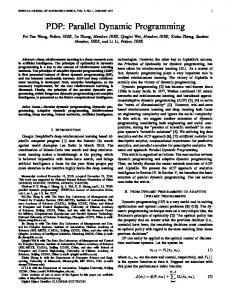
is s(v) = χ(v) ∩ χ(father(v)) (where father(v) is the father of v in T or ∅ for the root). The variables of χ(v) \ s(v) are said to be the proper variables of v. The rationale behind tree decompositions is that acyclic problems can be solved with a good theoretical complexity as it decomposes a master problem in subproblems (called clusters) organized as a tree. This is illustrated on the right, v ����� v ����� where the graph of a frequency assignment problem is covered by clusters (the sets χ(v)) defining a tree dev ����� composition. Locality of information v ����� v ����� in space or time often yield such nice v ����� decompositions in real problems. Different algorithms have been proposed to exploit such tree decomposiv v tions. We focus in this paper on elimination algorithms such as variable or ����� v v v bucket elimination (BE) [3, 1]. In BE, v a variable is chosen, all the cost funcv tions that involve this variable are v removed from the problem, and the marginal of the combination of these functions on the rest of the problem is added to the original problem. The problem obtained has one less variable and the same optimal cost as the original problem [3]. By repeatedly eliminating all variables, we ultimately get the optimal cost. One can show [5] that an implicit rooted tree decomposition lies behind BE and the complexity of the whole elimination process depends on this tree decomposition. Instead of eliminating one variable after the other, one may eliminate several variables at once. This is called block-by-block elimination [1]. Typically, all the proper variables of a leaf cluster v ∈ T are eliminated in one step. This is done repeatedly until the root cluster is eliminated, leaving the optimal cost to read as a constant. This approach has been sophisticated in Cluster Tree Elimination (CTE [5]) which may compute the marginals for each variable in two passes. Such algorithms have been parallelized in the context of inference, with no pruning [13]. 31
30
18
17
4
5
62
16
4
65
35
7
66
43
14
34
64
63
9
15
28
6
52
37
13
12
74
27
67
6
70
5
21
69
56
3
75
20
3
71
1
2
57
60
76
53
47
73
10
45
44
11
72
77
51
26
48
38
25
68
41
61
4
39
49
78
1
7
0
59
79
50
58
29
2
3
80
54
46
33
6
81
5
55
7
42
22
1
23
8
32
40
19
36
2
24
3
Parallelization of Block by Block elimination
In this paper, since we are just interested in computing the global optimum, we use the one pass block-by-block elimination algorithm described in [1] for optimization and adapt it to WCSP. Given an initial WCSP (X, W ) together with a tree decomposition (T, χ, ψ) of the WCSP, the elementary action of the algorithm is to process a leaf cluster v ∈ T , by eliminating all its proper variables: 1. we compute the marginal cost function F on the separator s(v): M F =( wS )↓s(v) wS ∈ψ(v)
2. we remove v from T , ψ(v) from W and all proper variables of v from X 3. we add F to both ψ(father(v)) and W As in BE, the problem obtained has less variables and the same optimum [1] and the updated triple (T, χ, ψ) is a tree decomposition of this problem. The process can be repeated on any leaf of the new tree T until an empty tree is obtained. The last marginal function F computed is a constant (a marginal on an empty set of variables) and its value is the optimum of the problem. Theorem 1. The time complexity for processing one cluster v ∈ T is O((|ψ(v)|+ #sons).d|χ(v)| ) and the space complexity is O(d|s(v)| ) where d is the domain size and #sons the number of sons of v in the original T . Proof. There are at most d|χ(v)| costs to compute and ((|ψ(v)| + #sons) cost functions in v. For space, there are d|s(v)| costs to store for the projection. The overall sequential complexity is obtained by summing on all clusters leading to a time complexity of O((e + |T |).dw ) and a space complexity of O(|T |.dr ) where w is the treewidth and r = maxv (|s(v)|) is the maximum separator size. To parallelize this algorithm, two sources of non determinism can be exploited. – The first lies in the computation of the marginal cost function F . It can be computed independently for each possible assignment t of the separator s(v) by assigning the separator variables with t in the WCSP (χ(v), ψ(v)) and solving the WCSP obtained using a state-of-the-art DFBB algorithm. – the second source of non determinism lies in the fact that the tree T may have several leaves. Whenever all the sons of a vertex v ∈ T have been processed, v becomes a leaf and can be processed. To get an idea of the speedups that can be reached in ideal (inexistent) conditions, we consider a PRAM machine with an unbounded number of cores, a constant time memory access, with a constant sequential setup time “s“ for starting a new process. Theorem 2. With an unbounded number of cores, the time complexity for processing one cluster v is O((|ψ(v)| + #sons).d|χ(v)−s(v)| ) + s.d|s(v)| ) and the space complexity is O(d|s(v)| ). Proof. The complexity of solving (χ(v), ψ(v)) after its separator assignment is O(|ψ(v)| + #sons).d|χ(v)−s(v)| ) since only |χ(v) − s(v)| variables remain unassigned. In parallel, the complete projection can be done in the same bound. The extra setup time for the d|s(v)| jobs is O(s.d|s(v)| ). Since a cluster v cannot be processed until all its sons have been processed, the overall complexity is controlled by the longest path from the root to any leaf where the length of a path is the sum of the processing times of its clusters. Compared to the sequential complexity, one see the impact of the sources of parallelism exploited. The separator assignment based parallization shifts complexity from an exponential in w (max. cluster size) to one in the maximum number of proper variables but we get an additive (instead of multiplicative) exponential term in r (max. separator size). The use of the T itself as a source of parallelism replaces a factor related to tree size by a factor related to its height.
4
Producing a suitable tree decomposition
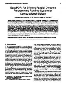
There has been a lot of work on tree decompositions. Usually, the problem considered is to produce a decomposition with a minimum treewidth, an NP-hard problem. We used Min-Fill and MCS heuristics, very usual heuristics aimed at the production of tree-decompositions with small treewidth [10]. Because of space complexity, separator size, instead of treewidth, is the main restricting factor for elimination algorithms. In our case, this is reinforced by the influence of setup times on time complexity. More precisely, for a separator s(v), the limiting factor is the associated separator space SS(v), defined as the size of the Cartesian product of the domains. These can be summed up over all v ∈ T to compute the overall separator space (and number of jobs) associated with the decomposition. We use decompositions with a bounded separator space. A traditional approach to get rid of a large separator is the so-called “superbucket” approach [5] which simply consists in merging the two separated clusters v and father(v) into one if the separator s(v) contains more than rmax variables. From the theoretical parallel complexity, one should a priori favor decompositions with a small maximum number of proper variables. However, time complexity is controlled by a tight (s.dr ) term for setup times and a much looser upper bound in O(dp ) for solving assigned problems. Therefore, the number of proper v ����� v ����� variables should not be too small or the overall time will be dominated by setup times. We therefore extend v ����� the “super-bucket” strategy, merging a cluster v with father(v) whenever v the number of proper variables of v is ����� smaller than a bound xmin . In the previously shown tree decomposition, we merge v3 and v4 bev v cause the separator space is too large, ����� v and similarly we merge v5 and v6 bev v cause v6 has too little proper variables, leading to the updated tree decompov sition in the figure on the right. Note that our elimination algorithm computes the cost of an optimal solution, but not the optimal solution itself. Producing an optimal solution afterwards can be done by solving each cluster once from root to leaves, using the projection of the optimal solution found for the father cluster on the separator of the current cluster as the initial values of the separator variables of the son. This takes less time than calculating the minimum cost itself. 31
30
18
17
3
5
62
16
4
65
35
7
66
43
14
34
64
63
9
15
28
6
52
37
13
12
67
74
27
70
5
21
69
56
75
20
3
71
1
2
57
60
76
53
47
73
10
45
44
11
72
77
51
26
48
38
25
68
41
61
39
49
78
1
0
59
3
79
50
2
7
58
29
80
54
46
33
5
81
1
55
7
42
22
23
8
32
40
19
2
36
24
5
Implementation and Results
To evaluate the practical interest of parallel block-by-block elimination, we have experimented it on hard decomposable problems. We preprocess a WCSP by
eliminating all variables with a small degree (2 or 3). An initial tree decomposition is produced by the Min-Fill and MCS heuristics [10]. For all values of rmax and xmin in [1, 25] and [1, 33] respectively, the super-bucket strategy is applied and the corresponding separator space SS and treewidth w are computed. If no decomposition with SS ≤ 2.106 exists, the method is said to be unsuitable for this instance. Else, we select a decomposition with minimum treewidth, unless an alternative decomposition exists that has a treewidth close to the minimum and a significantly smaller separator space (used for instances with a ∗ in the table below). The decomposition is rooted in the cluster with maximum |χ(v)|. This process has been applied to the CELAR radio link frequency assignment instances scen06, scen07, and scen08 (still open) and to hard genetics haplotyping instances, which have been tackled by a parallel AND/OR branch and bound approach in [9]. Name |X| d |W | w |T | SS rmax xmin The table on the right gives, scen06* 82 44 409 40 7 3.105 3 3 for each instance, the number scen07* 162 44 927 56 5 4.104 3 13 of variables, maximum domain scen08 365 44 1905 85 13 2.106 4 15 size, cost functions, treewidth, ped7* 293 4 667 141 28 2.105 14 5 number of clusters and separaped19* 484 5 1092 79 40 1.106 15 7 tor space obtained after preproped31* 513 5 1106 132 300 4.105 12 1 cessing and “super-bucketing” with corresponding rmax and xmin (using MCS for scen* and Min-Fill for ped*). The resolution of the WCSP (χ(v), ψ(v)) with a specific separator assignment is done using a Depth First Branch and Bound (DFBB) algorithm maintaining Existential Directional Arc Consistency [6] with a variable ordering combining Weighted Degree with Last Conflict [8] and using an upper bound produced by an initial restart strategy using Limited Discrepancy Search with a randomized variable ordering. Cost functions of arity above 3 are preprojected onto binary and ternary scopes. This corresponds to executing toulbar21 with options hlL. The parallel elimination process has been performed on a cluster with 400 cores (L5420 Xeon, 2.5 GHz with 4GB RAM per core) managed by the Sun Grid Engine. SGE uses a “fair share” strategy which may drastically change the number of cores allocated during execution. This makes a precise analysis of the effect of parallelization impossible. We therefore measured the CPU-time, number of nodes and backtracks of every toulbar2 execution. These times are used as input to a k-core simulator using real individual CPU- times. This simulation is played for different numbers of cores (k = 1, 15, 100, 1,000) using a 10 second job setup time for multi-core executions only (this is the scheduler interval used in the SGE configuration and it is consistent with real time: scen08 took less than 2 days to solve). Each job is in charge of solving 100 separator assignments. For two instances, solved with 100 reserved cores, we report the wall-clock time (inside parenthesis). We then give the CPU-time (on the same hardware, 1 core) of BTD-RDS [11], a state-of-the-art sequential branch and bound algorithm exploiting the same tree decomposition. A“-” indicates the problem could not be 1
http://mulcyber.toulouse.inra.fr/projects/toulbar2 version 0.9.1.2.
solved after 7 days. Finally, lower/upper bounds on the time needed to rebuild a solution on 1 core (sum of the min/max time in each cluster) is given. Name 1 core 15 cores 102 cores 103 cores Btd-Rds scen06 13h 08’ 1h 28’ 15’ 39” (20’ 53”) 3’ 32” 1’ 26” scen07 1d 6h 2h 09’ 23’ 27” (42’02”) 10’ 07” 1d 7h 3h 13’ scen08 127d 14h 8d 15h ped7 40’ 52” 22’ 55” 3’ 37” 35” 1’ 6” ped19 30d 3h 2d 2h 7h 32’ 58’ 18” 1d, 12h ped31 20’ 27” 41’ 03” 6’ 55” 1’ 25” 3h 37’
rebuild (l/u) 2’ 44”/2’ 47” 3’08”/3’ 10” 1h 32’/1h 37’ 11”/11” 1’ 17”/1’ 47” 44”/45”
For the smallest scen06 problem, which is easily solved using BTD-RDS, the approach is counter productive. For harder RLFAP problems, block elimination is capable of exploiting the full power of parallelism, enabling us to solve for the first time scen08 to optimality. The haplotyping problem instances ped7, 19 and 31 have been selected among the hard instances solved in [9] using a parallel AND/OR branch and bound with mini-buckets on similar CPUs. Our decomposition strategy gives again good results. If ped7 is too simple (less than 20 with BTD-RDS) to benefit from parallelization, for ped19 and ped31, we obtain good results. The elimination algorithm can be slower on 15 cores than on 1 core because of the 10” setup times. This is the case for ped31, because the 100 assignment jobs have a duration which is very short compared to setup time. In this case, a large part of the gain comes from the elimination algorithm itself, which is more efficient than BTD-RDS even in a sequential context. These times can be compared, with caution (these are simulated executions), with the best parallel (15 cores) times of [9]: 53’56”, 8h59’ and 2h09’ respectively: elimination, which is restricted to decomposable problems, gives better results on 100 cores. Contrarily to [9], which observed a large variability in the job durations, we observed a relatively limited variability of job durations inside a cluster. This could be explained by the small separator sizes (the different problems solved for a given cluster are not so different) and the upper-bounding procedure that adapts to each assignment. Note that sufficient separator space is needed to avoid starvation which occurs for example in scen07 on 1000 cores: scen07 defines only 400 jobs of 100 assignments. However, on the problems tested, job granularity seems relatively well handled by our super-bucket strategy. It could be improved by tuning the number of assignments per jobs according to the separator space, number of cores, tree decomposition topology and mean job duration.
6
Conclusion and Future Work
This paper presents a parallelization of an elimination algorithm for WCSP. The approach is suitable for difficult problems that can be decomposed into a treedecomposition with small separator size. This can be tested beforehand. Two sources of parallelization have been used in this process: the dominating one is based on partial problem assignments in separators, the second one comes from the branching of the tree-decomposition itself. The application of our prototype
on different real hard decomposable problems shows that a large number of cores can be effectively exploited to solve hard WCSP. This allowed us to solve to optimality the last CELAR radio link frequency assignment problem open instance. Obviously, more extensive experiments are needed on other decomposable problems. Beyond this, the most obvious way to improve the method is to tune the granularity of the jobs processed. We have used the super-bucket strategy and a fixed number of assignment solved per job to reach a suitable granularity, with good results on hard problems. Such tuning should ideally be done based on the problem at hand or even better, dynamically, as it is done in Branch and and Bound parallelization. Existing B&B parallization strategies could also be exploited inside each cluster resolution. Ultimately smarter scheduling strategies, taking into account precedences between clusters, could further improve the overall efficiency of the implementation. Acknowledgments: This work is partly supported by Toulouse Midi-Pyr´en´ees bioinformatic platform.
References 1. Bertel´e, U., Brioshi, F.: Nonserial Dynamic Programming. Academic Press (1972) 2. Cabon, B., de Givry, S., Lobjois, L., Schiex, T., Warners, J.: Radio link frequency assignment. Constraints 4, 79–89 (1999) 3. Dechter, R.: Bucket elimination: A unifying framework for reasoning. Artificial Intelligence 113(1–2), 41–85 (1999) 4. Dechter, R., Pearl, J.: Tree clustering for constraint networks. Artificial Intelligence 38, 353–366 (1989) 5. K. Kask, R. Dechter, J. Larrosa, A. Dechter: Unifying Cluster-Tree Decompositions for Reasoning in Graphical models. Artificial Intelligence 166(1-2), 165–193 (2005) 6. Larrosa, J., de Givry, S., Heras, F., Zytnicki, M.: Existential arc consistency: getting closer to full arc consistency in weighted CSPs. In: Proc. of the 19th IJCAI. pp. 84–89. Edinburgh, Scotland (Aug 2005) 7. Lauritzen, S., Spiegelhalter, D.: Local computations with probabilities on graphical structures and their application to expert systems. Journal of the Royal Statistical Society – Series B 50, 157–224 (1988) 8. Lecoutre, C., Sa¨ıs, L., Tabary, S., Vidal, V.: Reasoning from last conflict(s) in constraint programming. Artificial Intelligence 173, 1592,1614 (2009) 9. Otten, L., Dechter, R.: Towards parallel search for optimization in graphical models. In: Proc. of ISAIM’2010. Fort Lauderdale (FL), USA (2010) 10. Rose, D.: Tringulated graphs and the elimination process. Journal of Mathematical Analysis and its Applications 32 (1970) 11. Sanchez, M., Allouche, D., de Givry, S., Schiex, T.: Russian doll search with tree decomposition. In: Proc. IJCAI’09. pp. 603–608. San Diego (CA), USA (2009) 12. Schiex, T., Fargier, H., Verfaillie, G.: Valued constraint satisfaction problems: hard and easy problems. In: Proc. of the 14th IJCAI. pp. 631–637. Montr´eal, Canada (Aug 1995) 13. Xia, Y., Prasanna, V.: Parallel Exact Inference. In: C. Bischof, M. B¨ ucker, P.G. (ed.) Parallel Computing 2007. NIC, vol. 38, pp. 185–192. John von Neumann Institute for Computing (Sep 2007)