Communications for Statistical Applications and Methods 2016, Vol. 23, No. 2, 93–103
http://dx.doi.org/10.5351/CSAM.2016.23.2.093 Print ISSN 2287-7843 / Online ISSN 2383-4757
Tutorial: Dimension reduction in regression with a notion of sufficiency Jae Keun Yoo 1,a a
Department of Statistics, Ewha Womans University, Korea
Abstract In the paper, we discuss dimension reduction of predictors X ∈ R p in a regression of Y|X with a notion of sufficiency that is called sufficient dimension reduction. In sufficient dimension reduction, the original predictors X are replaced by its lower-dimensional linear projection without loss of information on selected aspects of the conditional distribution. Depending on the aspects, the central subspace, the central mean subspace and the central kth -moment subspace are defined and investigated as primary interests. Then the relationships among the three subspaces and the changes in the three subspaces for non-singular transformation of X are studied. We discuss the two conditions to guarantee the existence of the three subspaces that constrain the marginal distribution of X and the conditional distribution of Y|X. A general approach to estimate them is also introduced along with an explanation for conditions commonly assumed in most sufficient dimension reduction methodologies.
Keywords: central subspace, central kth -moment subspace, central mean subspace, dimension reduction subspace, regression, sufficient dimension reduction
1. Introduction High-dimensional data can arise in any place at any moment. It is common that useful information be extracted from such data for important decision making and that necessary statistical models be built to investigate the association between variables and prediction. In these cases, dimension reduction of data is inevitable to avoid obstacles like the curse of dimensionality. This is one reason why various dimension reduction techniques have been developed and remain popular. To have more intuition of necessity of dimension reduction, the prediction of Y is of main interest in the following regression of Y|X = (X1 , . . . , X p )T : Y|X = X1 + ε, iid
(1.1)
where (X1 , . . . , X p ) ∼ N(0, 1) ε ∼ N(0, 1) and stands for independence. By construction, the regression in (1.1) depends on X only through X1 regardless of the number of predictors, p. We consider the following two ways to predict Y. First, the response Y is predicted in the usual way of fitting the multiple linear regression Y|X ∈ R p and then doing prediction. The second way is to predict Y from a simple linear regression of Y|βˆ T X ∈ R1 , where βˆ ∈ R p is the ordinary least square coefficient vector estimated from the multiple linear regression. The clear difference between the two is placed on the dimension of predictors used in fitting the regression. The dimension in 1
Department of Statistics, Ewha Womans University, 52, Ewhayeodae-gil, Seodaemun-gu, Seoul 03760, Korea. E-mail:
[email protected]
Published 31 March 2016 / journal homepage: http://csam.or.kr c 2016 The Korean Statistical Society, and Korean International Statistical Society. All rights reserved. ⃝
Jae Keun Yoo
94
0
4
0
4
−6
0
4
6 2 0 −6
−4
−2
Confidence Interval
4
6 4 2 0 −4 −6
−4 −6 −6
p=40
−2
0
2
Confidence Interval
4
6
p=30
−2
Confidence Interval
4 2 0 −6
−4
−2
Confidence Interval
4 2 0 −2
−6
0
4
−6
0
4
p=50
p=60
p=70
p=80
p=90
4
−6
0
4
Estimates
−6
0
4
Estimates
4 2 0 −6
−4
−2
Confidence Interval
4 2 0 −6
−4
−2
Confidence Interval
4 2 0 −4 −6
−4 −6 0
Estimates
−2
Confidence Interval
4 2 0
Confidence Interval
4 2 0 −2 −4 −6 −6
6
Estimates
6
Estimates
6
Estimates
6
Estimates
6
Estimates
−2
Confidence Interval
−4 −6 −6
Confidence Interval
p=20
6
p=10
6
p=5
−6
0
4
Estimates
−6
0
4
Estimates
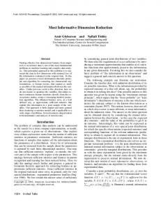
Figure 1: Prediction confidence interval in toy regression; black, usual multiple linear regression fit; red, dimen-
sion reduction linear regression fit.
the former is p, while it is always 1 in the latter where the dimension of X is reduced from p to 1. Prediction confidence intervals are computed to compare the performances between the two with varying p = 5, 10, 20, 30, 40, 50, 60, 70, 80, 90 (Figure 1). The sample sizes in all cases were n = 100. Figure 1 shows that the differences between the two prediction confidence intervals are even larger, as p increases. This simple example shows that the dimension reduction should be inevitable in highdimensional regression. We now focus on dimension reduction of predictors X in regression. Especially, we will seek for dimension reduction of X without loss of information on selected aspects of the conditional distribution of Y|X. This type of dimension reduction approach is called sufficient dimension reduction (SDR) because a notion of reduction without loss of information is directly related to sufficiency. A regression is to study the conditional distribution of Y|X. Let FY|X (·) denoted as the distribution function of Y|X. The goal of SDR is to find lower-dimensional function of X, namely g(X) such that FY|X (·) = FY|g(X) (·).
(1.2)
Statement (1.2) indicates that two regression of Y|X and Y|g(X) are the same. We can equivalently consider Y|g(X) in order to study Y|X. That is, the lower-dimensional predictor g(X) can replace X without loss of information on the conditional distribution of Y|X, if statement (1.2) holds for g(X). To stress this more clearly, statement (1.2) is equivalently rephrased to the following independence
Dimension reduction subspaces and required conditions
95
statement: Y
X|g(X).
(1.3)
Statement (1.3) directly indicates that g(X) has the same amount of information on Y|X as X does. There are many possibilities regarding forms of g(·). In SDR, we consider a lower-dimensional linear transformation BT X of X, where B ∈ R p×q with q < p. Then the goal of SDR is to pursue a lower-dimensional linear projection BT X of the original p-dimensional predictors X such that Y
X|BT X.
(1.4)
In the past two decades SDR methods for regression have been rapidly developed. Most of them can be considered nonparametric because they do not assume a specific form of Y|X; however, mild conditions are required. Unlike many local nonparametric approaches, they can√often avoid the curse of dimensionality because their estimates are global and converge at the usual n rate. The goal of the paper is to provide a notion of sufficient dimension reduction. For this, the paper is organized as follows. Section 2 introduces dimension reduction subspaces and target dimension reduction subspaces depending on selected aspects of regression. Some existing conditions for them are also described. Section 3 is devoted to providing general approach of inference on the target subspaces. Common conditions required in most sufficient dimension reduction methods are introduced in Section 4. In Section 5, we summarize the work.
2. Dimension reduction subspaces and centrality Before starting this section, we set up four models for illustration purpose. For each model, the iid following variable configuration are commonly used: X = (X1 , . . . , X5 )T ∼ N(0, 1) ε ∼ N(0, 1). ∑ Example 1: Y|X = 5i=1 Xi + ε; Example 2: Y|X = X1 (X1 + X2 ) + ε; Example 3: Y|X = X1 + exp(X2 )ε; ∑ ∑ Example 4: Y|X ∼ B(m, p), where p = exp( 3i=1 Xi )/{1 + exp( 3i=1 Xi )} and B(m, p) stands for a binomial distribution with total m trials and a success probability p.
2.1. Central subspace For Examples 1–4 above, it can be seen that the conditional distributions of Y|X depend on X only ∑ ∑ through 5i=1 Xi , (X1 , X2 ), (X1 , X2 ) and 3i=1 Xi , respectively. Therefore, the following relation can be easily established: Example 1: FY|X = FY| ∑5i=1 Xi = FY|BT1 X , where B1 = (1, 1, 1, 1, 1)T ; Example 2: FY|X = FY|X1 ,X2 = FY|BT2 X , where B2 = {(1, 0, 0, 0, 0), (0, 1, 0, 0, 0)}T ; Example 3: FY|X = FY|X1 ,X2 = FY|BT3 X , where B3 = {(1, 0, 0, 0, 0), (0, 1, 0, 0, 0)}T ; Example 4: FY|X = FY| ∑3i=1 Xi = FY|BT4 X , where B4 = (1, 1, 1, 0, 0)T .
Jae Keun Yoo
96
Therefore, with BiT X, i = 1, 2, 3, 4, the goal of SDR is achieved for the four regressions, respectively. For Example 2, consider the following matrices along with B2 : BTc1 X = (X1 , X1 + X2 ) with Bc1 = {(1, 0, 0, 0, 0)(1, 1, 0, 0, 0)}T ; BTc2 X = (X2 , X1 + X2 ) with Bc2 = {(0, 1, 0, 0, 0)(1, 1, 0, 0, 0)}T ; ) ) }T ( {( 1 1 BTc3 X = X1 , X1 − X2 with Bc3 = , 0, 0, 0, 0 (1, −1, 0, 0, 0) ; 2 2 BTc4 X = (−X1 , X1 + 2X2 ) with Bc4 = {(−1, 0, 0, 0, 0)(1, 2, 0, 0, 0)}T . Define the two coordinates of BT2 X and BTci X as (x1 , x2 ) and (xci ,1 , xci ,2 ), respectively. Then, pairs of (x1 , x2 ) have one-to-one mapping with those of (xci ,1 , xci ,2 ) for i = 1, . . . , 4. That is, any choices of Bi can be perfectly converted B2 , and hence we have that FY|X = FY|BT2 X = FY|BTc X for i = 1, . . . , 4. Then, i which one should be chosen among the five candidates? The answer for the question is that any of the five should be good. Now we will see this choice problem in another direction. Define that S(B) represents a subspace spanned by the columns of B ∈ R p×q . It is easily seen that S(B2 ) = S(Bci ) for i = 1, . . . , 4. B2 and Bci are different; however, their column subspaces are all the same. The choice problem is then no longer an issue if we consider a subspace spanned by the columns of B to satisfy (1.4). Any orthonormal basis of the subspace should also be fine because all of them span the same subspace. Based on this discussion, we define a dimension reduction subspace as: Definition 1. A subspace spanned by the columns of B such that Y reduction subspace (DRS) (Cook, 1998).
X|BT X is called dimension
A DRS always exists because B can be the identity matrix. Then, another choice problem arises because a regression has two or more DRSs. In Example 2, the columns of {(1, 0, 0, 0, 0), (0, 1, 0, 0, 0)}T forms a DRS, but the columns of {(1, 0, 0, 0, 0), (0, 1, 0, 0, 0), (0, 0, 1, 0, 0)}T also does a DRS. To choose the minimal subspace among all possible DRSs should be desirable because the minimal one still have full information of Y|X. How then do we find the minimal one among many DRSs? We will consider the intersection of all possible DRSs defined as follows. Definition 2. If the intersection of all possible DRSs is a dimension reduction subspace, the intersection is called central subspace (Cook, 1998), SY|X . If SY|X exists, it is minimal and unique. Therefore, the recovery of SY|X is naturally the mainstream in SDR. The central subspace does not always exist. We will closely investigate the conditions to guarantee the existence of SY|X in later section.
2.2. Central mean subspace The central subspace is to provide a complete information of the dependence of Y|X, but certain aspects of Y|X may be of primary interest, not Y|X itself. Indeed, a regression problem is often understood by a study of the mean function E(Y|X). If so, investigating E(Y|X) through SY|X should be overwork because the scope of SY|X is usually expected to be larger than necessary. The regressions like Examples 1, 2 and 4 depend on X only through their mean functions, and hence the consideration of E(Y|X) is adequate to capture all information on Y|X. We now move our main interest from Y|X to E(Y|X). Then, in SDR context, we need to replace the original p-dimensional predictor by a lower-dimensional linearly transformed one without loss of
Dimension reduction subspaces and required conditions
97
information on E(Y|X). If so, one should recover a subspace spanned by the columns of B such that ( ) E(Y|X) = E Y|BT X ⇔ Y E(Y|X)|BT X, (2.1) where B is a p × q matrix with q < p. Based on this discussion, a mean subspace is newly defined. Definition 3. A mean subspace (Cook and Li, 2002) is defined as a subspace spanned by the columns of B ∈ R p×q to satisfy Y E(Y|X)|BT X. When the mean function has all information on Y|X, that is, satisfying Y
X|E(Y|X),
the regression is often called location regression. The location regression forms a large class of regression including many generalized linear models. Their special case is an additive-error regression model (such as usual multiple linear regression or single-index model) in which we have Y − E(Y|X)
X.
In this location regression, a mean subspace should be the primary target over SY|X . Since there can be many mean subspaces in a regression problem, intersecting all possible mean subspaces is required to obtain the unique and minimal one. Definition 4. If the intersection of all possible mean subspaces is a mean subspace, the intersection is called central mean subspace (Cook and Li, 2002), SE(Y|X) . The conditions to guarantee the existence of SE(Y|X) are the same as SY|X ; therefore, they are never a cause of concern in practice.
2.3. Central kth -moment subspace Recall Example 3. In the example, the regression depends on X only through X1 and X2 . Since SE(Y|X) , spanned by (1, 0, 0, 0, 0)T provides information of X1 alone, SE(Y|X) is inadequate to summarize the regression. However, the consideration of the second conditional moment of var(Y|X) = exp(2X2 ) along with E(Y|X) can characterize the regression and provide the same information as SY|X . That is, in Example 2, while SE(Y|X) is clearly smaller than necessary, SY|X may be larger than necessary. Expanding the idea of the conditional moments of Y|X like SE(Y|X) , we newly construct a dimension reduction subspace of X. This construction is similar to SE(Y|X) ; however, the goal is to reduce the mean function as well as variance function and up to the kth moment function, leaving the rest of Y|X as the nuisance parameter. If so, SDR pursues BT X for B ∈ R p×q with q < p such that, for i = 1, . . . , k, ( ) M (i) (Y|X) = M (i) Y|BT X , where M (k) (Y|X) = E[{Y − E(Y|X)}k |X] and M (1) is replaced by E(Y|X). Again, the statement of M (i) (Y|X) = M (i) (Y|BT X), i = 1, . . . , k, can be re-written as the following conditional independence statement: { } (2.2) Y E(Y|X), . . . , M (k) (Y|X) BT X.
Jae Keun Yoo
98
Following the discussion, a kth -moment subspace and the central kth -moment subspace (Yin and Cook, 2002) are newly defined as: Definition 5. A kth -moment subspace is defined as a subspace spanned by the columns of B ∈ R p×q such that Y {E(Y|X), . . . , M (k) (Y|X)}|BT X. Definition 6. If the intersection of all possible kth -moment subspaces is a kth -moment subspace, the intersection is called central kth -moment subspace, S(k) . Y|X If S(k) exists, it is unique and minimal. Also, under the conditions to guarantee existence of SY|X , Y|X S(k) exits and is therefore not a cause of concern. Y|X (k)
2.4. Relation of SY|X , SE(Y|X) , SY|X and non-singular transformation of X (k) If SE(Y|X) , SY|X and SY|X exist for a regression of Y|X, we have SE(Y|X) ⊆ S(k) ⊆ SY|X . Also, the Y|X following four relationships naturally hold (Cook, 1998; Yin and Cook, 2002):
S(1) = SE(Y|X) ; Y|X SE(Y|X) ⊆ S(2) ⊆ · · · S(k) · · · ⊆ SY|X ; Y|X Y|X lim S(k) = SY|X ; Y|X
k→∞
SE(Y|X) = S(k) = SY|X under a location regression. Y|X We normally expect that SE(Y|X) ⊆ S(2) = SY|X because the regression models for Y|X often depend Y|X on X only through the first two conditional moments. Let SX denote one of SY|X , SE(Y|X) or S(k) for a regression of Y|X. Then we have the following Y|X result for a non-singular transformation of X. Results 1. Let A be a p × p non-singular matrix and define that Z = AT X. Consider SX and SZ from two regressions of Y|X and Y|Z, respectively. Then, we have SX = ASZ . Suppose that Z = Σ−1/2 {X−E(X)}, where Σ = cov(X) and Σ−1/2 Σ−1/2 = Σ−1 . Then Z is a standardized predictor with mean vector equal to zero and covariance matrix equal to the identity matrix. Result 1 directly implies that SX = Σ−1/2 SZ . In most SDR methodologies, SX should be the primary target, but SZ is often restored first and then back-transformed to SX for computational stability. It should be noted that the dimension of SX and SZ are equal, although bases of SX and SZ are different. In SDR, any of SE(Y|X) , S(k) , or SY|X should be the primary target subspace. Hereafter, its diY|X mension (often called structural dimension) and orthonormal basis will be denoted as d and η (ηz for Z-scale predictors). The dimension-reduced linearly transformed predictors ηT X are also known as sufficient predictors.
2.5. Conditions to guarantee the existence of SY|X The central subspace may not always exist. Consider X = (X1 , X2 )T with X12 + X22 = 1. That is, X1 and X2 are uniformly distributed on the unit circle. Y|X = X12 + ε, where ε ∼ N(0, 1) X. The regression of Y|X above depends on X only through X1 . Therefore, the column of η1 = (1, 0)T forms a DRS. By construction of X, X12 = 1−X22 . a regression of Y|X = 1−X22 +ε is equivalent to the original one of Y|X = X12 + ε; therefore the alternative regression depends on X only through X2 with η2 = (0, 1)T .
Dimension reduction subspaces and required conditions
99
The column of η2 then also forms a DRS. It is easily seen that S(η1 ) ∩ S(η2 ) = O. The central subspace does not exist; however, two DRSs do. The existence of SY|X can be guaranteed by constraining the marginal distribution of X and the conditional distribution of Y|X. Results 2. Let S(α) and S(ϕ) be DRSs for Y|X. If X has a density f (a) > 0 for a ∈ Ω x ⊂ R p and f (a) = 0 otherwise, and if Ω x is a convex set, then S(α) ∩ S(ϕ) is a DRS. Result 2 directly indicates that SY|X exists in regressions, if X has a density with a convex support. Results 3. Let S(α) and S(ϕ) be DRSs for a location regression of Y|X such that Y X|E(Y|X). If X has a density f on Ω x ⊂ R p , and if E(Y|X) can be expressed as a convergent power series in the coordinates of X = Xk , E(Y|X) =
∞ ∑ k1 ,...,k p
k
ak1 ,...,k p X1k1 · · · X pp ,
then S(α) ∩ S(ϕ) is a DRS. Under a location regression, we have that Y X|ηT X ⇔ Y X|E(Y|ηT X). Result 3 requires E(Y|X) to be well-behaved and requires X to have a density not necessarily positive everywhere. Result 3 can be easily extended to the case with higher-order conditional moments upto k such that } { Y X E(Y|X), M(2) (Y|X), . . . , M(k) (Y|X) . Therefore, according to Results 2–3, its existence is not a crucial practical issue along with those (k) of SE(Y|X) and SY|X since the conditions to guarantee the existence of SY|X is mild. Cook (1998, Chapter 6.4) is recommended for proof or more information on Results 2–3.
3. General approach of inference on SX Inference on SX has two components to estimate the true structural dimension d and an p × d orthonormal basis matrix η. Usually, most SDR methodologies under certain conditions (which will be discussed later) construct a kernel matrix M ∈ R p×p ≥ 0 such that S(M) = SX . Next, M is spectral-decomposed as: M=
p ∑
λi γi γiT ,
i=1
where λ1 ≥ λ2 ≥ · · · λ p ≥ 0 and γiT γi = 1 and γiT γ j = 0, i , j. Typically, the structural dimension d is determined first. Since S(M) = SX , the rank of M is the same as d of SX . The rank of M is also equal to the number of non-zero eigenvalues among λ1 , . . . , λ p . This directly indicates that the structural dimension is equal to the number of non-zero eigenvalues of M, and d is determined via testing a sequence of hypothesis (Li, 1991; Rao, 1965). Beginning with m = 0, test the hypothesis of H0 : d = m versus
H1 : d > m.
Jae Keun Yoo
100
If H0 : d = m is rejected, increment m by 1 and redo the test. The test is stopped for the first time H0 : d = m is not rejected, and set dˆ = m. These sequential tests require statistics Λm to test under H0 : d = m, which are the sum of the ordered eigenvalues multiplied by n: Λm = n
p ∑
λi ,
m = 0, 1, . . . , (p − 1).
m+1
The large sample distribution of Λm depends on SDR methodologies. ˆ ηˆ becomes a set of eigenvectors corresponding to the first dˆ largest Once d is determined to d, eigenvalues such that ( ) ηˆ = γ1 , . . . , γdˆ . ˆ is an estimate of SX . Then, S(η)
4. Common conditions in sufficient dimension reduction methodologies Here we review crucial conditions in SDR. Using the relation of SX = Σ−1/2 SZ , the conditions are discussed with the regression of Y|Z rather than that of Y|X. Let ηZ ∈ R p×d be an orthonormal basis matrix of SY|Z .
4.1. Linearity condition The linearity condition is very common in SDR literature, which is: ) ( E Z|ηTZ Z = ν is linear in ν. The main role of the linearity condition has been understood to force subspaces spanned by the columns of kernel matrices M ∈ R p×p produced by SDR methods to be a proper subspace of SY|Z such that S(M) ⊆ SY|Z . Therefore, most SDR methods require the condition in their methodological development. This condition is guaranteed to hold if the predictors X are elliptically distributed (Eaton, 1986). According to Hall and Li (1993), it is shown that (with large p) the linearity condition may hold to a reasonable approximation in many regressions. Li et al. (2004) discuss that nonlinearity among the predictors can degrade the performance of most estimation methods, in some applications that yield completely misleading results. Therefore, it is required to investigate if the condition is satisfied. One popular way is to inspect a scatterplot matrix of the predictors. The condition then seems to be satisfied if all cells of the plot look quite linear. However, there may be a chance that unobserved nonlinearity among the predictors exists despite appearing quite linear. Transforming or re-weighting of predictors is typically done if this linearity condition does not hold. However, a transformation of high-dimensional predictors may be inconvenient or infeasible. The re-weighting is computationally intensive (especially if p is high) and causes a deletion of observations in the data. Recently, Shao et al. (2006) provides a new view of the condition with respect to an adaptive estimation of η in the following single index model: ( ) Y|X = g ηT X + ε, where g(·) is unknown link functions and ε represents random error.
Dimension reduction subspaces and required conditions
101
A regression of Y|X depends on X only through at most one linear combination ηT X ∈ R1 of the predictors. Therefore, the single index model can be considered as a special case of SDR. An adaptive estimator is an efficient estimator for a model that is only partially specified. We do not know the form of g(·) in the single-index model above. Therefore the model is partially specified, and an asymptotically efficient estimator of η is an adaptive estimator. For an adaptive estimators, one can read a seminal paper by Bickel (1982). According to Shao et al. (2006), linearity condition guarantees existence of an adaptive estimate of η in the single-index model. Therefore, linearity condition let η estimated with the same efficiency as the link function is known. Thus, the linearity condition seems to substitute for knowing the exact conditional distribution of Y|ηT X, which has the same as that of Y|X.
4.2. Constant variance condition Some SDR methods require the following constant variance condition along with the linearity condition: ( ) cov Z|ηTZ Z = QηZ , where QηZ is an orthonormal projection operator onto the orthogonal complement of S(ηZ ). To understand a role of the constant variance condition, the inverse conditional variance function cov(Z|Y) under linearity condition for ηTZ Z can be investigated as: { { ( ( ) } ) } cov(Z|Y) = E cov Z|Y, ηTZ Z Y + cov E Z|Y, ηTZ Z Y { ( { ) } ) } ( = E cov Z|ηTZ Z Y + cov E Z|ηTZ Z Y } ] [ {( ( ) ))2 ( = E E Z − E Z|ηTZ Z ηTZ Z Y + cov PηZ Z|Y [ {( } ] )2 = E E Z − PηZ Z ηTZ Z Y + PηZ cov(Z|Y)PηZ { ( ) } = E cov QηZ Z|ηTZ Z Y + PηZ cov(Z|Y)PηZ { ) } ( = QηZ E cov Z|ηTZ Z Y QηZ + PηZ cov(Z|Y)PηZ . Assuming that the constant variance condition holds additionally, it is simplified: cov(Z|Y) = QηZ + PηZ cov(Z|Y)PηZ . Under both linearity and constant variance conditions we have the following equivalences for I p − cov(Z|Y). { } I p − cov(Z|Y) = I p − QηZ − PηZ cov(Z|Y)PηZ = PηZ − PηZ cov(Z|Y)PηZ = PηZ I p − cov(Z|Y) PηZ . This implies that I p − cov(Z|Y) can provide some information on SY|Z . Cook (2000) discusses the constant variance condition as: the condition holds, if Z is normally distributed, or it approximately holds, if Z is elliptically contoured. Experience also shows that it is less crucial than the linearity condition; therefore, the condition can be inspected through a scatterplot matrix of the predictors. The predictors are transformed for normality like the linearity condition if the condition is not satisfied.
102
Jae Keun Yoo
4.3. Coverage condition The goal of linearity and constant variance conditions is to induce the relationship of S(M) ⊆ SY|Z . This indicates that any of the two or both do not guarantee an exhaustive estimation of SY|Z . To have the exhaustive estimation, S(M) = SY|Z is assumed to hold, which is called coverage condition. Different from the previous two conditions, it is not possible to investigate that the coverage condition holds in practice. In most SDR methods, either of linearity or constant variance conditions or both are first assumed to hold for guaranteeing that M spans proper subsets of SY|Z . Then the coverage condition is assumed for the exhaustive estimation of SY|Z .
5. Discussion In the paper, we introduce a notion of sufficient dimension reduction in a regression of Y|X ∈ R p . The goal of SDR is to replace the original predictors X by its lower-dimensional linear projection without loss of information on selected aspects of the conditional distribution Y|X. Depending the aspects, the central subspace, the central mean subspace and the central kth -moment subspace are defined as primary interest. The conditions to guarantee the existence of the three subspaces are discussed since the three subspaces do not always exist. A general estimation approach to estimate them is also introduced, and the conditions commonly assumed in most SDR methodologies are explained. In a sequence of the second tutorial, SDR methodologies will be introduced to estimate the central subspace, the central mean subspace and the central kth -moment subspace. For the central subspace, methods using the conditional moments of the inverse regression of X|Y are used such as sliced inverse regression (Li, 1991) and sliced average variance estimation (Cook and Weisberg, 1991). To estimate the central mean subspace, the ordinary least square (Cook, 1998), principal Hessian direction (Li, 1992) and iterative Hessian transformation (Cook and Li, 2002) are popular among many. The central kth -moment subspace is restored by the covariance method proposed by Yin and Cook (2002). Most of the methodologies have the large-sample tests to determine the structural dimensions. However, a permutation test will be studied, and one of its advantages is no requirement large-sample distributions. Real data analysis for the methodologies will be presented to illustrate how to apply the methodologies in practice, and the results will be compared. A seeded dimension reduction approach (Cook et al., 2007) will also be introduced to provide a neat solution of SDR to large p and small n regression.
Acknowledgments This works was supported by Basic Science Research Program through the National Research Foundation of Korea (NRF) funded by the Korean Ministry of Education (NRF-2014R1A2A1A11049389 and 2009-0093827). The author is specially grateful to Professor Jeong-Soo Park, Editor-in-Chief, Communications for Statistical Applications and Methods, for the invitation of the paper.
References Bickel P (1982). On adaptive estimation, Annals of Statistics, 10, 647–671. Cook RD (1998). Regression Graphics: Ideas for Studying Regressions through Graphics, Wiley, New York. Cook RD (2000). Save: a method for dimension reduction and graphics in regression, Communications in Statistics-Theory and Methods, 29, 2109–2121.
Dimension reduction subspaces and required conditions
103
Cook RD and Li B (2002). Dimension reduction for conditional mean in regression, Annals of Statistics, 30, 455–474. Cook RD, Li B, and Chiaromonte F (2007). Dimension reduction in regression without matrix inversion, Biometrika, 94, 569–584. Cook RD and Weisberg S (1991). Comment: Sliced inverse regression for dimension reduction by KC Li, Journal of the American Statistical Association, 86, 328–332. Eaton ML (1986). A characterization of spherical distributions, Journal of Multivariate Analysis, 20, 272–276. Hall P and Li KC (1993). On almost linearity of low dimensional projections from high dimensional data, Annals of Statistics, 21, 867–889. Li KC (1991). Sliced inverse regression for dimension reduction, Journal of the American Statistical Association, 86, 316–327. Li KC (1992). On principal Hessian directions for data visualization and dimension reduction: another application of Stein’s lemma, Journal of the American Statistical Association, 87, 1025–1039. Li L, Cook RD, and Nachtsheim CJ (2004). Cluster-based estimation for sufficient dimension reduction, Computational Statistics & Data Analysis, 47, 175–193. Rao CR (1965). Linear Statistical Inference and Its Application, Wiley, New York. Shao Y, Cook RD, and Weisberg S (2006). The linearity condition and adaptive estimation in singleindex regressions, Retrieved March 1, 2016, from: http://arxiv.org/pdf/1001.4802v1.pdf Yin X and Cook RD (2002). Dimension reduction for the conditional kth moment in regression, Journal of the Royal Statistical Society Series B, 64, 159–175. Received January 22, 2016; Revised February 24, 2016; Accepted February 24, 2016