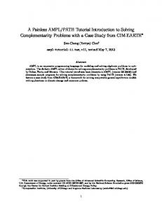
Tutorial Introduction to Layered Modeling of Software Performance Edition 3.0 Murray Woodside, Carleton University RADS Lab....http://sce.carleton.ca/rads
[email protected] May 2, 2002
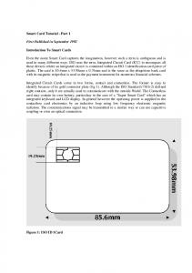
1.0 Software Server Concept We consider layered systems (software systems, and other kinds of systems too) that are made up of servers (and other resources which we will model as servers); the generic term we will use for these entities is “task”. A server is either a pure server, which executes operations on command (for instance a processor), or a more complex logical bundle of operations, which include the use of lower layer services. Such a bundle of operations may be implemented as a software server. requests for services e1, e2, etc reply message
common queue
A server entity (“task”):
Thread pool
• accepts requests from a single queue or mailbox • has one or more identical worker threads
e1
e2
choose different services e1, e2... “second phase” after sending reply
• executes one or more classes of service, labelled e1, e2, ... • ei makes requests to other servers • ei replies • optional “second phase of execution after the reply
FIGURE 1. The elements of a software server, including multiple threads, multiple entries, and second phases, which are all optional
1
Figure 1 illustrates the elements of a software server, as they might be implemented in a software process. The threads are servers to the queue, and the requests take the form of interprocess messages (remote procedure calls, or the semantic equivalent), and the entries describe or define the classes of service which can be given. The assumption in this theory is that each thread has the capability of executing any entryThe execution of the entry can follow any sequence of operations, and can include any number of nested requests or calls to other servers. Calls to internal services of the server are assumed to be included in the entry, so all calls are to other servers. A canonical sequence of operations is the first-phase/second phase sequence shown by the heavy line in the figure, with the reply sent after the first phase. Software servers often send the reply as early as possible, and complete some operations later a(e.g. database commits). The execution of the server entity is assumed to be carried out by a single processor, or multiprocessor, called its “host” and not shown in Figure 1. Once the request is accepted, the execution of the entry is a sequence of requests for service to the host and to other servers, and the essence of layered modeling is to capture this nesting of requests. Each request requires queueing at the other server, and then execution of a service there. The service time of a software server is the time to execute one reqeust, and it has two components, a phase 1 time until the reply is generated, and a phase 2 time. The “thread” abstraction in a software server can also model other mechanisms that allow the server to operate simultaneously on several requests, including a process pool, kernal or user threads, dunamically created threads or processes, and virtual threads. The abstract “task” model which applies to a software server can also be applied to other system resources, as described later. For instance, a disk device may offer more than one operation with different service times, modelled by entries; a buffer pool can be modelled by a set of “threads” each of which accepts one block of data and then tries to send it to the receiver entry. In the graphical notation adopted here for layered models, the server entity above is represented as in Figure 2. The multiplicity of threads is shown by a “stack” of task rectangles, which is optional. The requests are shown from entry to entry; the queue is not shown explicitly. The host may be shown as an oval; other devices such as disks are represented by a task to capture the services, and a host. The task part can represent multiple classes of services by the device, as entries.
2.0 Layered queuing concepts Modelers will be more familiar with non-layered models, so we will consider an example, and relate it to a layered model of the same system. A flat, non-layered model has only one layer of servers, and is equivalent to an ordinary queueing model. The following example has N User entities
2
client entry
entry e1
Task T
entry e2
host H FIGURE 2. Layered modeling notation for the server in Figure 1
making requests to a set of Server entities, and represents Users at workstations making requests to a central Server (file server or database server) with a printer and two disks. N User Entities [Z = 3 sec] 13
12
N User Workstations Shared Server CPU [s=5 msec.] [s = 15 msec.]
12
0.04 Network
7.1 0.6 Printer
Disk 2
Disk 2
FIGURE 3. Model with a single layer of resources (i.e., a plain queueing model) for a client-server system
The Users are the reference for performance measures, and execute a cycle in which they think for 3 sec in total (indicated by z = 3 sec.), and also make the indicated average number of requests to each server. These are the normalized parameters of a queueing network model (requests and thinking time per response), normalized to the reference popint of the Users. Each server has its own service time (indicated by s = value, for two of the servers) and discipline for serving requests. Layered approach In the layered view of the same model, shown in Figure 4, there are server tasks (which are not shown explicitly in a plain queueing model) on the server CPU, which have their own queues of messages to serve, and which in turn make requests to lower layer servers like the server CPU and disks. The Network also appears as a server which passes requests through, inserting its own latency and contention delays into the path. It connects messages to Server1 and Server2 through separate interfaces called entries, described below.The execution demand of Server1 and Server2 have the weighted average value of 15 msec shown in Figure 3 for the Server CPU.
3
N User Entities [Z = 3 sec] 13
7
5
N User Workstations
Network 1
1 Server1 Server2 [s=10 msec.] [s=22 msec.] 1
8.74
0.04
Shared Server CPU
0.6 Printer
7.1 Disk 2
Disk 2
FIGURE 4. Layered version of the client-server system
Readers who are familiar with queueing models will recognize this as an extended queueing model, with simultaneous resource possession. To execute operations at a server task the server task resource must be obtained, and then a device resource at the bottom. Layered queueing represents simultaneous resources in a simple canonical way. Resources, authority, layering Layered modeling describes a system by the sets of resources that are used by its operations. Every operation requires one or more resources, and the model defines a resource context and an architecture context for each operation. The architecture context is a software object to execute the operation, and the resource context is a set of software and hardware entities required by the operation. Every resource includes an aspect of an authority to proceed and use it, which is controlled by a discipline and a queue (which may be explicit or implicit). In layered modeling the resources are ordered into layers (typically with user processes near the top and hardware at the bottom) to provide a structured order of requesting them. With proper layering, a graph of all possible sequences of requests is acyclic, and deadlock among requests is impossible. For this and perhaps for other reasons, layered resources are very common in practice. Layering provides an ordering; notice that in this view requests may jump over layers. Tasks, entries, calls, demands The notation for layered queueing models uses the terms task, host processor, entry, call, and demand, as follows. • Tasks are the interacting entities in the model. Tasks carry out operations and also have the properties of resources, including a queue, a discipline, and a multiplicity. Tasks that do not receive any requests are special; they are called reference tasks and represent load generators or users of
4
the system, that cycle endlessly and create requests to other tasks. Separate classes of users are modelled by separate reference tasks. • A task has a host processor, which models the physical entity that carries out the operations. This separates the logic of an operation from its physical execution. Thus a disk is modeled by two entities, a disk task representing the logic of disk operations (including the difference between say a read and a write, and the logic of disk device-level caching), and a disk device. The processor has a queue and a discipline for executing its tasks, and a task has a priority. • A task has one or more entries, representing different operations it may perform. If the task is like a concurrent object, then the entries are like its methods (the name comes from the Ada language). Entries with different workload parameters are equivalent to separate classes in queueing. The workload parameters of an entry are its host execution demand, its pure delay (or think time), and its calls to other entries. • Calls are requests for service from one entry to an entry of another task. A call may be synchronous, asynchronous, or forwarding, as discussed below. This gives a rich vocabulary of parallel and concurrent operations, expressed in a manner very close to that of a software architecture description language. • Demands are the total average amounts of host processing and average number of calls for service operations required to complete an entry. More detailed descriptions, detailing the sequence of operations, can be given by giving the activity srtructure of an entry, described below. The most important graphical notation for layered queueing can be captured in the following diagram entry E1 Task T1 [Z = pure delay] [m = multiplicity] [s = hostDemand] [p = priority] ... by phases, [s1, s2] [d = discipline] Call (y = mean no of calls) ...by phases, (y1, y2) entry E2
T2
[s] [Z1] [Z2] P2
Processor P1 [m = multiplicity] [d = discipline] [relative speed]
FIGURE 5. Graphical notation for layered queueing... key elements
Figure 6 shows another example system, representing a web-based ticket reservation system. It uses the UML notation for the software in part (a) and the deployment in part (b). The layered model in part (c) combines these two.
5
Browser UserNode -interact( ) {delay = 5 sec} Browser WebServer
- connect( ) - display() - reserve() - confirm()
ServerNode WebServer TicketDB
TicketDB - queryTDB( ) - updateTDB( )
(b) UML deployment diagram
(a) UML class diagram
interact
Browser
[Z = 5 s]
connect display reserve confirm WebServer
UserCPU
queryTDB updateTDB TicketDB
ServerCPU (c) Layered Queueing model
FIGURE 6. Layered system example of a web-based ticket reservation system
6
3.0 Tools: the LQNS solver, the simulator, and their modeling language There are two solvers for layered queues, that take the same input format. One uses analytic mean-value queueing approximations to solve the queues at all the entities, while the other is a simulator. There is also an experiment controller that can execute parameterized experiments over parameter ranges. The analytic solver LQNS can be executed with the command line: lqns infile.lqn (where the suffix .lqn is suggested, but not mandatory) and it produces an output file with the default name infile.out. There are many options, which can be listed by invoking lqns or lqns -h. The documentation is the manual (“man”) page, also available in ASCII as lqns.txt. The simulator is invoked as: parasrvn [run controls] infile.lqn or: lqsim [run controls] infile.lqn and also generates an output file infile.out, which includes confidence intervals on the estimated performance parameters. Documentation is the man page for parasrvn, or the ASCII version parasrvn.txt. The experiment controller SPEX uses an expanded modeling syntax which includes parameter controls and selectors for performance measures. It is invoked as: spex infile.xlqn (where again the suffix .xlqn, standing for “extended lqn file”, is not mandatory) and it generates a set of case files, input and output, a summary called infile.res which tabulates the results over the cases, and optionally a set of plots of measures against parameter values. There is a documentation file called spex.txt. Model solver code for the reservation system in Figure 6 The file reserv-templ.lqn in the Appendix contains the reservation system example coded up for the lqns model solver. It has sections for general information (G), processor definitions (P), task definitions (T) and entry definitions (E). It is heavily commented to explain the meaning of each section, and the syntax of each statement. This is a template file for models based entirely on entries. Notice how every task must have a processor, and tasks are used to model many things: devices other than CPUs, external services that introduce a delay, users and their reaction time, critical sections and locks, buffers, etc. Jlqndef editor view The model is more easily edited and viewed with “jlqndef”. It provides windows with labelled fields for editing parameters and adding structure, and an automatic-layout view window for navigating the model and observing the structure. Jlqndef can be used with models that were created by manual editing or other means.
7
4.0 Task resources, queueing, and multiplicity (threads) An object may exist in a single instance, such that only one request can be served at a time; this is called a single-threaded task and is identified with a task resource, and a task queue. One task queue is used by all requests to all the task’s entries. This is an example of a “task” with both properties of an object providing operations, and of a resource. Some software objects are fully re-entrant, they can exist in any number of copies, each with its own context. These are often called multi-threaded, however because there is no limit to the number of threads we will term them infinite-threaded. This is an example of a “task” which imposes no resource constraint. An infinite resource is one which we do not have to consider as a resource at all, since it does not limit its authority to proceed. Some software objects exist as a pool of instances of a certain size. Requests are given a thread as long as there is one free; beyond this, requests must queue. These will be termed multi-threaded. Such a task models an object providing operations, and a homogeneous set of resource units that are dispatched from a single queue, like a multiserver. Multiple instances may be provided in different ways, for instance by process forking, by lightweight threads or kernel threads, by re-entrant procedure calls. A special case which is modeled as multiple instances is a single carefully written process that accepts all requests, and saves the context of uncompleted requests in data tables (this is virtual threading, or data threading). Multiplicity also applies to processors (single, multiple, infinite). All requests queryTDB updateTDB TicketDB queryTDB updateTDB TicketDB queryTDB updateTDB TicketDB
Queue for the Webserver task (not usually shown)
ServerCPU ServerCPU
connect display reserve confirm WebServer
A task has a single queue, for messages to all its entries
A multithreaded task running on a multiple processor
FIGURE 7. A Task queue, and multiple resources
8
4.1 Pseudo-tasks to represent modules (objects or subsystems) While an LQN task is used to model the resource aspects of a concurrent process as well as its workload, it can also be used to model just the workload aspects of an object or subsystem which is just part of a concurrent process, and which has no attached resource significance (we will call this a module). This can be helpful to structure the workload description around the software structure. If a task called T1 representing the overall container process makes a synchronous call (see below) to a task T2 representing a module which is part of the process, the model captures the fact that the process resources are held while executing the module. Sometimes a task representing a module will be called a pseudo-task, just to emphasize the fact that it does not have resources of its own. The pseudo-task is infinite threaded (see below), and is allocated to the same processor as the task that executes it.
5.0 Blocking calls and other styles of interaction Layered modeling in LQNS recognizes three kinds of interactions between entries: • asynchronous call: the sender does not wait and receives no reply. The receiving entry operates autonomously and handles the request. • synchronous call, with a reply. The sender waits (blocked) for the reply, and the receiving entry must provide replies. This is the pattern of a standard remote procedure call (RPC). The sending object task resource or thread is regarded as busy during the wait. Replies without blocking are modelled by introducing extra sender threads (these are model constructs), one for each potential outstanding reply. In the model these threads do block and wait for the reply, and they accumulate the total time to complete a response. These threads need not exist explicitly in the software (e.g. they may be virtual threads). • forwarding interaction: the first sender sees a synchronous interaction, and waits for a reply. However the receiver does not reply, but rather forwards the request to a third party, which either replies, or forwards it further. This gives an asynchronous chain of operations for a waiting client. Additional styles of interaction may be constructed using activities, including an asynchronous or delayed remote procedure call in which the sender continues at first, and eventually waits to get a reply. In each interaction there is a calling party, taking a “client” role and a called party, in a “server” role. A deeply layered system will have middle-level tasks that act both as servers, accepting calls from above, and as clients, making calls to lower-level servers. There may be tasks representing system users, that only originate requests. These pure client tasks act as sources of work, cycling between their own execution or delays, and requests into the system. The system may also receive an arrival flow of requests from outside; these are treated as asynchronous requests from the environment (there is no reply). To capture the response delay, we may introduce an artificial infinite threaded “response” task which serves the arrival stream, makes a synchronous request into the remainder of the system and waits for the completion of the activity.
9
Nested synchronous calls
interact
Browser
Forwarded query, replying directly to the client interact
[Z = 5 s]
external
Browser
display WebSrvr
[Z = 5 s]
synchronous
External arrivals, and an asynchronous invocation
synchronous sync
display WebSrvr
asynchronous
display WebSvr queryTDB TktDB
synchronous
forwarded
queryTDB TktDB
queryTDB TktDB
log
LogSrvr
[Z = 3 s] Layered Queueing notation for the three styles of interaction
Browser
WebSrvr
TktDB
Think Z=5 display
Browser WebSrvr
WebSrvr
TktDB
Think Z=5
TktDB
LogSrvr
display
display
queryTDB
queryTDB
queryTDB
log Think Z=3
UML Sequence Diagrams showing the messages passed. In this notation, the solid arrowhead shows a synchronous message, with a dashed arrow for the reply. FIGURE 8. Three styles of interaction in layered queueing models: LQNs and Sequence Diagrams
5.1 Workload parameters of an activity: summary so far An entry has one or more activities (so far we have only seen entries with a single activity), and the activities have workload parameters. The ones described so far are: • execution demand: the time demand on the CPU or other device (indicated by the token “s” in the modeling code)
10
• wait delay (also called a think time) (optional... it can be used to model any pure delay that does not occupy the processor) (token is Z) • mean synchronous requests to another entry (token is y) • mean asynchronous requests to another entry (token is z) Additional optional parameters, not discussed before, are: • the probability of forwarding the request to another entry, rather than replying to it, when serving a synchronous request (token is F) • the squared coefficient of variation of the execution demand requests. This is the ratio of the variance to the square of the mean; for a deterministic demand its value is 0 (token is c) • a binary parameter to identify a stochastic sequence in which the number of nested requests is random, with a geometric distribution and the stated mean, versus a deterministic sequence in which the number is exactly the stated number (which must be an integer). (token is f, with value 0 for stochastic (the default) or 1 for a deterministic sequence) To add detail to a model, we can introduce additional structure within an entry, called activities or phases. In the cases described so far each entry has just one activity or phase, with the parameters listed above. In the more general cases the same set of parameters can be used for each activity or each phase.
6.0 Performance measures: Service time and utilization values for an entry or a task. The service time of an entry is the time it is busy, in response to a single request. It includes its execution time and all the time it spends blocked, waiting for its processor and for nested lower services to complete. The service time in a layered model is a result rather than a parameter, except for pure servers. Since a task may have entries with different service times, the entries define different classes of service by the task. The overall mean service time of a task is the average of the entry service times (weighted by frequency of invocation). The utilization of a single-threaded task is the fraction of time the task is busy (executing or blocked), meaning not idle. A multi-threaded or infinite-threaded task may have several services under way at once and its utilization is the mean number of busy threads. A saturated task has all its threads busy almost all the time. Software Bottleneck A task which is fully utilized, when the resources it uses are not fully utilized, is called a “software bottleneck”. A typical example is a single-threaded task which blocks for I/O, and the typical cure is to multi-thread the task, making it a multiserver. Then when one thread is blocked another one can proceed. (See 1995 Software Bottleneck paper for more discussion).
11
interact
Browser
Browser
[Z = 5 s]
Think Z=5
(1)
WebSrvr
TktDB
display queryTDB
display WebSrvr Service time of the entry display of WebSrvr
(2) queryTDB TktDB
queryTDB
FIGURE 9. The service time of an entry includes any nested service times while it is blocked, waiting for a reply
7.0 Adding detail with activities within an entry Detailed description of the sequence of operations, when a task accepts a request at an entry, can be defined by describing activities with a precedence graph. The notation used in LQNS is: • Sequence:
activity1 -> activity2
activity 1 precedes activity 2
• AND-fork:
activity1 -> activity2 & activity3 & parallel (an AND-list of any length)
activity 1 precedes activities 2, 3... in
• AND-join:
activity1 & activity2 &.... -> activity3(predecessors are an AND-list of any length)
• OR-fork: one of
activity1 -> (prob2) activity2 + (prob3) activity3 +......means activity 1 precedes
• activity2 (with probability prob2) or • activity3 (with probability prob3) or ... (this is an OR-list of any length) • OR-join: length)
activity1 + activity2 -> activity3.....
• JOIN-FORK:
any OR or AND list -> any OR or AND list
• LOOP:
predecessor join-list -> (average-repeat-count)*activity1 activity2 ..... a repeated activity1, followed afterwards by activity2
12
(predecessors may be an OR-list of any
If the repeated part is a sequence, the rest of the sequence is defined as preceded by activity1. If it is a complex structure of activities it can be packaged into a separate pseudo-task (as described in Section 2.1), called by activity1. This pseudo-task can contain forks and joins and other behaviour structure nested within the loop. Task with activities Entry E2
Entry E1 a1
a9
AND-fork (p3)
a2
OR-fork (p4)
replies to E1 a5 [E1]
a3
OR-join
a4
a10 AND-join
a6
a7
a11 [E2] a8
*7.3 (3.2) a6 makes an average of 3.2 calls (synchronous messages) to SERV Service Entry SERV
LOOP: a8 is repeated an average of 7.3 times, then go to a11
replies to E2 after the join a12 a12 follows the reply
Task SERVT
FIGURE 10. A task with activities
If a request to an entry (say, entry1) generates a reply, then some activity in the graph triggers the reply. This is indicated by attaching the entry name to the activity, where it appears on the right of the arrow: • ...-> activity2[entry1] ...... activity2 is a reply-activity. When it is finished it sends a reply to the requester that initiated the execution of the entry. LQN code for the activity section The entries which use activities are identified in the entry list, along with the first activity in the entry. In a separate activity section for each task, the workload parameters of the activities and their precedence relationships are defined for all the entries that have activities. The template file activity-templ.lqn, repesenting a server with OR and AND forks, is commented to document to additional syntax for activities.
13
(Often there is a separate sub-graph for each entry. However, occasionally one may wish to define a single graph with multiple starting points at two or several entries, for instance to define a task which joins flows from two different tasks. For this reason each activity graph is defined for a given task rather than a given entry, and replies are indicated by entry name.) As well as the precedence graph definition, just discussed, the workload of each activity must be defined, using the parameters defined in Section 3.1. The template file template.lqn documents the syntax of the input file, including activities. Users {50} Task with activities Entry server serverStart OR-fork (0.4)
(0.6) parInit
seqInit
replies to call to server parReply[server]
parA AND-fork parB
LOOP
loopEnd
*3.5 loopOperation
replies to call to server seqReply[server]
LOOP *1.2
bigLoopDriver
loop2
LOOP: loopOperation and loop2 are repeated an average of 3.5 times, then go to loopEnd bigLoopStart
Task BigLoop, entry bigLoop
second first
fourth third
disk1read disk1write Disk1
disk2read disk2write Disk2
FIGURE 11. A server task with parallel and alternative activities, as defined in activity-templ.lqn
14
The activity diagram notation in UML is somewhat more general than the LQN notation, in that it allows a single graph to span multiple concurrent tasks, but it can be used to describe LQN activity graphs. However our purpose is focussed on defining performance models. Examples of activity notation are given in the document “Parallel Activity Notation in LQNS” by Franks (1999), which is also Chapter 6 in Franks thesis. The concurrency semantics of parallel activities assumes that a separate sub-thread (or its equivalent) exists for each parallel path. These sub-threads all compete for processing resources, and can block separately. Thus if one parallel path is blocked on a server, another one can run. Use activities for modeling detailed sequences: A basic use of activities is to described a particular deterministic sequence of execution steps of different lengths, and single requests to servers. Each step is modeled by its own activity. This provides a second level of detail, after making a model using average demands. Use activities for modeling parallel service: As shown in Figure 11, if a task makes two or more service requests (to other tasks) in parallel, so that it waits for both of them to complete before proceeding, this can modeled by using activities: • fork to parallel activities, one to make each request, • each parallel activity makes a blocking call for the service to one of the other tasks, and waits for the return, • join the parallel activities. This is discussed in the WOSP98 paper on modeling parallel service. Modeling Asynchronous RPC, and Prefetching: An asynchronous RPC is modeled by forking an activity to make the RPC, and joining at the point where the result is picked up by the main flow. Prefetches are modeled similarly, as are “futures” operations (which do a speculative computation in parallel).
8.0 Service with a Second Phase A wide variety of software services give a reply to the requester before they are entirely finished, in order to release the requester from the synchronous call delay as soon as possible. The remaining operations after the reply are done under sole control of the server task, and they form the second phase. A special shorthand is used to represent this common case. Entries with phase one and phase two can be represented by two activities, one performed before the reply and one after. Because they all have this simple structure they can be defined directly for the entry, without an explicit precedence graph. Each entry has a vector for each workload parameter, with a value for each phase. Thus the execution demand for the entry queryTDB above would be defined by a line beginning with code “s” for execution demand: “s queryTDB 0.3 0.5 -1”
15
WebSrvr
display WebSrvr
TktDB
display WebSrvr
display queryTDB
First phase, demand 0.3 s Second phase, demand 0.5 s
(1) queryTDB TktDB [0.3, 0.5]
(1) queryTDB phase1 [0.3]
TktDB
[queryTDB]
phase2 [0.5] Behaviour
LQN with phases in TktD LQN with activities in TktDB (activities shaded)
FIGURE 12. A second phase of service lets the client of the interaction proceed
The host demands are 0.3 for phase 1, 0.5 for phase 2. Note that the separator -1 is used in many places in the definition language. Second phases are common. An example is seen in a write operation to the Linux NFS file server; the write operation returns to the requester once the file is buffered in the server, and the actual write to disk is performed later, under sole congtrol of the server. Doing the writes in first phase would be safer, because the client would be told if the write failed, and this is how the NFS protocol was originally defined. Other NFS implementations allow second-phase or delayed writes only if the server has a battery-powered buffer to provide security of the data, in case of a power failure. Second phases improve performance; they give less delay to the client, and they increase capacity because there can be some parallel operation between the client and the server. The amount of gain depends on circumstances (real parallelism needs separate processors, and a saturated server cannot increase its capacity). The extreme case of all execution being in second phase is a kind of acknowledged handover of data from the client to the server. Thus it is similar to an asynchronous message, except that the sender waits for the acknowledgement. One important advantage of this is that the sender cannot over-run the receiver; the sender is throttled by the waiting for acknowledgements. Results for second phase at a single server, and at two layered servers : to come If some of a task’s work can be put into the second phase, the task can return more quickly to its clients. However if the task is already saturated the clients have to wait for many other services anyway and the advantage is small or even nil. The degree of improvement thus depends on the
16
degree of saturation,and where the saturation is. Table 1 shows how a group of users with a 5-sec thinking time are affected when the server service time is split between phase 1 and phase 2 in different ratios (LQNS approximate results). At low utilizations, more phase 2 is uniformly better, but as utlization increases, the best split moves towards the middle.
TABLE 1. The impact of dividing a unit server demand between phase 1 and phase 2 Response time (sec) for different values of demand s = [phase 1, phase 2] nusers
s = [0,1.0]
[0.2, 0.8]
[0.4, 0.6]
[0.6, 0.4]
[0.8, 0.2]
[ 1.0, 0]
1
0.166
0.310
0.464
0.629
0.807
0.999
4
1.125
0.726
0.827
0.996
1.269
1.6420
7
3.066
2.694
1.5087
1.7928
2.269
2.9256
10
4.8474
4.2741
3.8951
3.98149
4.4927
5.221
15
9.9096
9.4738
9.2281
9.2289
9.5048
10.037
20
14.9381
14.541
14.323
14.318
14.548
15.0120
Modeling finite buffers: A finite buffer space, which blocks its senders when it is full, can be modeled by a multi-threaded buffer task with second-phase interactions going into and coming out of the buffer. Each buffer space is modeled by a “thread” which immediately replies (releasing the sender) and then sends to the receiver (and waits until the receiver replies, to acknowledge receipt).
sender
Sender
Sender
Receiver
store
(2,0) store
Buffer
Buffer
receive
B threads
Receiver is busy
(0,1) receive Receiver [0, work] FIGURE 13. Modeling a finite buffer with blocking by a pool of B threads. The buffer is full at the time of the second store.
Modeling pipelines, using a third phase: In a software pipeline each task has three parts to its processing; input, processing and output to the next stage. Because LQN workloads are described by average values for each activity, it may be important to separate these three rather than lumping them together.
17
This is particularly clear in a pipeline with acknowledged handovers. Part 1 takes the message and acknowledges it to release the sending stage. Part 2 does the processing. Part 3 sends the output message and may have to wait for the acknowledgement. If the output message were averaged into the Part 2 workload, then on average it would occur in the middle, and this would give an error in the stage delay of a factor of nearly 2. In order to facilitate pipeline modeling with phases, a third phase has been made permissible, to model the output activity.
9.0 Logical resources (critical sections, locks, buffers) The task entity in layered modeling is used to model any resource whatever. Buffers have been discussed above. Consider a critical section shared by processes on the same processor, in which all the processes execute the same code in the critical section (this is like a monitor); it can be modeled exactly as a task. the critical section code and workload, including I/O operations and messaging, is associatetd with the critical section task rather than the caller process. If the processes execute different operations in the critical section, then the critical section “task” is an empty shell with no execution of its own, and with an entry for each caller... this entry calls a sort of shadow task defined for each process, which represents the critical section workload of that process. Only one of these shadow tasks can be active at once, and a queue of requests forms before the criticial section “task”. Effectively the calling processes are split into a component for the workload outside the critical section, and acomponent inside. If a caller is a multithreaded processes, or asynchronous (infinite-threaded) processes, the shadow task for it has the same number of threads. The same approach can be applied to locking a table. A full lock system, with many separate locks, and read and write locks, requires special treatment. The queuing disciplines are somewhat arcane, and there are too many locks to represent each one separately. This is a subject of current research. Memory and buffer resources can be modeled similarly, with a multiple “task” (the same designation as a multi-threaded task) to represent the resource, and with entries to activate the workload for each user.
10.0 Limitations This is not a complete list, but notes some limitations that have come up: • recursive calls are excluded (a task calling its own entries)... the approach for dealing with recursive calls is to aggregate the demand into the first entry. Possibly this should be accommodated, but it requires an assumption that the same thread handles the recursive request (to avoid deadlock when threads are limited), which limits the behaviour of an entry. • replication of subsystems (without defining all the replicas separately) is handled but only with restrictions; a thesis is available (Amy Pan).
18
• activity sequences which fork in one task and join in another can be solved by the simulation solver (parasrvn) but the analytic solver lqns has been inadequately tested for these cases, and may fail in various ways. • external arrival flows may be specified into an entry, however a system with only external arrivals causes problems for the analytic solver. It is reccommended to define sources of traffic as tasks which make requests and block; this has the advantage that it never overruns the system. To obtain a source with a given throughput define a very large source population (size N) with a long thinking time Z between requests, and it will generate an arrival rate of roughly N/Z per sec. If it deviates greatly, this indicates that the system is heavily loaded. • message loss is not modeled; current research may cure this. • exceptions and timeouts are also not modeled, similar comment.
11.0 Reference material See the web pages • www.sce.carleton.ca/rads... for material on the larger project (RADS is the Real-time And Distributed Systems group at Carleton), and for software download. • www.sce.carleton.ca/rads/lqn/documentation • www.sce.carleton.ca/faculty/woodside for my bibliography material Particularly recommended are: •the Quality conference paper in 97, for an overview, •the database modeling paper at ICDCS97, for a complete and rather complex case study, •the software bottleneck paper in 95 for a discussion of saturation effects, •the parallel service paper at WOSP98, regarding parallel services •Examples of activity notation are given in the document “Parallel Activity Notation in LQNS” by Franks (1999).
12.0 Running the tools LQNS has been compiled for Solaris, HP-UX and Linux, and for NT (actually, for GNU tools under DOS), It has a comprehensive manual page describing many options for diferent solver algorithms, for tracing solutions and for printing more or less detail. The best reference on the many solver options is Greg Franks’ PhD thesis (1999). The LQNS input language is essentially documented by the comments in the example files ... . There is a BNF definition included in the more extensive discussion of acivity notation, in “Parallel Activity Notation in LQNS” by Franks. Jlqndef is a graphical and text-window-based editor which shows a simple diagram of the model. It requires Java 1.1.3 or higher, with the “swing components”. 19
There is a useful tool called SPEX which is included in the distribution, for running experiments over sets of parameters. SPEX is a Perl script. You have to edit the textual version of the input model,and add specifications for control, for extraction of results, and for reporting results. Sets of runs can be done over any combination of parameter variations, and results are automatically tabulated or plotted in Matlab. SPEX is documented in the spex.txt.
13.0 Questions • Throughput refuses to increase when I introduce more resources. Search for a saturated resource; it may represent a modeling error. For instance, if one introduces more users, one must also introduce more processors for them to run on. A simple expedient is to make any resource which should not be a limt, infinite. This is also solver-friendly, a infinite resources are easy. • Convergence: what if my LQNS solution does not converge? The symptom is that the convergence value for the iterations is greater than the set value, typically 10^-6. Sometimes, especially in heavily loaded systems, the iterative solver will cycle and not converge. One cure which is sometimes effective is to reduce the value of the under-relaxation coefficient in the solver controls, from a typical value of 0.9 or 0.7 to a low value, of say 0.1. This is intended to force convergence by reducing the step size. If this does not succeed, then as long as the convergence value is less than 0.1, the solution found has some reasonable relationship to the correct value. (The size of the convergence value is the largest relative change from one iteration to the next, of any of the variables in the model; it does not directly indicate the size of errors, but if the solution is in fact cycling around the correct solution then all relative errors are probably smaller than this). A method which is ususally not effective is to increase the number of iteration steps. The basic recourse for greater accuracy is to simulate. • Replication: how can I model a system with many repetitions of a subsystem within it? Provided the replications are identical in every respect, and divide all their interactions with the rest of the system equally, the replication feature of LQNS can give efficient solutions. The full documentation of this feature is in the Master’s thesis of Amy Pan. Briefly, any task can have a replication factor r, which means that multiple copies are created. If its processor has the same r, then each cophy has a separate processor. If it communicates with other tasks with the same r, it communicaties with just one of them, and the interactions are assumed to form r subsystems. Messages between tasks with different r must have values of fan-in (f) and fanout (o) such that the product of source (r times fanout) = destination (r times fan-in). These factors f and o describe the replication of the message arcs. Unfortunately replication does not work for models with activities, only with phases. • Odd results for multiple servers: if I run for a series of values of m for server multiplicity, I may see rising throughput; then for m= infinity, the throughput drops a bit. How come? The waiting time calculation for a multiserver is an approximation, and errors of a few percent are to be expected. The infinite server queue is solved exactly (no waiting). If the anomaly is worrying, try a more exact multiserver algorithm by using “pragma -Pmultiserver=conway”, but it will take longer. • Non-blocking systems: in my model the servers are asynchronous. A server processes each message, whether a request or a reply, and then takes whatever message comes next. I never blocks to wait for a reply. How to model it? Such a server is modeled with infinite threads, allowing one active thread for each uncompleted request it is processing. This may be called virtual threads or data threads, since the request context, if any , is managed by user data. 20
• Solution Time: my LQNS solution takes a long time (a minute is long for a few tasks; 10 minutes is long for any model). Possible reasons are: (1) poor convergence (see below)... you may want to reduce the iterations or simulate; (2) a huge number of classes, generated by having a lot of separate source tasks (“reference tasks” and lots of entries on worker tasks.... you could get faster results if the sources were combined into fewer tasks, with random splits to generate the requests they make into the service layers.(3) do you have a multiserver (not a reference task) with a large m (say, m> 20?)... or layered multiservers one above the other, with moderate m... multiserver solutions are only moderately expensive by the default algorithm, but the others cost more. You might consider whether it could as easily be infinite (if, say, its usage is well below the limit so the limit is not a factor). In any of these cases, you might try to simulate; there have been models that solved faster by simulation. • Cycles: what do I do if my model has a synchronous messaging cycle? LQNS will refuse to solve a model, however it can be instructed to ignore the cycle checker with the pragma -Pcycles=allow. It then solves the model with an implicit assumption that if deadlocks are possible, they do not occur or are resolved. The simulator (parasrvn) will take a model with cycles at any time, however if a deadlock occurs as a result of a cycle, the simulation stops without any diagnostic. • Delay: how can I get the result for delay from an input at one point, to a response completion somewhere else in the model? The cleanest approach is to introduce some special model elements: first, at the start of the response, introduce a pseudo-task R to capture the delay as its service time. It has zero demands (s = 0), has infinite multiplicity (code i) runs on its own processor or an infinite processor, has deterministic phases (f = 1) and makes one synchronous call to the input point to start the response. Second, create a forwarding chain through the model along the path of the response, so that the reply is created at the completion point; the reply goes back to the pseudotask R, and ends its blocking state. • Simulation accuracy: how can I tell how accurate my simulation is? It is essential to get confidence intervals out of the simulation. If you don’t know about these, you will have to consult a statistics text. Parasrvn will calculate confidence intervals for you, for all its results, if you run with the -A (automatic) or -B (batched) run options. These have the form -A,a,p,b or -B,n,b where b is a batch length in model time units, which should be say 100 times longer than the longest service time in your model, and n is the number batches (suggest 30, which is the max allowed). For A, a is the accuracy target in 5 of mean values, p is the confidence leveel
14.0 Appendix: Model files Model File reserv-templ.lqn G #Comments between quotes, as many lines as necessary “Layered Queueing Network for a Web-based Reservation System” #Convergence criterion, iteration limit, print interval, underrelaxation #Under-relaxation coefficient stabilizes the algorithm if less than 1 0.0001 500 1
21
0.5 # End of General Information -1 # Processor Information (the zero is necessary; it may also give the number of processors) P 0 #SYNTAX: p ProcessorName SchedDiscipline [multiplicity, default = 1] # SchedDiscipline = f fifo|r random|p premptive| # h hol or non-pre-empt|s proc-sharing # multiplicity = m value (multiprocessor)|i (infinite) p UserP f i p ReservP f p DBP f p DBDiskP f p ReservDiskP f p CCReqP f i # End of Processor Information -1 # Task Information: (the zero is necessary; it may also give the number of tasks) T 0 #SYNTAX: t TaskName RefFlag EntryList -1 ProcessorName [multiplicity] # TaskName is any string, globally unique among tasks # RefFlag = r (reference or user task)|n (other) # multiplicity = m value (multithreaded)|i (infinite) t Users r users -1 UserP m 100 t Reserv n connect interact disconnect -1 ReservP m 5 t DB n dbupdate -1 DBP t Netware n netware -1 ReservP t DBDisk n dbDisk -1 DBDiskP t ReservDisk n reservDisk -1 ReservDiskP t CCReq n ccreq -1 CCReqP i # End of Task Information -1 #Entry Information: (the zero is necessary; it may also give the total number of entries) E 0 # SYNTAX-FORM-A: Token EntryName Value1 [Value2] [Value3] -1 # EntryName is a string, globally unique over all entries # Values are for phase 1, 2 and 3 (phase 1 is before the reply) # Tokens indicate the significance of the Value: # s HostServiceDemand for EntryName # c HostServiceCoefficientofVariation 22
# f PhaseTypeFlag # SYNTAX-FORM-B: Token FromEntry ToEntry Value1 [Value2] [Value3] 1 # Tokens indicate the Value Definitions: # y SynchronousCalls (no. of rendezvous) # F ProbForwarding (forward to ToEntry rather than replying) # z AsynchronousCalls (no. of send-no-reply messages) # o Fanout (for replicated servers)(ignore this) # i FanIn (for replicated servers)(ignore this) # This example only shows use of host demands and synchronous requests s users 0 56 0 -1 y users connect 0 1 0 -1 y users interact 0 6 0 -1 y users disconnect 0 1 0 -1 s connect 0.001 0 0 -1 y connect netware 1 0 0 -1 s interact 0.0014 0 0 -1 y interact netware 1 0 0 -1 y interact ccreq 0.1 0 0 -1 y interact dbupdate 1.15 0 0 -1 s disconnect 0.0001 0.0007 0 -1 y disconnect netware 1 0 0 -1 y disconnect dbupdate 1 0 0 -1 s netware 0.0012 0 0 -1 y netware reservDisk 1.5 0 0 -1 s dbupdate 0.0085 0 0 -1 y dbupdate dbDisk 2 0 0 -1 s ccreq 3 0 0 -1 s reservDisk 0.011 0 0 -1 s dbDisk 0.011 0 0 -1 #End of Entry Information -1 Model File activity-templ.lqn #This template documents the use of activities in depth #It assumes familiarity with other features documented in reservtemplate.lqn # or in template.lqn G “Activity template” 1e-06 50 5 0.9 -1 P 0 p p p p -1
UserP f i ServerP s#processor sharing at the server Disk1P f Disk2P f
23
T 0 t User r user -1 UserP z 50 m 50 t Server n server -1 ServerP m 4#4 threads with activities t BigLoop n bigLoop -1 ServerP i #pseudo-task for a complex loop pattern t Disk1 n disk1read disk1write -1 Disk1P t Disk2 n disk2read disk2write -1 Disk2P -1 E 0 s user 1.0 -1 f user 1 -1 y user server 1 -1#one request to the server per cycle A server serverStart#entry server is defined by #activities, with the first one being serverStart A bigLoop bigLoopStart s disk1read 0.04 -1#operation time of this entry s disk1write 0.04 -1 s disk2read 0.03 -1 s disk2write 0.03 -1 -1
#Optional sections for definition of activities # One section for each task that has activities, beginning A TaskName # list of activity parameters, using the syntax for entry parameters, but # with just one value and no terminator -1 # : (separator), then a section for precedence among activities # Syntax for precedence: # a1 -> a2 for sequence # a1 -> a2 & a3 ... AND-fork (any number) # a1 & a2 ... -> a3 AND join # a1 & a2 ... -> a3 & a4 ... AND join followed by AND fork # a1 -> (prob2)a2 + (prob3)a3 ... OR fork (any number, with probabilities) # a1 -> meanCount*a2,a3....for a repeated activity a2, followed by a3 # (notice that activities that follow a2 are inside the loop) # a6[entryName] indicates that after a6, a reply will be sent # to entryName A
Server s serverStart 0.0#every activity that is used must have a host demand s seqInit 0.3 s parInit 0.1 24
s parA 0.05 y parA disk1read 1.3#average of 1.3 read operations s parB 0.08 y parB disk2read 2.1 s parReply 0.01 s loopOperation 0.1 y loopOperation disk1read 0.7 s loop2 0 f bigLoopDriver 1#exactly one call operation (deterministic) y bigLoopDriver bigLoop 1#trigger the pseudo-task for the complex loop s seqReply 0.005 s loopEnd 0 : serverStart -> (0.4)seqInit + (0.6)parInit; parInit -> parA & parB; parA & parB -> parReply; parReply[server];#reply for the parallel branch seqInit -> 3.5* loopOperation, loopEnd; loopOperation -> loop2;#this activity is also in the loop loopEnd -> 1.2* bigLoopDriver, seqReply;#big loop is executed avge 1.2times seqReply[server]#reply for the sequential branch -1 A BigLoop#activities for the loop pseudo-task # (a loop pseudo-task is needed if there is a fork-join within a loop) s first 0.01#execute f second 1#deterministic sequence in this activity y second disk1write 1 #exactly one file write on this branch y third disk2write 1#average of one write on this branch s fourth 0.13#execute only : bigLoopStart -> first; first -> second & third; second & third -> fourth; fourth[bigLoop]#generate the reply from the pseudo task, ending the loop op -1
25