Understanding and prediction of stable atmospheric boundary layers ...

Understanding and Prediction of Stable Atmospheric Boundary Layers over Land

G.J. Steeneveld

1

Promotor: Prof. dr. A.A.M. Holtslag

Co-promotor: Dr. ir. B.J.H. van de Wiel

Samenstelling promotiecommissie: Dr. A.C.M. Beljaars Prof. dr. ir. B.J.J.M. van den Hurk Prof. dr. M.C. Krol Prof. dr. G. Svensson

Hoogleraar in de Meteorologie, Wageningen Universiteit

Wetenschappelijk onderzoeker, Leerstoelgroep Meteorologie en Luchtkwaliteit, Wageningen Universiteit

ECMWF, Reading, Engeland Universiteit Utrecht, KNMI Wageningen Universiteit, Stichting voor Ruimteonderzoek Nederland Stockholm Universiteit, Zweden

Dit onderzoek is uitgevoerd binnen de Buys-Ballot Onderzoeksschool.

2

Understanding and Prediction of Stable Atmospheric Boundary Layers over Land

G.J. Steeneveld

Proefschrift ter verkrijging van de graad van doctor op gezag van de rector magnificus van Wageningen Universiteit, Prof. dr. M.J. Kropff, in het openbaar te verdedigen op dinsdag 16 oktober 2007 des namiddags te vier uur in de Aula

3

ISBN 978-90-8504-716-2

4

Voorwoord Daar is-ie dan, het eerste MAQ proefschrift uit de “netkous”, de koosnaam voor ons nieuwe Atlasgebouw. Na vele uren van schrijven, knippen, plakken, opmaken en heropmaken is het dan eindelijk gereed. Allereerst wil ik mijn promotor en initiatiefnemer voor dit promotieonderzoek Bert Holtslag bedanken voor zijn stimulerende vragen, ideeën en discussies. Vooral als je weer eens terugkwam van een conferentie, stond mijn computer daarna snel te loeien om weer een nieuw idee uit te werken, of weer nieuwe berekeningen uit te voeren. Verder wil ik je bedanken voor het stroomlijnen van menig van mijn teksten en titels, wat de kwaliteit erg ten goede kwam. Toen dit promotieonderzoek begon, stond GABLS net in de kinderschoenen, maar door jouw initiatief is het uitgegroeid tot een volwassen project en een mooi platform waarin het vakgroepswerk kan worden (h)erkend. Graag wil ik Bas van de Wiel bedanken voor zijn begeleiding van het promotieonderzoek. Jouw theoretische blik op de zaak en wetenschappelijke manier van schrijven geven altijd weer nieuw initiatief en scherpte aan het artikel. Naast mijn directe begeleiders wil ik ook een aantal andere mensen bedanken met wie ik heb samengewerkt: Jordi Vila, Thorsten Mauritsen, Gunilla Svensson, Larry Mahrt, Sukanta Basu, Carmen Nappo, Cisco de Bruijn, Erik van Meijgaard, Thijs Heus, en de participanten in de GEWEX Atmospheric Boundary Layer Study (GABLS). En natuurlijk ben ik ook veel dank verschuldigd aan hen van wie ik metingen heb mogen ‘lenen’ (tsja ik ben zelf nu eenmaal niet zo handig/practisch): Oscar Hartogensis, Wouter Meijninger, de deelnemers in het CASES-99 experiment, Marku Kangas, Sylvain Joffre, Daan Vogelezang, Fred Bosveld, Bert Heusinkveld, Willy Hillen, Frits Antonysen, en Wim van den Berg. Verder verdienen Gerrie van den Brink en Kees van den Dries speciale waardering voor hun ondersteunende werk waardoor de vakgroep draait als een geoliede machine. Verder was de week niet compleet zonder Adrie’s humoristische weekafsluiter. Naast alle collega’s wil ik ook de studenten (Marcel de Vries, Sander Pijlman, Marcel Wokke, Miranda Braam, Christine Groot Zwaaftink, Peter Baas en Bram van Kesteren) bedanken voor de leerzame samenwerking gedurende afstudeervakken en Bachelorafsluitingen. Op deze plaats wil ik graag een aantal fondsen, instellingen en bedrijven bedanken voor de sponsoring door middel van reisbeurzen en andere subsidies. Hierdoor werd het bezoeken van cursussen, workshops en symposia aanzienlijk vergemakkelijkt. Het fonds Landbouw Export Bureau 1916/1918 heeft bijgedragen aan mijn bezoeken aan het ECMWF, het 17th Symposium on Boundary Layers and Turbulence (San Diego) en de GABLS workshop in Stockholm. 5

Kipp en Zonen B.V. sponsorde mijn bezoek aan 5th Annual meeting of the European Meteorological Society (EMS) in 2005. De EMS verleende een reisbeurs voor de EMS2004 and EMS2006 (respectievelijk in Nice en Ljubljana). Verder heeft het International Centre for Mechanical Sciences te Udine mijn bezoek aan een zomerschool aldaar gesponsord. NWO betaalde een deel van de reis- en verblijfkosten voor mijn bezoek aan het MISU in Stockholm. Allen hartelijk dank. Verder wil ik mijn vrienden en ex-huisgenoten Richard (alias “Woest”), John, Aart, Jan, Anja, Hanneke bedanken voor de wetenschappelijke en ook minder wetenschappelijke discussies. Daarnaast zeg ik sorry tegen iedereen die tijdens ons avondeten op 16B al mijn grenslaagverhalen heeft moeten aanhoren. Ik weet zeker dat jullie zonder al te veel voorbereiding een examen voor een inleidend meteorologievak gemakkelijk kunnen halen. Tenslotte wil ik mijn ouders bedanken voor hun steun, support en interesse in mijn werk. En natuurlijk wil ik Célia bedanken. Het is geweldig dat je naar Nederland gekomen bent, en we gaan een mooie tijd tegemoet.

6

Abstract

Abstract The main objective of this thesis is to contribute to further understanding of the stable boundary layer (SBL) over land, and its representation in atmospheric models. A SBL develops during night due to radiative surface cooling. Observations in the SBL, and their interpretation are difficult since many different physical processes can play a role. These processes are turbulent mixing, radiative transport, a coupling of the atmosphere with the vegetation and underlying soil, drainage flows, gravity waves, fog, and aspects of land use heterogeneity. Therefore, the understanding and the representation of the SBL in weather forecast and climate models is relatively poor, especially for calm nights. In this thesis, a detailed column model of the atmosphere-land surface system is used to represent the atmospheric boundary layer over land and ice. As such, Large Eddy Simulation results and CASES-99 field observations are used for comparison and model evaluation. It turns out that the degree of land-surface coupling plays a key role in forecasting the SBL. Also, the sensitivity of the radiation transfer model to vertical resolution is examined. It is found that the SBL can be satisfactorily modelled (except for the low-level jet (LLJ) and intermittency of the turbulence) if the geostrophic wind speed, advection, subsidence, and vegetation and soil properties are known, and if relatively high vertical resolution is used near the surface (both in the soil and in the atmosphere). Furthermore, the column model is used to study the nighttime 2 meter temperature increase due to additional CO2 as function of wind speed. Observations show that the temperature increase is similar for windy and calm nights, although this is somewhat counterintuitive. Model results confirm that the temperature increase is indeed similar for windy and calm nights. Next, an intercomparison study of limited area weather forecast models (COAMPS, MM5, HIRLAM) is performed for CASES-99. Large errors occur in the forecasted minimum temperature, SBL height and diurnal temperature range. Models that account for a realistic interaction with the land surface are advantageous. A sufficient large model domain is required to forecast the LLJ, and the forecasted surface cooling is very sensitive to the choice of the radiation scheme, especially for calm nights. Overall, it is possible to upgrade the model performance by using the lessons learnt with the column model. This thesis also explores the role of orographic drag on the SBL. It is shown that orography of 10 m amplitude can generate gravity wave drag as large as the turbulent drag. Accounting for this in a forecast model gave the required cyclones filling, and a better forecast of the SBL structure and LLJ. The thesis concludes with studies of the SBL height. Dimensional analysis is used to derive a new and robust formulation for the SBL height for a broad range of latitude and landuse conditions.

7

Contents 1. Introduction and research questions ................................................................................ 11 1.1 The role of the Atmospheric Boundary Layer in the land surface climate .................... 12 1.2 Stable boundary layer processes and their basic interactions ........................................ 13 1.3 Problems in stable boundary layer modeling ................................................................. 17 1.4 Research Tools ............................................................................................................... 19 1.5 GEWEX-Atmospheric Boundary-Layer Study (GABLS) ............................................. 20 1.6 Research questions and contents .................................................................................... 21 2. Modelling the Arctic stable boundary layer and its coupling to the surface ................ 23 2.1 Introduction .................................................................................................................... 25 2.2 Reference case: model description and results............................................................... 27 2.3 Coupling to the surface: a heat diffusion scheme (Alternative I) .................................. 30 2.4 Coupling to the surface: a bulk conductance layer (Alternative II) ............................... 33 2.5 Conclusions .................................................................................................................... 37 3. Modelling the evolution of the atmospheric boundary layer coupled to the land surface for three contrasting nights in CASES-99 .............................................................. 41 3.1 Introduction .................................................................................................................... 43 3.2 Background .................................................................................................................... 44 3.3 Observational data.......................................................................................................... 47 3.4 Model description........................................................................................................... 48 3.5 Results and Discussion................................................................................................... 54 3.6 Conclusions .................................................................................................................... 62 Appendix 3A: Estimating the flux-profile relationships for CASES-99.............................. 63 Appendix 3B: Model Sensitivity to Resolution in the Soil and Applicability in Operational Models.................................................................................................................................. 63 4. Evaluation of limited area models for the representation of the diurnal cycle and contrasting nights in CASES-99............................................................................................ 65 4.1 Introduction .................................................................................................................... 67 4.2 Observations and synoptic conditions............................................................................ 69 4.3 Model descriptions and configurations .......................................................................... 71 4.4 Surface Temperature and Fluxes.................................................................................... 74 4.5 Atmospheric Profiles...................................................................................................... 81 4.6 Sensitivity to radiation schemes..................................................................................... 87 4.7 Alternative land-surface scheme and turbulent mixing.................................................. 90 4.8 Conclusions and recommendations................................................................................ 94 Appendix 4A: Model Description ........................................................................................ 95 5. Exploring the possible role of small scale terrain drag on stable boundary layers over land .......................................................................................................................................... 97 5.1 Introduction .................................................................................................................... 99 5.2 Background .................................................................................................................. 100 5.3 Theory .......................................................................................................................... 103 5.4 Evaluation with field observations............................................................................... 105 5.5 Model impact of small-scale terrain drag..................................................................... 107 5.6 Discussion .................................................................................................................... 113 5.7 Conclusions .................................................................................................................. 115 Appendix 5A: Derivation of wave stress ........................................................................... 115

8

6. On land surface temperature trends in calm and windy nights .................................. 117 6.1 Introduction .................................................................................................................. 119 6.2 Background .................................................................................................................. 119 6.3 Model and experimental set-up .................................................................................... 121 6.4 Results and discussion.................................................................................................. 122 6.5 Conclusion.................................................................................................................... 125 7. Diagnostic equations for the stable boundary-layer height: evaluation and dimensional analysis............................................................................................................. 127 7.1 Introduction .................................................................................................................. 129 7.2 Background .................................................................................................................. 130 7.3 Observations................................................................................................................. 132 7.4 Evaluation and parameter estimation ........................................................................... 136 7.5 Alternative formulation using dimensional analysis.................................................... 141 7.6 Conclusions .................................................................................................................. 147 Appendix 7A: Dimensional analysis for the stable boundary-layer height formula.......... 150 8. Comments on deriving the equilibrium height of the stable boundary layer............. 151 8.1 Introduction .................................................................................................................. 152 8.2 Background .................................................................................................................. 152 8.3 Observations and Results ............................................................................................. 154 8.4 Conclusions .................................................................................................................. 157 9. Summary, reflections and recommendations ................................................................ 159 9.1 Summary ...................................................................................................................... 160 9.2 Recommendations for further research ........................................................................ 163 9.2.1 Intermittent turbulence and periodic oscillations in observations........................ 163 9.2.2 Intermittency and oscillations in column models.................................................. 168 9.2.3 Collapse of turbulence .......................................................................................... 169 9.2.4 Transition periods ................................................................................................. 170 9.2.5 Model intercomparison: How to proceed? ........................................................... 170 References ............................................................................................................................. 172 Samenvatting ........................................................................................................................ 189 Curriculum Vitae ................................................................................................................. 193 Publications........................................................................................................................... 194 Buys-Ballot Research School Education Statement Form ............................................... 196

9

10

1. Introduction and research questions

Chapter 1 Introduction and research questions

11

1. Introduction and research questions 1.1 The role of the Atmospheric Boundary Layer in the land surface climate This thesis deals with the subject of Understanding and Prediction of the Stable Atmospheric Boundary Layer over Land. In this general introduction first the main diurnal structure and development of the boundary layer and its role in the land-surface climate is sketched. Next, the most relevant processes in the boundary layer, our current understanding and the current status and problems of stable boundary-layer modeling are addressed. Finally the research questions are formulated. The Atmospheric Boundary Layer (ABL) is the turbulent atmospheric layer adjacent to the Earth’s surface that directly ‘feels’ the effect of the diurnal cycle at the surface. In principle, the ABL is a turbulent layer, characterized by irregular swirls of motions, so called eddies. Usually turbulence consists of many different eddy sizes superimposed on each other. These turbulent eddy motions are generated by two mechanisms: forced convection and buoyancy. Forced convection occurs when a flow travels over a rough area (with obstacles as grass, trees, cities), and is forced to pass these objects. Wind shear is the source for turbulence in this case. Buoyancy is the effect that warm air parcels have a smaller density than surrounding colder parcels, and therefore they start to drift upward. A characteristic property of turbulence is its effectiveness in transportation. Therefore, the ABL plays a vital role in the exchange of heat, momentum, moisture and natural (e.g. CO2 and other greenhouse gases) and anthropogenic (e.g. pollutant emission) contaminants from the Earth’s surface to the free atmosphere above the ABL. In the daytime ABL, the sun heats the surface and the turbulence is dominantly driven by buoyancy. The boundary layer rapidly grows in the morning, and large convective eddies provide vigorous vertical mixing over typically 1-2 km depth. In contrast, at night, buoyancy suppresses the turbulence intensity (sink), so only forced convection is a source of turbulence. Therefore, the nighttime ABL is much shallower, typically 100-200 m deep. However, during weak winds the suppression of turbulence by buoyancy is larger than the production by wind shear, so as a result the turbulence vanishes. Then, other transport processes than turbulence appear to govern the boundary-layer structure. These are radiation divergence (Ha and Mahrt, 2003), gravity waves (Nappo, 2002), drainage flows, the low-level jet (Garratt, 1985), fog (Teixeira and Miranda, 2001), and heat conduction from the soil (Holtslag and De Bruin, 1988). Stable boundary layers prevail at night, but also during daytime in winter in mid-latitudes as well as in polar regions (Yagüe and Redondo, 1995), and during daytime over irrigated regions with advection. In addition to daily weather forecasts, the stable boundary layer is especially relevant for agriculture (minimum temperatures, surface frost, dew, fog), road traffic (fog and frost), air traffic (fog, low-level jet), and wind energy engineering. Bony et al. (2006) found that the polar regions, that are dominantly stably stratified during a long part of the season, warm 1.4-4 times faster than the global average, but a clear reason for this is unknown. Further research to stable boundary layer processes is thus necessary.

12

1. Introduction and research questions 1.2 Stable boundary layer processes and their basic interactions The stably stratified atmospheric boundary layer is governed by many physical processes, although their role is not a priori clear for each process until now, and some of them has been only qualitatively understood. Questions such as “What determines the nocturnal cooling timescale at 2 m?” have still not been completely answered (Pattantyús-Ábrahám and Jánosi, 2004). After sunset during clear skies, the Earth surface starts to cool due to net emission of long wave radiation. As such, the virtual potential temperature increases with height, which we call stable stratification. We will now briefly point out the relevant processes and explain their role (if understood). -Turbulence A key characteristic of the atmospheric boundary layer is the turbulent nature of the flow. A turbulent flow consists of swirls (eddies) of different scales. Large eddies absorb energy from the mean flow. These large eddies break up to smaller eddies and finally these eddies are so small that they are dissipated by molecular viscosity. All eddy motions of different length scales, from millimetres to the scale of the boundary-layer height, transport momentum, heat, humidity and contaminants. The turbulence intensity is influenced by wind shear and stratification (the Brunt-Väisäla frequency). During daytime the solar insolation heats the surface, and creates thermal instability and thermals. In contrast, in the SBL turbulence is suppressed by the stable stratification during calm nights. Then the turbulence is only produced by the mean wind shear; it is destroyed by buoyancy effects and (at a larger rate) viscous dissipation. As a result its energetics can be in a delicate and precarious balance, and extremely sensitive to changes in the mean wind profile (which shear is its energy source) and the mean temperature profile (which lapse rate severely limits its vertical motions). Not surprisingly, the similarity statements we can make about the structure of the PBL are then of different nature from those in a convective case (Wyngaard, 1985). -Long-wave radiative transfer Every object in nature that is above the absolute temperature minimum of 0 K, emits radiation. This also holds for the air in the ABL. The amount of radiation that is absorbed or emitted by an air layer depends on the emissivity of the air layer and its temperature. The emissivity depends on the concentration of absorbing gases such as water vapour, carbon dioxide, ozone. Due to temperature and emissivity differences between air layers, the emitted absorbed long wave radiation differs between the different layers, resulting in a net radiative flux. Especially in the stable boundary layer, the temperature gradients near the surface can become extremely large, and consequently the emitted radiation differs strongly between the different layers. The potential temperature at a certain level in the atmosphere is amongst others governed by the divergence of turbulent flux and the divergence of the net long wave radiative flux (Rodgers, 1967; Anfossi et al., 1976).

13

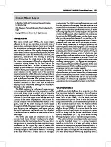
1. Introduction and research questions -Soil and vegetation On clear nights with weak winds, the boundary-layer energy budget is governed by radiative cooling and the compensating soil heat flux. The soil heat flux depends on the thermal conductivity and on the temperature gradient in the soil. Local soil properties, such as density, soil material, and soil moisture content, determine the conductivity. These properties can vary substantially in time and in space. However, in atmospheric models the soil is assumed to be homogeneous. In this thesis we will also assume a homogeneous soil. -Low-Level Jet Above the stable boundary layer, the wind speed profile is in the idealized case characterized by a small air layer with wind speeds larger than the geostrophic wind speed in the free atmosphere above the ABL. During daytime, the mean flow is determined by the pressure gradient force, the Coriolis force and the friction that is generated by the ABL turbulence. However, during sunset the turbulent drag suddenly decreases and the equilibrium is disturbed. As a consequence, the air accelerates in response to the lack of friction in the ABL. The low-level jet can act as a second source (beyond the production by near surface wind shear) of turbulence in the stable boundary layer due to the shear above and below the wind speed maximum. However, the nocturnal jet can also be formed or influenced by baroclinicity (i.e. the change of the geostrophic wind with height due to horizontal temperature gradients). -Gravity waves A general property of stably stratified geophysical flows is their ability to support and propagate gravity waves (Nappo, 2002). Einaudi et al. (1978) define gravity waves as essentially coherent structures (mainly horizontally propagating) with a speed mostly much less than of the mean wind with horizontal scales less than 500 km and times scales less than a few hours. Gravity waves can be generated by a variety of features: sudden surface roughness changes, convection, and undulating topography, on which we will focus here. Indeed these wave (type) motions are widely observed during special observational campaigns (e.g. CASES-99, Newsom and Banta, 2003). Since gravity waves are able to redistribute energy and momentum, they are important in determining the vertical structure of the atmosphere and the coupling of mesoscale motions to the micro scale phenomena. In essence, these waves transport positive momentum downwards. At a certain level, a socalled critical level can be reached (Fig. 1.1). Here the wind speed in the direction of the wave motion vanishes and consequently the wave breaks into turbulence. A similar mechanism can be present at the top of the stable boundary layer. In fact, this mechanism removes momentum from the mean flow, and thus acts as a drag on the flow (Chimonas and Nappo, 1989). Gravity waves can be generated by the topography of the land surface. These waves are standing waves, and the wave perturbations are not measured using standard eddy covariance technique, because the perturbations do not pass the sensor.

14

1. Introduction and research questions

Figure 1.1: Illustration of propagating gravity waves caused by orography. At a critical level (where the wind speed is 0), the waves starts to break up into turbulence. From Chimonas and Nappo (1989).

-Fog/ Moist processes When the surface cooling is strong enough, the air becomes saturated, and radiation fog starts to form over a certain layer. Next to the effect of the condensational heat release, the fog onset also rigorously modifies the radiative transport within the boundary layer and consequently the energy budgets of the boundary layer. The long-wave emission to space occurs at the top of the fog layer, which consequently cools rapidly. This destabilizes the fog layer, and the fog layer starts mixing. The final temperature profile follows the saturated-adiabatic lapse rate, with the surface now being warmer than the overlying atmosphere. Fog can prevail over large areas for a long time in polar regions. -Aspects of heterogeneity Land-surface heterogeneity (apart from orographic effects) can impact on the stable boundary layer. Natural landscapes are covered with patches of different vegetation and soil properties. Each of them will become in equilibrium with the local net radiative cooling. As such it might occur that differently stably stratified and unstably stratified patches exist next to each other. However, weather forecast models need to represent all patches within a single grid cell. Due to the non-linear nature of the turbulent exchange (e.g. Mahrt 1987; Ronda and De Bruin, 1999; Nakamura and Mahrt, 2006), grid cell averaging results in different and uncertain exchange coefficients compared to the local approach. Secondly, differential cooling due to land surface inhomogeneities might generate smallscale baroclinicity and consequently mesoscale circulations. These cannot be resolved in Numerical Weather Prediction (NWP) models, although these flows can generate wind shear and as such additional turbulent exchange.

15

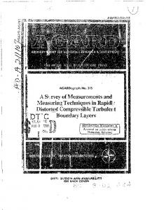
1. Introduction and research questions All small-scale processes as listed above need to be effectively represented in large-scale weather and climate models. It is clear that the parameterization of these processes is difficult. The present study focuses on a detailed modeling of the separate SBL regimes (according to the wind speed and surface cooling) and also aims to find the main physical cause of the transitions between the regimes (possibly in terms of external forcing parameters). To this end, we use a column-model with a detailed description of the transport by 1) turbulent exchange processes, 2) radiative processes and 3) soil-vegetation processes. This model has a parameterization of turbulence and the parameterization of radiative transport (emissivity approach). Furthermore a basic description is given for the atmosphere-vegetation/soil interaction by following the force-restore method (Deardorff, 1978) in combination with a canopy-resistance law. This description of the atmosphere-surface interaction will be improved by solving the diffusion equation for heat in the soil. An important aspect of the research is the comparison of the model results with observational data. For this purpose an excellent dataset is provided by the CASES-99 field experiment. The extensive cooperative field experiment CASES-99 (Cooperative Atmospheric Surface-Exchange Study) was carried out by various groups (Poulos et al., 2002), including the Meteorology and Air Quality Group of Wageningen University (e.g. Hartogensis and De Bruin, 2005). CASES-99 was especially designed to tackle the vexing scientific problems in stable and/or nocturnal atmospheric conditions (Nappo and Johansson, 1998). The experiment lasted for a full month, under various meteorological conditions, which makes the experiment extremely suitable to study the development of different SBL regimes. Fig. 1.2 illustrates the above mentioned processes, and their interactions. The main SBL forcings are the pressure gradient force, the Coriolis force, cloud cover, and free flow stability. For example, an increased geostrophic wind speed will enhance the turbulent mixing, and thus give reduced stratification (which can also occur due to incoming clouds). A reduced stratification will reduce the magnitude of the surface sensible heat flux in the weakly stable regime, and also limit the radiation divergence and thus the clear air radiative cooling. However, in the very stable regime, a reduction of the stratification might result in increased surface sensible heat flux. In both cases the surface energy budget is also altered, resulting in a modified soil heat flux. In the case of ceasing turbulence, the magnitude of the soil heat flux increases and vice versa. Moreover, this will alter the surface temperature and therefore the outgoing long wave radiation, and so the stratification. In addition, increased geostrophic wind will under certain conditions increase the impact of wave drag due to the orography, which at first increases the cyclone filling and thus reduces the geostrophic wind. On the other hand, it will also enhance the low-level jet wind speed (see chapter 5). This consequently might result in additional downward turbulent mixing from the jet. This starts to impact on the stratification again. The picture becomes even more complicated when radiation fog occurs. In principle, surface cooling can generate radiation fog when the air is sufficiently moist. However, with some wind, the latent heat flux will result in dew deposition, and heading off fog onset. Then in-

16

1. Introduction and research questions creased wind and turbulent mixing are necessary to transport moist air from above downwards for fog formation. Finally, when the fog becomes optically thick, the long wave cooling is at the top of the fog layer, instead of at the surface. Then the whole fog layer can become unstable with strong turbulent mixing. Overall it is clear that many complex interactions are present in the stable boundary layer. Free flow stability

Cloud cover

Pressure gradient

Coriolis force

LWD LLJ

Rad.div

Turbulent mixing

Wavedrag

2 Wind

1

Humidity LWU Ts

Stratification

1

Fog SENS HEAT FLUX

LAT. HEAT FLUX SOIL HEAT FLUX

2 Slope Orography

Roughness heterogene-

Soil temp. Figure 1.2: Overview of the relevant processes in the stable atmospheric boundary layer and their interactions. LWU and LWD are the upward and downward long-wave radiative fluxes, and LLJ the low-level jet. Positive interactions are full lines, negative feedbacks are dashed lines, and long dashed lines indicate a feedback that can either be positive or negative.

1.3 Problems in stable boundary layer modeling (partly adapted from Holtslag, 2006) For various applications in meteorology, agriculture and hydrology there is need for a better understanding and a better description of the ABL and of the energy and mass balance at the earth surface under stable conditions. It is commonly known that, currently, the poor parameterizations of the stable boundary layer (SBL) in weather and climate prediction models (Beljaars and Viterbo, 1994, 1998) are a direct consequence of the poor knowledge of the physical processes in the SBL (Mahrt 1999, 2001; Derbyshire, 1999). One reason for this is that a multiplicity of processes in the SBL and their coupling. At the same time it is realized that the current parameterisation of the SBL is still rather 17

1. Introduction and research questions poor, and that progress is slow (e.g. Beljaars and Holtslag, 1991; Holtslag and Boville, 1993; Beljaars and Viterbo, 1998). Unfortunately regional and global climate models show great sensitivity to the model formulation of mixing in stratified conditions. As an example, Viterbo et al. (1999) studied the vertical mixing in the ECMWF model in stable conditions. From two model runs with the same forcing conditions, but with (slightly) different stability functions in the mixing scheme, they noticed that differences in the mean winter temperatures at a height of 2 meters between the two model runs can be as large as 10 K over the continental areas! In addition, King et al. (2001, 2007) found similar results between model runs for winter climate over Antarctica. Also over Europe, it was found that significant differences occur between the 2-meter temperatures of a 30-year regional climate simulation with observations for present day winter climate (e.g. Lenderink et al., 2003). It also appears that the magnitude of the diurnal temperature cycle is typically underestimated over land. These results are to a large extent influenced by the boundary-layer scheme in stable conditions though other atmospheric processes (like clouds and radiation) and land-surface processes obviously also play a role (Viterbo et al., 1999). On the topic of stable boundary-layer diffusion it can be concluded that further research is needed to get more insight in how diffusion should be present at the grid scale of a large-scale model. Terrain heterogeneity, subgrid-scale orography and the coupling with the subsoil through the land surface scheme are major issues (Beljaars, 2001). This will be studied here. Climate models and weather forecast models need to make an overall representation of the smaller-scale boundary-layer and near surface processes. Besides the many different relevant processes in the stable boundary layer, the phenomenology of stable atmospheric boundary layers is also quite divers, e.g. shallow and deep boundary layers with continuous turbulence through most of their depth, and boundary layers with intermittent turbulence or even laminar flow. The small-scale processes influence the vertical and horizontal exchange of quantities between the surface and the atmosphere as well as the mixing in the atmosphere on a variety of scales. The overall representation of these processes and the related ‘spatial averaging’ is highly non-trivial due to the fact that there are many non-linear processes, and also because the environment has often a heterogeneous character on a variety of scales (Mahrt, 1987; Mahrt and Vickers, 2003). This normally is a motivation to allow for some ‘enhancedmixing’ in models as compared with tower observations (e.g. Beljaars and Holtslag, 1991; Holtslag, 2006). Fig. 1.3 shows the model performance for the 500 hPa. geopotential height of the ECMWF model with enhanced mixing (28R1_oper) and a turbulence parameterization based on field observations (MO_ejav). The model performance on the synoptic scale improves when the non-physical enhanced mixing is applied. On the other hand it is realized that the performance on the boundary-layer scale is less with enhanced mixing, since in that case the SBL is typically too warm, the LLJ is too weak and the SBL too deep. Another reason for having enhanced mixing is to prevent the models to enter an unphysical decoupled mode, which in turn may lead to run-away cooling close to the ground (Derbyshire, 1999; Steeneveld et al., 2006). In addition, it is known that turbulent mixing in stratified flow

18

1. Introduction and research questions has an inherent non-linear character and may, as such, trigger positive feedbacks. These positive feedbacks, in turn, may cause unexpected transitions between totally different SBL regimes (e.g. Derbyshire, 1999; Delage, 1997; Van de Wiel et al., 2002). Furthermore, we should realize the balance in building models: How much weight should be given should one give to the surface energy budget, to horizontal resolution, to turbulence closure, to PBL depth, or to the effect of stability on PBL structure? This is a difficult question. The complexity of all these components should match. We should perhaps be surprised if the first generation of experimenters had been able to perceive much order in the structure of the stable PBL (Wyngaard, 1985).

Figure 1.3: Anomaly correlation of the forecasted 500 hPa geopotential height in the ECMWF model for two different stable boundary-layer parameterizations (courtesy Anton Beljaars, ECMWF).

1.4 Research Tools The research tool we use in this thesis is a single column model (see Fig 1.4). Such a model represents only one column of the atmosphere, and is a prime tool for parameterization development and testing. This model type was chosen because it has some clear advantages compared to alternative model approaches. Its main advantages are that parameterizations can be tested without interference/feedback from the dynamics or other model components such as in 3D forecast models, and thus the physics can be tested in an isolated environment. In addition, the model is computationally fast compared to three-dimensional models (e.g. weather forecast models). Finally, a column model was preferred to Large-Eddy Simulation (LES) because the LES only resolves large eddies which are in minority in the SBL (especially for low wind speed), and thus with LES we would rely on the subgrid model. A recent paper by Beare and MacVean (2004) showed that for a moderately stable boundary layer, the turbulence statistics in LES starts to converge around 2 meter grid size, and thus requires large computational resources. Thus LES is only useful for strong winds. In addition, existing LES models 19

1. Introduction and research questions lack a coupling with the land surface and also radiative divergence is neglected.

Figure 1.4: Illustration of a single column representation of the atmosphere.

1.5 GEWEX-Atmospheric Boundary-Layer Study (GABLS) A part of the current work has been done in the context of GABLS, a project with the aim to improve the representation of the ABL in weather prediction and climate models. Within GABLS various single-column models from several research groups and operational weather centres, and ranging from first-order closure operational models to higher order closure research models, have done the same prediction task for a case with high wind speed. The results have been intercompared and also compared with LES simulations. These intercomparisons have the strong advantage that they improve the current knowledge in a way that could not be achieved by a single group.

b

a

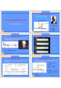
Figure 1.5: Model results (after 9 hours) for a stable boundary layer (a) potential temperature, b) wind speed as realized with several different parameterizations for the turbulent closure. The grey area indicates the ensemble mean results from LES (figures from Cuxart et al., 2006).

As an illustration of the GABLS results, Fig. 1.5 shows the model results for the first GABLS intercomparison study. This case is inspired by the LES study in Kosovic and Curry 20

1. Introduction and research questions (2000) for a SBL over ice, with a geostrophic wind of 8 ms-1 and prescribed surface cooling rate of 0.25 Kh-1. It is immediately clear that (even for a prescribed surface temperature) the models results diverge strongly. Also, most models produce a deeper SBL than the LES, and the LLJ is absent, or too weak, or at a higher altitude. In Chapter 2, we explore this case study with a more realistic boundary condition, i.e. for solving the surface energy budget. 1.6 Research questions and contents As sketched above, the prediction of the stable boundary layer in large-scale models has been a problematic feature for several decades. Despite the power of general circulation models in calculating the large-scale atmospheric flow, including advection and the effects of baroclinicity, they use too coarse resolution (both horizontally and vertically) to give a proper representation of the important small-scale processes in the stable boundary layer. Consequently, the parameterizations for the SBL in these large-scale models do not work satisfactorily. Before implementation of new parameterizations for large-scale models, these parameterizations should be tested in column mode against field observations. We want to know if the poor performance of large-scale models in stable conditions is a direct consequence of a poor understanding of real physical processes or that it is caused (merely) by problems of model resolution/computational restrictions. To investigate whether the stable boundary-layer physics can be modeled fruitfully on a local scale, we simulate three diurnal cycles of the CASES-99 measurement campaign with a single-column model, with very high resolution. Therefore, these simulations can be seen as a proof of principle of the current understanding of stable boundary-layer modeling. Only with a proper simulation of the stable boundary layer without constraints on the resolution, we gain confidence in our ability to understand the SBL. This will be discussed in Chapter 3. The confidence found in Chapter 3 was fair, and therefore we concluded that the physical processes at the local scale are well understood. Therefore an intercomparison and verification study with mesoscale models was conducted and reported in Chapter 4. Considering the physical processes, we shift to the following question: which physical process is lacking to forecast the stable boundary layer well in large-scale models? It is clear that the parameterized fluxes of momentum are highly uncertain, at one hand because of inaccurate boundary conditions (roughness length, subgrid orography parameter) and on the other hand due to uncertainties in the formulation for the stable boundary layer and subgrid orographic scheme. Quantitative verification on the level of momentum fluxes is virtually impossible (Beljaars, 2001). In Chapter 5, the role of orographically generated gravity wave drag is discussed as a possible missing mechanism in large-scale forecast models, and it will be shown that already smallscale orography can produce similar drag as the turbulence during calm nights. Finally, air quality prediction model results strongly rely on the calculated stable boundary-layer height. Pollutions released in the SBL cannot be transported over the inversion height that acts as a lid on the boundary layer and inhibits exchange with the free atmosphere.

21

1. Introduction and research questions The other way around, contaminants released above the boundary-layer height are confined to the free atmosphere and cannot be mixed into the boundary layer. Proper SBL height prediction is therefore a key issue in air quality predictions. This height is in practice calculated from meteorological variables at the surface and from atmospheric soundings. A well established SBL height formula is evaluated against four data sets with a broad range of latitude, surface roughness and land use. Consequently, by means of dimensional analysis an alternative model for the stable boundary-layer height is developed and validated with observations. Loosely speaking the thesis follows three paths. The first path considers the SBL from the one-dimensional perspective. The second path deals with the SBL in three-dimensional models, and the third part treats aspects and the modelling of the stable boundary-layer height. Thus the research questions and subquestions for this thesis are: Main question 1: To what extent do we understand the relative importance of the physical processes that govern the stable boundary layer, and can we model the stable boundary layer for different stability classes on the local scale? Subquestions •

To what extent is the stable boundary layer modelling sensitive to the coupling with the land surface?

•

To what extent is stable boundary layer modelling sensitive to resolution in the atmosphere and in the soil.

Main question 2: Is evaluation and intercomparison of three-dimensional limited area models useful and what do we learn? Subquestions •

How can we transfer forecasting skill on the local scale to the 3D large scale? Do we miss a physical process?

•

Which model descriptions are in favour for which atmospheric conditions?

Main question 3: How can we model the stable boundary-layer height? Subquestions •

How do diagnostic expressions for the stable boundary-layer height compare with observations, and can their performance be improved?

•

How should the relevant length scales in the stable boundary layer be combined to obtain an equation for the stable boundary-layer height?

22

2. Modelling the Arctic Stable Boundary Layer

Chapter 2 Modelling the Arctic stable boundary layer and its coupling to the surface1

This chapter has been published as G.J. Steeneveld, B.J.H. van de Wiel, and A.A.M. Holtslag, 2006: Modelling the Arctic stable boundary layer and its coupling to the surface. Bound.-Layer Meteor., 118, 357-378.

23

2. Modelling the Arctic Stable Boundary Layer Abstract The impact of coupling the atmosphere to the surface energy balance is examined for the stable boundary layer, as an extension of the first GABLS (GEWEX Atmospheric BoundaryLayer Study) one-dimensional model intercomparison. This coupling is of major importance for the stable boundary-layer structure and its development, because a coupling enables a realistic physical description of the interdependence of the surface temperature and the surface sensible heat flux. In the present case, the incorporation of a surface energy budget results in stronger cooling (surface decoupling), more stable and less deep boundary layers. The proper representation of this is a problematic feature in large-scale Numerical Weather Prediction and Climate models. To account for the upward heat flux from the ice surface beneath, we solve the diffusion equation for heat in the underlying ice as a first alternative. In that case, we find a clear impact of the vertical resolution in the underlying ice on the boundary-layer development: coarse vertical resolution in the ice results in stronger surface cooling than with fine resolution. Therefore, because of this impact on stable boundary layer development, the discretization in the underlying medium needs special attention in numerical modeling studies of the nighttime boundary layer. As a second alternative, a bulk conductance layer with stagnant air near the surface is added. The stable boundary-layer development appears to depend heavily on the bulk conductance of the stagnant air layer. This result re-emphasizes that the interaction with the surface needs special attention in stable boundary-layer studies. Furthermore, we perform sensitivity studies to atmospheric resolution, the length-scale formulation and the impact of radiation divergence on the stable boundary-layer structure for weak windy conditions. Keywords: Decoupling, GABLS, Radiation divergence, Resolution, Stable boundary layer, Surface energy balance.

24

2. Modelling the Arctic Stable Boundary Layer 2.1 Introduction In the first GABLS (GEWEX Atmospheric Boundary-Layer Study) model intercomparison study (Holtslag et al., 2003) a large variation for the outputs of single column models is found (Cuxart et al., 2006). As such, a simple stable boundary layer is studied with a prescribed constant cooling rate of −0.25 K h-1 at the surface. Such a forcing method for the stable boundary layer (SBL) is quite common (see e.g. Delage, 1974, 1997; Nieuwstadt and Driedonks, 1979; Kosovic and Curry, 2000). Alternatively, the surface turbulent heat flux w'θ' s can be prescribed (Galmarini et al., 1998, Viterbo et al., 1999). Although both methods are classical in the sense that they are easy to apply (especially in theoretical studies), there seems no direct physical justification for either one. In fact, the presence of feedbacks between the surface temperature (Ts), the surface sensible heat flux and the heat flux from the underlying medium towards the surface is essential (Derbyshire, 1999). Changes in surfacelayer stability will affect the sensible heat flux through the stability functions, and consequently, the surface temperature will be affected through a coupled surface energy budget. In the case of a surface energy budget, we can raise the question how the turbulent sensible heat flux in the SBL will react on surface cooling (Derbyshire, 1999; Delage et al., 2002). In fact the sensible heat flux may react in two different ways, corresponding to two regimes (compare also De Bruin, 1994 and Derbyshire, 1999):

•

The weakly stable case, in which the sensible heat flux increases with stability. A sudden increase in stratification leads to a larger heat flux, opposing the increased stratification (negative feedback).

•

The very stable case, in which an increase in stratification leads to a reduction of the sensible heat flux and therefore intensifying the increased stratification (positive feedback). This may lead to a collapse of turbulence so that the actual SBL decouples from the surface (ReVelle, 1993; Coulter and Doran, 2002; Delage et al., 2002; Van de Wiel et al., 2004). Note that besides of this subdivision, alternative SBL classifications have been proposed by Beyrich (1997), Mahrt et al. (1998), Van de Wiel et al. (2003) and Mahrt and Vickers (2002) and others. At present no general classification picture of the SBL exists. Therefore, in the current work we use the pragmatic subdivision indicated above, i.e: weakly stable and very stable conditions. From observations it is known that the SBL may either remain in a decoupled state, or recouple after a certain time, leading to turbulence of intermittent character (Van de Wiel et al., 2002a). From a modelling perspective, this very stable regime often leads to practical problems: for example large-scale atmospheric models tend to decouple and remain decoupled in an unphysical sense (e.g. Louis, 1979; Derbyshire, 1999). This can result in a serious cold model bias, especially during conditions where strong stratification exists for longer periods such as in the polar region in winter time (Viterbo et al., 1999). To circumvent this problem,

25

2. Modelling the Arctic Stable Boundary Layer large-scale atmospheric models apply artificial enhanced mixing formulations for turbulence in the case of strong stability (e.g. Louis, 1979; Beljaars and Holtslag, 1991). The importance of the surface-energy balance feedback was indicated by theoretical considerations above. The relevance of this feedback can also directly be inferred from typical observations of the surface temperature. Van de Wiel et al. (2003) illustrate from observations during the CASES-99 experiment that the surface temperature Ts, the turbulent heat flux and the soil heat flux may show simultaneous rapid changes during the night, revealing their interdependence. These fluctuations (with a rather high frequency compared to the daily cycle) are important for the dynamics of the SBL as a whole and cannot be modelled without taking into account the mutual interactions between the surface temperature, the sensible heat flux and the underlying soil. Derbyshire (1999) concludes: “Even the simplest valid analysis needs to couple the wind profile, the temperature profile and the surface heat budget”. Steeneveld et al. (2004) reveal that one-dimensional modelling results are largely improved as compared by detailed in situ observations when: a) an accurate vegetation layer and fine soil discretization are applied, and b) radiation divergence is included, at least for low geostrophic winds. Fig. 2.1 shows results of the modelled vegetation temperature (full line) for three consecutive diurnal cycles during the CASES-99 experiment (Steeneveld et al., 2004). The first night is intermittent turbulent (moderate stable), the second continuously turbulent (weakly stable) and the third night is ‘non-turbulent’ (very stable), with suppressed turbulence. Thus we cover a wide range of stability conditions in this experiment. A clear agreement is found between the model results and the observations for these three different types of nights. This result is remarkable given the fact that the surface temperature is a difficult quantity to predict accurately with an off line model, especially for such a broad range of stability classes (Best, 1998). Additionally, we find that (not shown) the modelled potential temperature (θ) profiles also compare well with boundary-layer observations for these particular case studies. The dash-dotted line in Fig. 2.1 shows the modelled surface temperature when the enhanced mixing approach is applied in the single column model, as is common practice in operational NWP and climate prediction models (e.g. Beljaars and Viterbo, 1998). Then the surface temperature is overestimated with about 5 K for the first two nights and the first half of the third night. Thus even from a practical point of view (as in NWP), the enhanced mixing approach is not appropriate over a large stability range. Fig. 2.1 shows that an accurate prediction of in situ observations is possible, using a sound physical representation of the soilvegetation, heat exchange processes, without the need for an (artificial) enhanced mixing formulation. Note that in our current comparison with local observations, we disregard possible enhanced mixing as a consequence of spatial averages issues such as addressed by Mahrt (1987) that may play an important role in NWP of SBL under heterogeneous conditions. The foregoing motivates us to pose the research question: what is the impact on the GABLS case study when we include realistic features of a surface energy balance? Therefore, we compare the outcome of the reference case (i.e. with prescribed surface cooling) with the

26

2. Modelling the Arctic Stable Boundary Layer results of two alternative surface coupled cases. Both alternatives explicitly solve the surface energy budget equation and apply •

the diffusion equation for heat in the underlying ice (Alternative I), or

• use a bulk-conductance law at the surface (Alternative II), in our extension of the single column model by Duynkerke (1991, 1999) to account for the heat flux from the underlying medium. This model also participated in the GABLS reference case comparison of various single column models (Cuxart et al., 2006). Section 2.2 gives a short overview of the model description and additional results for the reference case study. Section 2.3 presents the results for a coupled system with a heat diffusion scheme (Alternative I). Results for Alternative II are presented in Section 2.4. Conclusions and recommendations are given in Section 2.5.

Figure 2.1: Modelled (full line) and observed (+) vegetation temperature for the period 23-26 October 1999 (Day of Year (DOY) = 296.5-299.5) for the CASES-99 experiment. The dash-dotted line indicates the model performance when enhanced mixing is applied.

2.2 Reference case: model description and results a) Model description Our model is an extension of the model by Duynkerke (1991, 1999). Turbulent mixing is parameterised in terms of local gradients (assuming local equilibrium of the TKE budget): ∂X w' χ' = − K x , (2.1) ∂z

where X is a mean quantity and w'χ' the turbulent flux of X and z the height above the sur-

face. The eddy diffusivity (K) is given by first order closure, expressed as (see also Holtslag, 1998):

27

2. Modelling the Arctic Stable Boundary Layer l 2 ∂V Kx = φ m φ x ∂z

x ∈ {m, h}

(2.2)

with the mixing length l = k z and x = m for momentum and x = h for heat, k the Von Kármán constant and ∂V ∂z the vector wind shear. Based on reanalysis of the Cabauw tower observations from Nieuwstadt (1984), Duynkerke (1991) proposed the stability function  β φ x (ζ ) = 1 + β x ζ1 + x  αx

 ζ  

α x −1

,

(2.3) 3

where ζ = z Λ , Λ the local Obukhov length, defined as Λ = −θu*L /(kg w' θ') , and u*L the local friction velocity. Coefficients were found to be βm = 5, αm = 0.8, βh = 7.5 and αh = 0.8, as compared to the original findings by Nieuwstadt (1984) who found αh = αm = 1, and βm = βh = 5. Note that the coefficients used in the present study (viz. as in Duynkerke, 1991) are in close agreement with the prescribed coefficients for the surface layer in the intercomparison case, especially for the weakly stable part. Thus a simple first order closure model for turbulence is used in the present model, because the main aim of this paper is to illustrate the impact of coupling the atmosphere to the surface. Moreover, as shown by Brost and Wyngaard (1978), TKE transport terms in the SBL are usually relatively small so that the local equilibrium assumption is often applicable. Radiation divergence is neglected in the reference case. The GABLS reference case study is defined over an ice surface with a relatively large roughness length for momentum and heat of z0 = z0h = 0.1 m. The geostrophic wind is ug = 8 m s-1 and vg = 0 m s-1 and the Coriolis parameter f = 1.39×10-4 s-1 (equivalent with 73 ºN). The initial mean state is given by θ = 265 K for 0 < z < 100 m and 0.01 K m-1 increasing above z > 100 m, and the atmosphere is considered to be dry. The model integration is for 9 hours and for the current study we apply a 40-layer logarithmically spaced grid. This provides fine resolution near the surface (∆z = 0.7 m) and coarser near the top of the domain (800 m in total). For additional information we refer to Beare et al. (2006) and Cuxart et al. (2006).

b) Results reference case. Fig. 2.2 shows the evolution of the potential temperature (a) and wind speed (b) profile for the GABLS intercomparison study with prescribed surface temperature, shown as a reference. For convenience we use the integrated cooling (IC) of the boundary layer as a useful measure to compare several model runs. IC is defined as: IC =

z = zTOP

∫

z =0

{θstart ( z ) − θ final ( z )}dz

(2.4)

in which zTOP is the top of the model domain. For the reference case study IC amounts −342 K m after 9 hours (Table 2.1). The reference case uses the classical length scale l = k z which is valid near the surface. Besides this length scale, several additional turbulent length scale (l) formulations are cur-

28

2. Modelling the Arctic Stable Boundary Layer rently in use (Cuxart et al., 2006). The rationale behind this, is the fact that z is not the only governing length scale when the stratification becomes strong. One of the simplest extensions to this neutral length scale (l = k z) is (conform Nieuwstadt, 1984; Hunt et al., 1985): N 1 1 = + , (2.5) l kz σ w

in which N is the Brunt-Vaisälä frequency. We a priori parameterize σ w by

σ w = 1.3u*L (Nieuwstadt, 1984).

a

b

Figure 2.2: Potential temperature (a) development and structure for the reference GABLS case study with prescribed surface temperature, (b) for wind speeds (vector sum). Profiles are drawn every hour, (dashes: after one hour, dash dot after 2 hours, dash dot dot dot after 3 hours, long dashes after 4 hours, after 5 hours: full lines).

Fig. 2.3 gives the comparison of the final profiles for potential temperature (a) and wind speed (b) in comparison with the LES results for the GABLS case study (ensemble mean) and the LES of Wageningen University. Naturally, the strongest impact of mixing length formulation is found at the top where the inversion is strongest. The results of Eq. (2.5) are in surprisingly good agreement with the LES models. This contrasts with the original length scale formulation in which l = k z, that causes too much vertical mixing. Note that in principle, it is expected that modification of Eq. (2.3) for high stabilities would be equivalent to our mixing length modifications. Using Eq. (2.5), IC amounts 242 K m (Table 2.1). For the remainder of this paper we keep the original formulation Eq. (2.3) as this was also used in the GABLS model intercomparison study. The impact of vertical resolution for the reference case was examined by performing model simulations at a 6.25-m and a 40-m linear grid mesh (typical resolution for operational model) and a 40-layer stretched grid with fine grid mesh near the surface. No significant differences between these model runs were found (not shown). This agrees with the results of Delage et al. (1997) and Cuxart et al. (2006). However, care must be taken by interpreting these results, since this invariance may be caused by the prescribed surface temperature, which fixes partly the structure of the SBL.

29

2. Modelling the Arctic Stable Boundary Layer

400

400

300

200

200

100

100

0 262

Ref case Eq 2.5 LES WU ENS LES

z (m)

z (m)

300

Ref case Eq 2.5 LES WU ENS LES

0 264

θ (K)

266

268

0

5 Utot (m s-1)

10

Figure 2.3: Final profiles of potential temperature (a) and wind speed (b) for the reference case, LES and Eq. (2.5).

Table 2.1: Overview of integrated cooling in the SBL for the different methods. Case study

Integrated cooling (K m)

Reference study

-342

Equation (2.5)

-242

Diffusion scheme

-611

Bulk conductance ( λ m δ m = 5 )

-736

2.3 Coupling to the surface: a heat diffusion scheme (Alternative I)

The reference case study (see before in Section 2.2 and in Cuxart et al., 2006) uses a prescribed surface-cooling rate of -0.25 K h-1. As mentioned before, this method gives only a limited degree of freedom, and therefore may limit our understanding of real SBL dynamics. Therefore, the current study goes one step further and focuses on the interdependence of the surface temperature (Ts) and the surface sensible heat flux w'θ' s , by introducing the surface energy budget. The net radiation as computed by the radiation scheme is an essential element in the coupling to the boundary-layer scheme. The long-wave radiation components (upward and downward) are calculated using the grey-body approximation of Garratt and Brost (1981, from now on referred to as GB81). As a first test the current model set-up has been evaluated with the cases of Estournel and Guedalia (1985), and the results were found to be similar. For the present study we use a surface emissivity ε s = 0.96 for ice (Oke, 1978). A uniform specific humidity profile of q = 1.10-4 kg kg-1 was used. To consider the heat flux from the underlying medium towards the surface, we solve the diffusion equation for heat in a massive block of ice underneath the atmosphere (Fig. 2.4). Both the air temperature and surface temperature are 30

2. Modelling the Arctic Stable Boundary Layer free variables in this configuration and w'θ' s and Ts are related interdependently, as in reality. The ice has a vertical dimension of 0.75 m (sufficient for short time integrations) and is initialised as θice = 265 K ∀z . θice is held constant at the lower boundary during the simulation. In this manner, the ice supplies heat from below to the surface as a reaction to the surface cooling. The material properties used in the current study (using ice, see next section) are summarized in Table 2.2.

Figure 2.4: Model set-up for the SBL coupled with the ice through a heat diffusion scheme.

The results of this simple atmosphere-surface coupling (Fig. 2.4) on the development of the SBL are shown in Fig. 2.5. Compared to the reference case, this extension with a simple surface scheme results in a rather different SBL structure. Especially in the first hours, the surface cooling is much stronger than in the reference case (Fig. 2.2). We observe the boundary layer is less deep (220 m after 9 hours) and experiences a stronger total surface cooling than in the reference case (θfinal = 259.3 K instead of 262.75 K after 9 hours). The vertical structure of the SBL is modified: the LLJ maximum is slightly weaker, at a lower level (160 m altitude) and sharper. The coupling with the surface for the present set-up causes a doubling of the extracted energy compared to the reference case, since IC equals −611 K m.

a

b

Figure 2.5: Potential temperature (a) and wind speed (b) development and structure for the alternative of solving the surface energy balance with a diffusion scheme for the ice heat flux.

31

2. Modelling the Arctic Stable Boundary Layer Table 2.2: Material properties of ice (Oke, 1978). Property

Value

Density ρ kg m-3 2

920 -1

Diffusivity Ks m s

1.16.10-6

Heat capacity Cv J kg-1K-1

2100

Conductivity λg W m-1 K-1

2.24

Impact of resolution For the reference study without coupling, no serious dependence on vertical resolution in the atmosphere was found (see previous section). Interestingly, we will see that this is not true for the heat diffusion scheme in the ice. To examine the impact of resolution in further detail, we perform a sensitivity study on vertical resolution in the atmosphere and in the ice. As such, five model simulations are made with different kinds of vertical resolution (that apply both to the radiation scheme and the turbulence scheme, Table 2.3): • Both atmosphere (with a stretched grid typically ∆z = 0.5 m near the surface) and ice (∆zice = 0.005 m) at fine resolution. This provides the reference run for the coupled case. • Atmosphere at operational (∆z = 40 m) and ice at fine (∆zice = 0.005 m) resolution. • Atmosphere at operational (∆z = 40 m) and ice at coarse (five layers with ∆zice = 0.25 m) resolution. State-of-the-art NWP and climate models adopt this typical configuration. • Atmosphere at fine resolution near the surface (with a stretched grid typically ∆z = 0.5 m

near the surface) and the ice at coarse (∆zice = 0.25 m) resolution. • Atmosphere at operational resolution (∆z = 40 m) applying enhanced turbulent mixing and

the ice at coarse resolution (∆zice = 0.25 m). Fig. 2.6 shows the final potential temperature (a) and wind speed profiles (b) for these five permutations. When we compare the final profile of the fine resolution and the operational resolution in the atmosphere, only a small difference is found as long as a fine resolution in the ice is used in both cases. This supports the results of Delage (1997) who explains that the altitude of the first grid point is less important for calculating the turbulent fluxes at the surface, due to compensating effects. By choosing the first model level at higher altitude, the gradients of temperature and wind speed are smaller which causes an underestimation of the flux. This is compensated by a larger mixing length (since it is proportional to z) and a slower increase of the bulk Richardson number with height. Both effects increase the estimated surface flux and more or less counteract for the first effect. With the ice at coarser grid (both for the atmosphere at fine and operational grid mesh), the surface cooling is considerably stronger and the SBL is less deep compared with the case with fine resolution in the ice. Two counteracting effects are present: - thick ice slabs will cause the ice to cool more slowly because of its large heat capacity, therefore slow down the surface cooling; - the temperature gradients in the ice are smaller due to the larger grid length and conse-

32

2. Modelling the Arctic Stable Boundary Layer

quently only a small heat flux to the surface can be maintained, resulting in a smaller heat flux from the ice to the surface. Overall, this gradient effect of a coarse resolution seems to dominate the heat capacity effect, leading to stronger surface cooling. Apparently, the model results appear to be most sensitive to vertical resolution in the underlying medium when the model is in coupled mode. For completeness we mention that for the extreme case, when we compare the total system at fine resolution with the total system at coarse resolution, we find a surface temperature difference of about 2 K for this case study. We can hypothesize whether the stronger surface cooling in the case coarse resolution in the ice may be compensated in practice, e.g. by (artificial) enhanced turbulent mixing in the atmosphere (as in Louis, 1979). This is explored in Fig. 2.6: When turbulent mixing is enhanced (by setting αm = αh = 0.85 and βm = βh = 2.5), together with a coarse resolution both in the atmosphere and the ice, the surface cooling is reduced partly and the boundary layer has thickened 30 m compared to the case without the enhanced mixing. However, from this figure it seems that lack of resolution in the ice can not be cancelled out by enhanced turbulent mixing in the atmosphere. The excess atmospheric cooling in the case of grid coarsening in the underlying medium can be attributed to either turbulent cooling (divergence of sensible heat flux) or cooling by the radiation scheme. In this study, the enhanced cooling due to the grid coarsening in the ice, is mainly caused by the turbulence scheme (increased flux divergence, not shown) and could not be attributed to the radiation scheme.

b

a

Figure 2.6: Final potential temperature (a) and wind speed (b) profiles as function of vertical resolution in the atmosphere and the underlying ice.

2.4 Coupling to the surface: a bulk conductance layer (Alternative II)

A second approach to incorporate the surface energy budget that is widely applied in numerical models (see for example Holtslag and De Bruin, 1988; Duynkerke, 1991; Viterbo and Beljaars, 1995), is to incorporate a small isolating layer of stagnant air (see Fig. 2.7) with a small heat capacity (Viterbo et al., 1999). For the current study, we will use a conductance layer to mimic the isolating properties of the stagnant layer. However, note that our intention

33

2. Modelling the Arctic Stable Boundary Layer Table 2.3: Overview of integrated cooling in the SBL for the different methods. Run

Near surface atmospheric Soil resolution (m) resolution (m)*

Remark

I II III IV V

0.5 40 40 0.5 40

Reference for coupled case

0.005 0.005 0.25 0.25 0.25

Typical for NWP Enhanced Turbulence

* using a 40 layer stretched grid. is not to model the total mass and energy budget of a snow layer. For that purpose, we refer to Koivusalo et al. (2001). In the current approach both the surface temperature and the air temperature are free variables and similar reasoning as in Section 2.3 is valid for w'θ' s . This additional layer enables the surface temperature to react rapidly on imposed sudden changes in the surface cooling. The prognostic equation for the surface temperature in this case holds ∂T λ (2.8) Cv s = Q * −ρC p w' θ' s − m (Ts − Td ) , ∂t δm in which Cv (J m-2 K-1) is the heat capacity of the stagnant air layer, λ m /δ m (W m-2 K-1) is the bulk heat conductance for that layer and Td (K) the deep ice temperature (Fig. 2.7). In this study we took Td constant for simplicity; however, for long time scales a prognostic equation for Td is required. The air density is given by ρ (kg m-3) and the air heat capacity Cp (J kg-1 K-1). For grassland Cv was found in the range between 2.103 and 2.104 J m-2 K-1. For the bulk conductance λ m /δ m , values between 3 and 7 W m-2 K-1 are reported (Duynkerke, 1991; Van de Wiel et al., 2003). See Table 2.4 for an overview of proposed λ m /δ m values. For the current study with an isolating resistance layer, we adopted Cv = 2090 J m-2 K-1 and λ m /δ m = 5 W m-2 K-1. Although the heat capacity of the isolating layer depends on various factors and is a rather uncertain variable, we adopt the range 2000 – 20000 J m-2 K-1 in our sensitivity analysis. The introduction of a stagnant air layer (Fig. 2.7) in the model leads also to strong surface cooling, resulting in a final temperature of 256.2 K (Fig. 2.8). The boundary layer has become less deep (170 m instead of 220 m with the heat diffusion equation) with a LLJ of 9.1 m s-1 at 125 m above the surface. The integrated cooling aggregates to IC = −736.3 K m. Fig. 2.9 shows the sensitivity of the final potential temperature and wind speed profiles to the bulk conductance coefficient λ m /δ m . For the range of 2 < λ m /δ m < 20 , the modelled surface temperature varies between 261.2 K and 252.9 K. This large sensitivity that appears from Fig. 2.9, is an important result since a conductance layer is actually required in the model for a realistic behaviour of Ts in the case that vegetation is present (see Section 2.1).

34

2. Modelling the Arctic Stable Boundary Layer

Ta

Ts Td Figure 2.7: Model set-up for the SBL coupled with the ice through a bulk conductance layer of stagnant air.

The boundary-layer depth and stability also depend heavily on this bulk conductance parameter as well as the strength and altitude of the LLJ maximum. For a full representation of the SBL in atmospheric models, an adequate estimate of this surface parameter is therefore of major importance. Note that this parameter is also a key-parameter in modelling intermittent turbulence and oscillatory behaviour of the SBL temperature, as indicated by modelling results of Van de Wiel et al. (2002a, 2003). Interestingly, the present multi-layer single column model revealed oscillations of similar type (amplitude and period, not shown) as the model by ReVelle (1993) and the simple bulk model by Van de Wiel et al. (2002a). This is currently under investigation and is beyond the scope of the present study. Besides the processes represented by the surface energy budget and the turbulent mixing processes, radiation divergence has an important impact on the structure of the SBL (see André and Mahrt, 1982 and GB81). Both studies report a three layer structure during the

a

b

Figure 2.8: Potential temperature (a) and wind speed (b) development and structure in the alternative of solving the surface energy balance with a bulk conductance method and a stagnant air layer.

35

2. Modelling the Arctic Stable Boundary Layer Table 2.4: Overview of reported bulk heat conductance values. Reference

Bulk heat conductance (W m-2 K-1)

Van de Wiel et al. (2002a) Duynkerke (1999)

2.5 3.0

Van Ulden and Holtslag (1985)

5

Steeneveld et al. (2004)

6.8

Viterbo and Beljaars (1995)

7

quasi-steady state of the SBL: a strong inversion near the surface, dominated by radiation divergence, a thick layer in the middle of the SBL dominated by turbulence, and an inversion layer dominated by radiative transport. For the current case study with moderate mechanical forcing Ug = 8 m s-1, the impact of radiation divergence, applying the model of GB81 (with a uniform specified specific humidity of 0.1 g kg-1) is small (not shown). With this strong mechanical forcing, the impact of radiation divergence is slightly noticeable near the surface: the inversion near the surface is smoother than in the reference case. In the ‘bulk’ of the boundary layer, hardly any impact is seen. However, it is to be expected that for weaker mechanical forcing the relative impact of radiation will increase. Fig. 2.10 shows the potential temperature development for Ug = 3 m s-1, with and without radiation calculations incorporated for the bulk conductance method (using Cv = 20900 J m-2 K-1) an a vertical resolution of 2 meters. The boundary layer is very thin in this case, but the structure is heavily dominated by radiation. In the latter case, the temperature inversion is more elevated and the vertical temperature gradients are weaker (radiative averages tend to smooth out large temperature gradients). Thus during weak wind conditions radiation divergence is an important process in SBL development, and is required to take into account for nights when turbulence is nearly absent (e.g. the third night in Fig. 2.1). This is in agreement with the work of Ha and Mahrt (2003) and earlier findings.

b

a

Figure 2.9: Sensitivity of the final profiles for potential temperature (a) and wind speed (b) as function of the bulk heat resistance (λm/δm).

36

2. Modelling the Arctic Stable Boundary Layer To examine the impact of vertical resolution in the radiation scheme, Fig. 2.10c shows the cooling profiles due to radiation divergence for the last run, after 4 hours of cooling. One result is based on the original grid mesh of 2 meters and the same profile, and one result is obtained by using a 20 meter grid mesh. A clear distinction is seen: coarser grid mesh results in an underestimate of the cooling due to radiation divergence. This is in close agreement with the findings of Ha and Mahrt (2003). 2.5 Conclusions

Point of departure in the current paper is the reference GABLS single column model intercomparison study that uses a prescribed surface cooling rate as a boundary condition (Cuxart et al., 2006). Both theory and observations in the literature indicate that a simple extension of this reference case by taking into account the surface energy budget, is necessary to attain a realistic boundary condition (since in reality the surface temperature Ts and surface sensible heat flux w' θ' s are dynamically interdependent). In the present study, this extension is pioneered in two different ways: •

At first, we include the surface energy balance and solve the heat diffusion equation in the ice. This coupling between the atmosphere and the land surface results in stronger surface cooling and thinner boundary layers compared to the reference case. A clear dependence on the vertical grid spacing in the ice is found. Coarse resolution in the ice gives a stronger surface cooling, thinner boundary layers that are on average more stable. In contrast, a coarser resolution in the atmosphere had only little effect on the results as was also found by Delage (1997).

•

In the second method we introduce a bulk conductance layer of stagnant air at the surface. This is a realistic extension representing cases when (low) vegetation or snow cover is present. Moreover, from previous studies (Van de Wiel et al., 2002a) it is clear that such a coupling may lead to additional internal dynamics. In the present study, the implementation of a bulk conductance layer results in stronger surface cooling and thinner boundary layers compared to the reference case. Also, the SBL development shows strong sensitivity to the numerical value of the bulk conductance of the stagnant air layer. So, the impact of this particular surface boundary condition is large, even in its most simple form. Naturally, the bulk conductance depends on the land use, vegetation cover and snow/no snow cover as well and is required as input in large-scale models (from some land use classification). Additionally, the current study confirms that the impact of clear air radiation divergence (as compared to turbulence flux divergence) is mostly relevant at low geostrophic forcing (consistent with the findings of Estournel and Guedalia, 1985 and others).

37

2. Modelling the Arctic Stable Boundary Layer

a

b

c

Figure 2.10: Potential temperature development with (a) and without (b) the radiation scheme for a geostrophic wind speed of 3 m s-1 and Cv = 20900 J m-2 K-1. Figure c) shows radiative cooling for high (2 m) and low (20 m) vertical resolution after four hours cooling.

38

2. Modelling the Arctic Stable Boundary Layer The present study on atmosphere-surface coupling (and similar studies on length scale formulations) show an evident impact on the structure and development of the SBL. These issues call for additional validation with detailed observations including surface fluxes, vertical temperature soundings, and boundary-layer depths, e.g. available for CASES-99 (Poulos et al., 2002), SABLES-98 (Cuxart et al., 2000), for Cabauw (Beljaars and Bosveld, 1997), or for more heterogeneous characteristics such as in Lindenberg, Germany (Beyrich et al., 2002). For modelling these real cases special attention should be paid to the interaction of the SBL with the surface and soil. Acknowledgements

The authors wish to thank Dr. Gunilla Svensson (Stockholm University) for her useful suggestions on an earlier version of the manuscript. Furthermore we acknowledge our colleague Dr. Arnold Moene and the participants in the GABLS LES model intercomparison, whose model output was used in this study.

39

2. Modelling the Arctic Stable Boundary Layer

40

3. Modelling the atmospheric boundary layer for three contrasting nights in CASES-99

Chapter 3 Modelling the evolution of the atmospheric boundary layer coupled to the land surface for three contrasting nights in CASES-992

This chapter has been published as G.J. Steeneveld, B.J.H. van de Wiel, and A.A.M. Holtslag, 2006: Modeling the evolution of the atmospheric boundary layer coupled to the land surface for three contrasting nights in CASES-99, J. Atmos. Sci., 63, 920-935.

41

3. Modelling the atmospheric boundary layer for three contrasting nights in CASES-99 Abstract

The modeling and prediction of the stable boundary layer over land is a persistent problematic feature in weather, climate and air quality topics. Here, the performance of a state-of-the-art single column boundary-layer model is evaluated with observations from the CASES-99 field experiment. Very high model resolution in the atmosphere and the soil is utilized to represent three different stable boundary-layer archetypes, namely: a fully turbulent night, an intermittently turbulent night and a radiative night with hardly any turbulence (all at clear skies). Each archetype represents a different class of atmospheric stability. In the current model, the atmosphere is fully coupled to a vegetation layer and the underlying soil. In addition, stability functions (local scaling) are utilized based on local observations. Overall it is found that the vertical structure, the surface fluxes (apart from the intermittent character) and the surface temperature in the stable boundary layer can be satisfactorily modeled for a broad stability range (at a local scale) with our current understanding of the physics of the stable boundary layer. This can also be achieved by the use of a rather detailed coupling between the atmosphere and the underlying soil and vegetation, together with high resolution in both the atmosphere and the soil. This is especially true for the very stable nights, where long-wave radiative cooling is dominant. Both model outcome and observations show that in the latter case the soil heat flux is a dominant term of the surface energy budget.

42

3. Modelling the atmospheric boundary layer for three contrasting nights in CASES-99 3.1 Introduction

After sunset with clear skies, the surface starts to cool due to long-wave radiation emission, and consequently the atmospheric boundary layer (ABL) becomes stably stratified. Understanding the physics of the stable boundary layer (SBL) is relevant to weather forecasting (Viterbo et al., 1999), climate modeling (Holtslag and Boville, 1993), air quality modeling (Neu, 1995) and CO2 budget studies (Pattey et al., 2002). In this study we focus on the nighttime stable boundary layer, although the daytime is also considered to some extent. Three distinct physical processes mainly govern the evolution and the structure of SBL: turbulence, radiative cooling and the interaction of the SBL with the vegetation and the underlying soil. Additional features such as gravity waves, drainage flows, katabatic flows, density currents (Sun et al., 2003a), downward transport of residual-layer turbulence and processes related to spatial heterogeneity are also relevant (Mahrt, 1987, 1999; Mahrt et al., 1998, Acevedo and Fitzjarrald, 2001), besides advection and thermodynamic processes including water vapor. One of the following three SBL-archetypes may occur, depending on the relative importance of radiation and turbulence: 1) fully turbulent, 2) intermittently turbulent and 3) radiative SBL (Van de Wiel et al., 2003, henceforth W03). The very stable boundary layer, as defined by Mahrt et al. (1998) includes the intermittent and radiative archetypes. Wind shear is dominant during a continuously turbulent night, and radiative flux divergence and the soil heat flux dominate during the radiative archetype. The intermittent archetype consists of alternating dominance of turbulence and radiative flux divergence. The challenge is to develop an ABL model which is able to predict all three archetypes. Current large-scale models encounter serious problems with SBL modeling (See Section 3.2, Beljaars, 1995; Beljaars and Viterbo, 1998; Holtslag, 2003; Cuxart et al., 2006). On one hand, the process descriptions of the physics can be inaccurate or incomplete. On the other hand, more resolution than is currently used may be needed to solve the SBL. If the latter is true, then to what physical process (turbulence, radiation or soil and vegetation) more allocation of computational efforts is needed to achieve the best results? The aim of this paper is to answer the question whether the SBL can be satisfactorily modeled when resolution in both the atmosphere and the soil is not a limiting factor. Therefore, we evaluate the performance of a single-column model for all three SBL-archetypes (fully turbulent, intermittently turbulent and radiative) at high vertical resolution as a proof of principle. We will in particular explore the modeling of soil and vegetation, because the soil heat flux is a relatively large component of the surface energy budget during nighttime. We will compare our results with observations from the extensive CASES-99 data set (Poulos et al., 2002). In Section 3.2, background information and additional motivation for the present study is given. In Section 3.3, the observational data is examined, including the surface energy budget

43

3. Modelling the atmospheric boundary layer for three contrasting nights in CASES-99 closure. Section 3.4 describes the model configuration, and Section 3.5 presents the results. Conclusions are drawn in Section 3.6. 3.2 Background

Current SBL parameterizations in large-scale numerical weather prediction (NWP) and climate models encounter problems with predicting the near surface atmospheric structure (Beljaars and Holtslag, 1991; Betts et al., 1998; Derbyshire 1999; Chen et al., 2004). Turbulence transport parameterizations in these models are based on similarity theory (McVehil, 1964; Oke, 1970; Businger et al., 1971; Louis, 1979; Kot and Song, 1998; Howell and Sun, 1999). However, the prerequisites of homogeneity and stationarity for applying similarity theory are often not met for very stable conditions (e.g. Caughey et al., 1979). Several studies report a significant model bias of predicted surface fluxes for very stable conditions (Carson and Richards, 1978; Louis, 1979, and Poulos and Burns, 2003). For very stable (weak wind) conditions and during the day-night transition, radiative flux divergence significantly influences the SBL structure (mainly by decreasing the inversion strength) in governing the atmospheric cooling rate near the surface as shown by Funk (1960), André and Mahrt (1982), Garratt and Brost (1981, hereafter GB81), Nkemdirim (1978, 1988), Gopalakrishnan et al. (1998) and discussed by Andreas (2002). The coupling between the lower atmosphere and the land surface is of major importance, especially under very stable conditions (Deardorff, 1976; Best, 1998, and Van de Wiel, 2002). As an illustration of current parameterization problems in meso- and large-scale models for stable conditions, we analyze a typical result of a mesoscale model (MM5, version 3.5, with U.S. Geological Survey (USGS) land use classification) for the CASES-99 campaign for 23-26 October 1999. We use both the first order closure model with prescribed diffusion profile form, MRF (Medium Range Forecast, Hong and Pan, 1996) and a 1.5 order TKE-l closure model, ETA (Janjić, 1990). Horizontal resolution is set to 1 km for the innermost grid nest (in total three nested grids were used), and using 30 vertical model layers of which 20 are located in the lowest 600 m. The ECMWF operational analysis provided the initial and boundary conditions every six hours. In general the model results for both turbulence schemes agree with each other. The model overestimates the wind speed near the surface and near surface stability is underestimated. The modeled surface temperature is several degrees too high (Fig. 3.1), especially for the weak wind nights (first and third night). Furthermore, the intermittent character observed in the turbulent fluxes in the first night is absent in both model versions. This example from a typical state-of-the-art mesoscale model shows a clear discrepancy with local observations, even at high horizontal and vertical resolution. Similar discrepancies are found by Hanna and Yang (2001) and Zhong and Fast (2003) with MM5 and Viterbo et al. (1999) for routine use of NWP.

44

3. Modelling the atmospheric boundary layer for three contrasting nights in CASES-99 Besides the impact of turbulent diffusion, observations indicate that the soil heat flux is extremely important during nighttime (W03), especially during weak winds, since the turbulent fluxes are then small or absent (Fig. 3.2). Fig. 3.2 also shows that if the sensible heat flux changes, the soil heat flux reacts immediately on a similar time scale as the change of the sensible heat flux. We conclude that special attention to the coupling of the atmosphere and the surface is necessary (Deardorff, 1976; Derbyshire, 1995, 1999; Best, 1998, Van de Wiel, 2002a and Steeneveld et al., 2006a). Although we expect three-dimensional models to consider advection and effects of spatial heterogeneity better than a single-column model (SCM), the parameterization problems in large-scale models mentioned above motivated us to use a SCM with ‘state-of-the-art’ physics for turbulent diffusion, long-wave radiation transfer and coupling of the atmosphere with the vegetation and the soil. Several SCM studies on the SBL were performed in the past, but many of them are limited to weak stratification with a strong geostrophic wind Vg. For example, Brost and Wyngaard (1978) modeled a SBL with Vg = 10 m s-1 with prescribed surface temperature as a boundary condition. In this manner, however, the dynamic interaction with the soil and the vegetation is not considered. In addition, radiative flux divergence was neglected, which is only allowed for large wind speed (e.g. Steeneveld et al., 2006a). Similar SCM studies (i.e. without radiative flux divergence and/or prescribed surface temperature) were performed by Delage (1974), Nieuwstadt and Driedonks (1979), Mailhot and Benoit (1982), Basu and Raghavan (1986), Sharan and Gopalakrishnan (1997) with similar results. Finally, Galmarini et al. (1998) found good agreement between LES simulations and their SCM for large Vg.

Figure 3.1: Estimated vegetation surface temperature using the mesoscale model MM5 with the MRF (full line) and ETA (dashed line) boundary-layer scheme, compared with CASES-99 observations (+), (23-26 October 1999).

45

3. Modelling the atmospheric boundary layer for three contrasting nights in CASES-99

Energy balance components

LvE

G

TURB

INT

Q*

Imbalance RAD

0

-2

Energy flux (W m )

20

H

-20 -40 -60 -80 23.5

24.0

24.5

25.0

25.5

26.0

26.5

October Day (CDT) Figure 3.2: Energy partitioning for the period of 23-26 October 1999 for CASES-99. H is sensible heat flux (full black line), LvE latent heat flux (thin black line with plusses), G soil heat flux (thick grey line) and Q* the net radiation (thin black line with open circles). The first night is classified as intermittent, the second as fully turbulent and the last as radiative.

Recently, Rama Krishna et al. (2003) extended the former studies by simulating three different wind regimes: strong winds, moderate winds and weak winds. They used a detailed radiation transfer model and 1.5-order turbulence closure. However, they also prescribed the surface temperature, and consequently, the interdependence of the surface temperature and the sensible and soil heat fluxes were not considered. Tjemkes and Duynkerke (1989, referred to as TD89) simulated SBLs with strong and moderate Vg. With a narrow-band model for long-wave radiation transfer and a force-restore method at the surface, they obtained good agreement with the Cabauw tower and energy budget observations. Duynkerke (1991, hereafter D91), Musson-Genon (1987), Vogelezang and Holtslag (1996), Steeneveld et al. (2006a) and others recognized the vital role of the interaction with the surface, and coupled the atmosphere to the surface with either a bulk conductance layer or a force-restore method. To summarize, former studies generally concentrated on the modeling of fully turbulent nights with a strong mechanical forcing (allowing radiative flux divergence to be neglected safely, e.g. Estournel and Guedalia, 1985) and typically surface temperatures were prescribed. Since the atmosphere-land surface coupling is essential for SBL evolution, we will emphasize this topic in this study.

46

3. Modelling the atmospheric boundary layer for three contrasting nights in CASES-99 3.3 Observational data

In this paper, CASES-99 observations are used to validate the model. The CASES-99 measurement campaign was organized to study the relevant processes in the SBL and to improve SBL model parameterizations (Poulos et al., 2002). The experiment was conducted near Leon, Kansas, U.S.A. (37.6486º N, -96.7351º E, 436 m ASL) and lasted from 1-31 October 1999. The area consisted of relatively flat homogeneous terrain (average slopes are 0.2º) with a relatively dry soil, and lacks obstacles in the near surroundings. The roughness length for momentum (z0) was 0.03 m. Ground based observations consist of profiles of temperature, humidity and wind along a 60 m mast, and turbulent and radiative fluxes near the surface. The eddy-covariance measurements of the surface sensible heat flux (H) and friction velocity ( u* ) were obtained at 2.6 m. Because the soil heat flux (G) becomes a key process during strong stability, special emphasis was given to the observations of this quantity by using simultaneous information of the temperature at 3 and 8 cm below the surface and soil heat flux plates at 5.4 cm depth (W03). We fitted a Fourier series (150 components to account also for the high frequency changes – without fitting the noise – as is shown below) through the 3 cm data and determined the soil diffusivity (κ) by translating this series to the 8 cm level. Consequently, the soil temperature Ts ( z,t ) is known. Here we assumed a homogeneous soil, since no spatial information on the soil structure is available. In reality soil properties may vary in space considerably. Differentiating Ts ( z,t ) with respect to z and substituting z = 0 provides the surface soil heat flux G0 (for details see W03; Heusinkveld et al., 2004 and Van Wijk, 1963). The surface energy balance closure is rather good for all selected nights (Fig. 3.3), especially considering the fact that nighttime turbulent fluxes are often small and hence difficult to measure accurately. The closure provides confidence in the observations, for comparison with the model. Hourly launched radiosondes provided information on the structure of temperature, wind speed and direction above 60 m AGL. Wind speed structure below 200 m was obtained with sodar. The data are available at http://www.atd.ucar.edu/rtf/projects/CASES-99/. The observed vegetation surface temperature (Tveg) was determined from the ‘apparent radiation temperature’ TIRT from the observed long-wave up- and downwelling radiation, assuming an emissivity of ε = 0.98, both for dry grass and the underlying soil (Oke, 1978). With the vegetation covering a fraction of the surface, fveg = 0.9 (based on visual inspection of the field), we obtain for Tveg: 4.5 4.5 σTIRT = εf veg σTveg + ε(1 − f veg )σTs40.5 ,

(3.1)

with σ the Stefan-Boltzmann constant. We use a 4.5 power law because we are observing in the atmospheric window, where the integral over the Planck-curve B(λ) can be approximated

47

3. Modelling the atmospheric boundary layer for three contrasting nights in CASES-99 λ2

with M = ∫ B (λ ) = cT b for a certain temperature range. In this expression c is a proportionalλ1

ity constant and b = 4.5 (not 4) in this case (De Bruin, pers. comm.). We selected three consecutive, clear nights, 23-24, 24-25 and 25-26 October 1999 (Fig. 3.2, Table 3.1). Each night was classified as one of the archetypes discussed in Section 3.1. The first night is intermittently turbulent, with several turbulent mixing events (Sun et al., 2003a). Banta et al. (2002) reports a low-level jet (LLJ) with mean speed of 7.6 m s-1, typically at a height of 100 m (see their Table 2). The 200 CDT (central daylight time) radiosonde shows a LLJ of 12 m s-1 at 100 m. In the second (turbulent) night, a continuous LLJ with mean wind speed of 15.2 m s-1 and the LLJ altitude increased during the night. Mahrt and Vickers (2002) show that local friction velocity is obviously higher at 60 meters than near the ground. They qualify this SBL as an ‘upside down’ boundary layer and suggest advection and mesoscale circulations are important during this night (Section 3.4e). The last (radiative) night has a mean 10 meter wind speed of only 2.0 m s-1 and a mean LLJ speed of 3.8 m s-1. The mean LLJ height is not well defined. The surface sensible heat flux shows an intermittent character during the first night, is relatively constant and has a large magnitude during the second night, and vanishes during most of the last night. G is a relatively large component in the energy budget for all nights, with a clear maximum (in absolute sense) just after the day-night transition and a gradual increase during the night (Fig. 3.2). 3.4 Model description

The single-column model (SCM) used here is basically developed by Duynkerke (1991) to solve the governing equations for the atmosphere for an incompressible horizontal homogeneous flow (Stull, 1988; Garratt, 1992). The model combines the detailed calculation of turbulence, heat transfer by long-wave radiation, soil- and surface processes, and thus includes a detailed description of the main physical processes. For this study in particular the surface scheme is updated (Section c) Table 3.1: Micrometeorological conditions for the three selected nights (23-24, 24-25 and 2526 Oct) averaged over 0 – 6 CDT.

Date (Oct Type 1999) 23-24

(m s-1)

U10 (m s-1)

T10 (K)

Int.

0.069

2.9

24-25

Turb.

0.300

25-26

Rad.

0.023

u*

Q* (W m-2)

H (W m-2)

LvE (W m-2)

G (W m-2)

275.02 -61.2

-9.1

0.5

-48.3

6.28

282.11 -69.6

-43.4

3.9

-29.5

2.02

285.29 -53.4

-2.9

-0.3

-39.6

48

3. Modelling the atmospheric boundary layer for three contrasting nights in CASES-99

H + LvE (W m-2)

0 Intermittent night Fully turb. night Radiative night

-20

-40

-60 -60

-40 -20 Q*- G (W m-2)

0

Figure 3.3: The closure of the observed surface energy balance for the night (0-6 CDT) for 23-24 (intermittent night), 24-25 (continuous turbulent night) and 25-26 (radiative night) October during CASES-99.

a) Turbulence The turbulent mixing of momentum and heat is local (e.g. Duynkerke and De Roode, 2001): ∂X w' X ' = − K x ∂z (3.2) where X is a mean quantity and X’ is its fluctuating part. The eddy diffusivity Kx is given by first order closure (D91; Holtslag, 1998):

Kx =

l 2 ∂V φm φ x ∂z

x ∈ {m, h, q}

(3.3)

with l = k z and x = m, h, and q for momentum, heat and humidity respectively and k is the Von Kármán constant (taken as 0.4). D91 proposes after reanalysis of Cabauw observations in Nieuwstadt (1984):  β kz ∂ X = 1 + β x ζ1 + x φ x (ζ ) = X * ∂z  αx

 ζ  

α x −1

x ∈ {m, h, q}

(3.4)

3

with ζ = z/Λ, Λ the local Obukhov length, defined by Λ = −θ u*L /(kg w'θ ') , with u*L the local friction velocity. We use a priori βm = βh = 5 (Businger et al., 1971) and αm = αh = 0.8 (D91). This a priori choice gives reasonable agreement with CASES-99 observations, at least for z Λ < 2 . Fig. 3.4 shows the φx−functions inferred from analysis of mean profiles from

CASES-99 (see Appendix) for momentum (a) and heat (b) together with proposals by Dyer

49

3. Modelling the atmospheric boundary layer for three contrasting nights in CASES-99

(1974) and Beljaars and Holtslag (1991). The φm agrees with the results of Klipp and Mahrt (2004) for CASES-99. Note that the uncertainty for φh is larger than that for φm (e.g. Andreas and Hicks, 2002) both increasing with stability. Note that we apply φh for humidity as well. b) Radiation Several studies show the relevance of radiative flux divergence on the structure and development of the SBL (GB81; André and Mahrt, 1982). We utilize the grey-body emissivity model by GB81 (and used by D91), which considers the absorbing effects of water vapor, CO2 and liquid water. In this scheme, each specific layer emits radiation to other layers with a single emissivity that depends on the amount of absorber between the specific layer and the other layers. Ha and Mahrt (2003) found the vertical resolution to be a key issue for the radiation transfer model performance. A fine grid spacing (approximately 1 m near the surface) is required to estimate the long-wave radiative divergence accurately. With a coarse resolution, radiative cooling near the ground is negligibly small or the model even predicts radiative warming. Earlier studies (e.g. Tjemkes, 1988) showed that the output from several emissivity models can differ (approximately 10 Wm-2) from those of line-by-line models near the surface (Gopalakrishnan et al., 1998), the latter giving the most accurate results. However, the greybody approach is computationally more efficient. Therefore, we prefer the grey-body approach in this study. 20

20

a

16

12

12

φh

φm

16

b

8

8 avg med Beljaars-Holtslag Businger-Dyer Current study

4 0 0

2

4

6

4 0 8

0

z/Λ

2

4 z/Λ

6

8

Figure 3.4: Observed dimensionless gradients of wind speed (a) and potential temperature (b) as function of local stability (z/Λ) for CASES-99. Filled triangles are mean values, open triangles are median values for the CASES-99 observations. Full lines are the proposals by Businger-Dyer (Dyer, 1974; grey line), Beljaars and Holtslag (1991) (long dashed) and the curve used in the current model (thick black line).

50

3. Modelling the atmospheric boundary layer for three contrasting nights in CASES-99 c) Soil and vegetation surface Fig. 3.5 depicts the structure of the land-surface scheme and the definitions of the various temperatures. Tveg is the vegetation surface temperature, Ts0, the soil surface temperature just below the vegetation and Td is the soil temperature 75 cm below the soil surface. Ts(z) is the soil temperature at a level z below the surface. The diffusion equation gives the evolution of the soil temperature (Ts): ∂Ts = κ∇ 2Ts , (3.5) ∂t with κ the soil diffusivity for heat (m2 s-1). The soil heat flux, G(z) is then given by G ( z ) = −λ

∂Ts , ∂z

(3.6)

where λ is the soil conductivity (λ = 0.6 W m-1 K-1 estimated from the CASES-99 observations, W03). Note that λ and κ depend on the soil moisture content. However, the observed soil moisture content was relatively constant during three-day period we consider here, and therefore we use constant values for λ and κ. A conductance law parameterizes the soil heat flux at the surface, G0:

G0 − (1 − f veg ) K ↓ = rg (Tveg − Ts 0 ),

(3.7)

where K↓ is the incoming shortwave radiation (W m-2) at the surface, fveg is the fraction of the soil surface covered by vegetation and rg is the conductance for heat transport between the vegetation layer and the soil surface. Fig. 3.6 shows the empirical conductance law of Eq. (3.7) for CASES-99 observations for both daytime and nighttime. With fveg = 0.9, we estimate rg = 5.9 W m-2 K-1 (from the slope in Fig. 3.6). Note the relatively large scatter due to the empirical character of Eq. (3.7). D91 found rg = 3.0 W m-2 K-1 and Holtslag and De Bruin (1988) obtained rg = 5 W m-2 K-1 for Cabauw. Thus, the current value is in reasonable agreement with other observations for grass. A better fit through the data is obtained by: G0 − (1 − f veg ) K ↓ = γ (Tveg − Ts 0 ) + µ(Tveg − Ts 0 )2

with γ = 5.4 and µ = 0.11. However, this more complex form only slightly improved the nighttime model results compared to Eq. (3.7). The vegetation surface temperature (Tveg) follows from the surface energy budget: ∂Tveg

= Q * −G − H − Lv E (3.8) ∂t where Cv is the heat capacity of the vegetation per unit area, Q* is the vegetation surface net radiation, LvE the latent heat flux. D91 found Cv = 2.104 J m-2 K for Cabauw, while W03 used Cv = 2000 J m-2 K for CASES-99 (and is used here). Measurements (Section 3.2) show that both Tveg and Ts0 experience rapid changes, which indicate that relatively high temporal frequencies play a vital role in the soil heat dynamics (W03; Heusinkveld et al., 2004). The modeled G should be able to reproduce these fast dynamics and therefore the model requires fine vertical spatial resolution to resolve this. Cv

51

3. Modelling the atmospheric boundary layer for three contrasting nights in CASES-99

Tveg Ts0 SOIL

Ts Td

Figure 3.5: Illustration of the model set up of the vegetation and land surface. Tveg is the vegetation surface temperature, Ts0 the soil surface temperature and Td the deep soil temperature at 75 cm in the soil.

150

LINEAR NIGHT DAY POLY

G-0.1Kin (W m-2)

100 50 0 -50 -100 -15

-10

-5

0

5

10

15

Tveg- Ts0 (K) Figure 3.6: Observed relationship between the soil heat flux and the temperature difference between the vegetation surface temperature and the soil surface temperature. Open circles are data with daytime observations, plusses are nighttime observations (based on incoming solar radiation). The black thick line is a quadratic fit through the observations and the grey thick line is a linear regression through the observations (see text, Equation (3.7)). The slope of the curve indicates the bulk conductance.

Consequently, we add a homogenous soil of 0.75 m (150 layers with a vertical resolution of ∆z = 0.005 m). Of course, in practice one could save computing time by using a logarithmic spacing near the surface. The soil diffusivity κ = 0.155.10-6 m2 s-1 (as found by W03), soil density 1850 kg m-3 and its heat capacity 2150 J kg-1. We apply no explicit scheme for soil moisture.

52

3. Modelling the atmospheric boundary layer for three contrasting nights in CASES-99 d) Grid structure To account for the large gradients of wind speed, temperature and humidity near the surface, we use a logarithmic grid spacing with ∆z ~0.5 m close to the surface and ∆z ~60 m at the model top (1800 m): Z=

z  z + B + ln . A  B 

(3.9)

Here Z is the level of the grid points and z the actual height. We choose A = 200 m, B = 1 m. The first model level is located at 0.30 m. The model results are quite insensitive to the exact location of the first model level. A fine grid mesh is not specifically required for turbulent flux calculation (due to the compensating effects already indicated by Delage, 1988), but is necessary for the radiation transfer model (Ha and Mahrt, 2003). e) Initial conditions The initial profiles for wind speed, temperature and humidity are obtained from the radiosonde observations at the CASES-99 central site, 23 October 1999, 1400 CDT. At that time, the potential temperature in the convective boundary layer is constant up to 800 m. The geostrophic wind Vg to force the model was derived from a series of radiosonde observations (usually available every 3 hours) at the CASES-99 central site at 800 m above ground level (Fig. 3.7). Based on the observations it is felt that the impact of baroclinicity was relatively small, so it is neglected and Vg is taken constant with height. Above z =1000 m we prescribe the wind speed equal to Vg. From the CASES-99 observations we estimated z0 = 0.03 m (W03; Sharan et al., 2003) and we apply z0h = z0/10 for the roughness length for heat (Garratt, 1992). For the calculation of the evapotranspiration, the canopy resistance was set constant at 1400 s m-1 to represent the very dry soil at the end of the growing season. We used the observed values of initial vegetation surface temperature Tveg = 296.1 K, the initial soil surface temperature Ts0 = 292.6 K and the deep soil temperature at z = 0.75 m in the soil Td = 286.6 K. The initial soil temperature profile was imposed Ts(z, t = 0) = max −1

(283.0, Ts0 – A z ) K with A = 16 Km 2 . In this manner, the deep soil temperature matches the observed 288.0 K at 0.08 m and the Ts is uniform below 0.36 m. The lower boundary condition is a constant Td of 283 K. The long-wave incoming radiation at the model top was taken from climatological values in Cerni and Parish (1984, their Fig. 3.5) and amounts 250 W m-2. f) Advection The SCM approach requires prescription of advective tendencies. We determined the temperature advection rate from a mesoscale analysis of radiosondes in a network around the CASES-99 site. All sites are typically at 250 km distance from the CASES-99 site: Norman (Oklahoma, OUN), Dodge City (Kansas, DDC), Topeka (Kansas, TOP) and Springfield (Mis-

53

3. Modelling the atmospheric boundary layer for three contrasting nights in CASES-99 souri, SGF). We found 5.10-5 K s-1 for the temperature advection at the boundary-layer top for the period between 24 October 1400 CDT and 25 October 1400 CDT, and negligibly small advection for the rest of the period. From a mesoscale analysis with MM5, we found approximately the same value for temperature advection. This advection is prescribed to the whole model domain, except for the lowest 100 m where the advection decreases linearly to zero at the surface. Visual inspection of the inversion above the convective boundary layer from radiosondes provided the subsidence rate about ~0.5.10-3 m s-1 during the first 48 hours and zero during the last 24 hours.

360

16

300

12 8

240 speed direction

180

dir (º)

-1

Ugeo (m s )

20

120

4

60

0 23.5 24.0 24.5 25.0 25.5

0 26.0 26.5

October day (CDT) Figure 3.7: Graphical representation of the geostrophic wind speed (black line) and direction (grey line) obtained from radiosondes during CASES-99 for 23-26 October 1999. These observations are used to force the model.

3.5 Results and Discussion

This section provides model results in comparison with CASES-99 observations with a focus on surface fluxes, surface vegetation temperature, and vertical profiles of temperature and wind speed during nighttime. Note that the model is only initialized once and that the total run comprises three full days. Table 3.2 summarizes the bias, root-mean-square error (RMSE) and median of the error between model and observations for a number of surface variables. a) Surface fluxes The diurnal cycle of the modeled net radiation Q* agrees with the observations (not shown). Net radiation amounts typically Q* = 400 W m-2 during daytime and Q* = –70 W m-2 during nighttime. For the second (turbulent) night and the second part of the third (radiative) 54

3. Modelling the atmospheric boundary layer for three contrasting nights in CASES-99 night, the magnitude of Q* is somewhat underestimated (7.6 W m-2 on average). This is caused by the overestimated long-wave incoming radiation (L↓) (Fig. 3.8a). A first explanation for this overestimated L↓ is that the model is slightly too humid and too warm (next section), which increases the atmospheric emissivity and consequently L↓. A second possible explanation is that the real (unknown) L↓ at the model top can be larger than the imposed climatological value. The relative impact of radiative cooling is largest just during the day-night transition (not shown), which agrees with Funk (1960), Ha and Mahrt (2003) and Sun et al. (2003b). Outgoing long-wave radiation, L↑ is simulated correctly during the whole period, which implies an accurate simulation of the surface vegetation temperature (see Fig. 3.8e). The evolution of the friction velocity ( u* ) is shown in Fig. 3.8b. The friction velocity decrease during the sunset preceding the first (intermittent) night is simulated rather well, although the bias amounts 0.076 m s-1 over the whole night. The model lacks a clear turbulence collapse as observed during the first (intermittent) night. The cause of this overestimated u* can either be due to the slightly underestimation of the fitted φm in the stability range of 1 < z/Λ < 3 (Fig. 3.4a), or the imposed Vg is larger than the real Vg. In the period 24 Oct., 700 CDT – 25 Oct., 1700 CDT the model performs well, while during the last (radiative) night u* is slightly too high until midnight but follows the collapse at the end of the night. The overall bias amounts to 0.03 m s-1 for the last night. Sodar observations show much smaller wind speeds at 200 m AGL (which is above the SBL during this night) than the imposed Vg. This may suggest that Vg was overestimated, and this consequently may explain the bias in u* . In general it is known that models correctly predict u* for strong winds, but overestimate u* for weak winds (TD89, Sharan and Gopalakrishnan, 1997). The maximum sensible heat flux amounts approximately 250 W m-2 during daytime (Fig. 3.8c) close to the observations. In the first (intermittent) night, the modeled H = –14.1 W m-2 on average, while -9.1 W m-2 was observed. However, the model does not simulate the observed intermittent character of the surface fluxes (Fig. 3.2). In contrast, the conceptual model by Van de Wiel et al. (2002a) was able to simulate and predict intermittent turbulence and was as such supported by observations. However, due to their highly simplified model, this can only be regarded more suggestive of intermittent SBL behavior than a rather definitive answer. Some models with more resolution (ReVelle, 1993; Welch et al., 1986) were also able to reproduce intermittent turbulence. On the other hand, the models by Sharan and Gopalakrishnan (1997) and Derbyshire (1999) did not show any intermittency. The current model is regarded as a more realistic physical model than the conceptual model by Van de Wiel et al. (2002a), with high resolution instead of a bulk scheme and with a more detailed soil and radiation scheme. A sensitivity study was performed (not shown) to investigate whether intermittency could be found in a certain part of the parameter space. A total collapse of the turbulence and even a small oscillation was found. However, this was not convincing evidence to state that the current model is able to represent intermittency, at least for the given case. This subject needs further investigation. 55

3. Modelling the atmospheric boundary layer for three contrasting nights in CASES-99 Just after the day-night transition to the intermittent night, the observed magnitude of H shows a clear maximum (see arrows in Fig. 3.8c), which is well reproduced by the model. This maximum is caused by a sudden reversal of the stratification near the surface due to long-wave radiation emission during the day-night transition, and is maintained by residual turbulence of the convective boundary layer. This is an often observed realistic feature (e.g. during 11 of the 30 nights for CASES-99 and in FIFE observations shown by Chen and Dudhia, 2001). However, most modeling studies rarely show these minima. The reproduction of this detailed feature emphasizes the realism of the model outcome. During the turbulent night (24-25 Oct.), the predicted H follows the observations. The specific minimum during the day-night transition (24 Oct., 1900 CDT) is present here as well. Radiative flux divergence dominates the last (radiative) night and the observed H is approximately zero. The model slightly overestimates the magnitude of H (-2.9 W m-2), mainly caused by an overestimation of u* . This causes a weaker stratification and thus a larger magnitude of H. The second half of this night the model gives good results. The actual latent heat flux was small, since the observed soil moisture content was low. The daytime Bowen ratio was ~ 5, which underlines the dry conditions. The latent heat flux shows a diurnal cycle with maxima of ~50 Wm-2 during daytime and negligibly small evapotranspiration during nighttime (|LvE| < 10 W m-2). The model satisfactorily simulates this (Table 3.2) with hardly any bias and small RMSE. The model predicts G0 accurately, except for a negative bias during noon (Fig. 3.8d). During nighttime, we find a bias of -0.2, -2.4 and -1.4 W m-2 for the three nights respectively. As mentioned above, G0 is a dominant term in the surface energy budget (about −50 W m-2) and has fast dynamics, i.e. a sharp maximum of the magnitude of G0 is seen soon after the transition. TD89 also found this sharp maximum of the magnitude of G0, although with a smaller frequency than found here. The fast dynamics are evidently important for the SBL development and are modeled correctly. This maximum occurs at the day-night transition, because the vegetation surface cools rapidly since the radiative forcing is largest at that moment. To compensate for the strong cooling, the magnitude of G0 rapidly increases. Later on, the surface cooling rate is smaller because net radiative cooling diminishes (TD89; Poulos and Burns, 2003). As indicated above, the current model does not simulate intermittency in this case, thus no oscillations are present in the simulated G0 either. As mentioned in the introduction, a common problem for large-scale models is to provide a reliable prediction of Tveg (see also Section 3.2). Some models show unphysical decoupling of the atmosphere from the surface resulting in so-called “runaway cooling” of Tveg (Sorteberg, 2002). On the other hand, the pragmatic enhanced mixing approach that is commonly used for very stable conditions, leads to overestimation of Tveg. Fig. 3.8e shows the results for Tveg and Fig. 3.8f for Ts0, for the current study. For both day- and nighttime Tveg is simulated in very good agreement with the data, despite the fact that we cover a broad range of stability. Model bias amounts to -0.7, 1.1 and 0.0 K respectively for the three nights. This is a

56

3. Modelling the atmospheric boundary layer for three contrasting nights in CASES-99

Figure 3.8: Time series of observed (+) and simulated (continuous line) downward long-wave radiation and observed (star) and simulated (dashed line) upward long-wave radiation at z = 10 m AGL (a), surface friction velocity (b), sensible heat flux (c), soil heat flux (d), vegetation surface temperature (e), and soil surface temperature (f), for the three nights during CASES-99.

57

3. Modelling the atmospheric boundary layer for three contrasting nights in CASES-99

a

b

c

Figure 3.9: Observed (+) and simulated (line) temperature profiles for (a) 24 Oct, 100 CDT (intermittent night), (b) 25 Oct 100 CDT (continuous turbulent night) and (c) 25 Oct 2300 CDT (radiation night).

surprising result given the fact that Tveg is usually hard to predict, even with an off-line model (Best, 1998). In summary, we conclude that the present model generates surface fluxes which are in good agreement with observations, because of the detail in the description of the surface scheme, the soil heat flux and radiation physics (with high resolution). b) Vertical profiles Figs. 3.9a-c show representative examples of observed and simulated instantaneous temperature profiles along the 60-m mast for the three nights. For the intermittent night (Fig. 3.9a), the agreement is reasonable, although the modeled curvature is less than observed. For the second (continuous turbulent) night (Fig. 3.9b) the temperature profile is represented very well. Both model results and observations show a strong curvature during the radiative night (Fig. 3.9c) with a surface inversion of about 13 K in the lowest 60 m. We can attribute satisfactory modeling to the radiation transport model, which takes over the heat transport in a natural way when turbulence vanishes. After the turbulence vanishes, the model does not show any kind of so-called runaway cooling. Negative feedbacks in Q* (decreasing in response to surface cooling) as in G0 (increasing magnitude in response to surface cooling) 58

3. Modelling the atmospheric boundary layer for three contrasting nights in CASES-99 compensate for absence of turbulence in a natural way. This clearly underlines the fact that a radiation transfer model is required, preferably with a high vertical resolution near the surface. The current model also satisfactorily reproduces the results of Estournel and Guedalia (1985) for Vg = 3 m s-1 (not shown). Figs. 3.10a-c show measured (along the mast and from sodar) and modeled wind speed profiles. Sodar and mast observations agree well with each other, although they have been measured at a horizontal distance of approximately 2 km. During the first (intermittent) night (Fig. 3.10a), the modeled and observed wind speed profiles agree fairly well. During the fully turbulent night (Fig. 3.10b) with a wind speed of 9 m s-1 at 60 m, the wind profile estimate is in good agreement below z = 60 m. Above this level, the LLJ is clearly seen by sodar observations, but is underestimated in the model (see also Mailhot and Benoit, 1982). Lack of vertical resolution to resolve a LLJ cannot explain this deficiency here. Baroclinicity can play a role in the development or sharpening of the LLJ in reality (Stull, 1988) while we neglect baroclinicity in our SCM approach. During the third (radiative) night, the observed wind is very weak. In the beginning of the night (before 200 CDT), the modeled wind speed is too large, probably related to the fact that our imposed Vg was larger than Vg in reality. In this period, the observed wind speed profile was decoupled from the surface over a ~20 m thick layer.

Table 3.2: Bias, root-mean-square error and median of the error between model results for the period (0 - 6 CDT) and observations, separated per night. BIAS

RMSE

Median

23-24 INT

24-25 TURB

25-26 RAD

23-24 INT

24-25 TURB

25-26 RAD

23-24 INT

24-25 TURB

25-26 RAD

H (Wm-2 )

5.0

-7.6

2.6

9.0

9.4

6.8

6.5

-7.8

2.4

LvE (Wm-2)

-1.7

-1.1

-0.3

1.9

1.4

0.68

-1.9

-1.1

-0.15

G0 (Wm-2)

-0.24

-2.4

-1.8

3.3

3.2

3.8

-0.07

-3.0

-1.26

Tveg (K)

-0.74

1.1

0.01

0.84

1.2

0.57

-0.74

1.1

0.16

u* (ms-1)

-0.076

-0.015

-0.030

0.09

0.04

0.055

-0.07

-0.017

-0.019

RH(2m) (%)

2.4

-7.1

-18.3

2.3

7.8

19.8

2.3

8.0

-18.1

Q*(Wm -2)

0.74

-7.6

-10.0

1.9

7.9

10.8

0.6

-6.8

-11.0

L ↓ (Wm -2)

-2.8

-5.5

-10.8

2.9

5.9

11.2

-2.8

-6.1

-10.7

L↑(Wm -2)

-3.6

2.1

-0.89

3.9

2.8

2.7

-3.6

2.3

0.0

59

3. Modelling the atmospheric boundary layer for three contrasting nights in CASES-99

b

a

c

Figure 3.10: Same as figure 3.9, but for wind speed. Diamonds denote the mast observations and stars the sodar observations.

The model is not able to capture this decoupled boundary layer and overestimates the wind speed. Model results compare well with sodar observations for the shown profile, which is representative for the period 200 - 500 CDT. A weak LLJ (3.5 m s-1, 25 m AGL) was observed, although the model underestimates its strength. Mast measurements clearly depart from sodar observations. With these weak winds, the SBL structure differs on small spatial scales. In addition, we approach the anemometer measurement accuracy. Specific humidity profiles show reasonable agreement (maximum bias 0.5 g kg-1, not shown), except just before 26 Oct, 0000 CDT where a temporary accumulation of humidity appears (bias of +1.5 g kg-1) and negative specific humidity gradient. In general, the model is able to estimate temperature and wind profiles, except for the night that is purely driven by radiative cooling where the decoupled wind profiles could not be modeled correctly. In their intercomparison study, Sharan and Gopalakrishnan (1997) found that mean profiles become insensitive to the type of closure. The diffusion in these conditions is so small that differences in diffusion are hardly seen in the mean profiles. This underlines that processes other than turbulent diffusion become more important when the wind drops. Figs. 3.11a-c show the characteristic calculated total cooling subdivided in the radiative cooling and the turbulent cooling as function of height for the three nights at 0200 CDT. Both turbulent and radiative cooling profiles are well defined for the first two nights, with strong 60

3. Modelling the atmospheric boundary layer for three contrasting nights in CASES-99 radiative cooling near the surface. Cooling profiles are comparable with those in TD89 who used a line-by-line radiation transfer model and with the results in Gopalakrishnan et al. (1998). For the last night we note that the cooling rates are large, especially considering the fact that the boundary layer is thin. Radiative cooling is less well defined with warming between z = 10 and 20 m, while the turbulent cooling is much stronger (large flux divergence despite small fluxes). The radiative warming is caused by the local accumulation of humidity in the lowest model levels (below z = 50 m) where dq/dz < 0. Below z = 5 m, dq/dz decreases and the radiation transfer model predicts cooling. c) Sensitivity to initial conditions. To examine the robustness of the results, we performed some sensitivity analysis on the initial conditions and model parameters. Disturbing the initial temperature (by 1 K), wind profiles (by 5%), soil temperature and vegetation temperature (both by 1 K) do not affect the results seriously. In addition, re-initialization the model every 24 hours (1400 CDT) with observed radiosonde information showed hardly any impact on the results (not shown).

Figure 3.11: Vertical profiles of estimated turbulent (full line) and radiative cooling (dashed line) for (a) 24 Oct, 100 CDT (intermittent night), (b) 25 Oct 100 CDT (continuous turbulent night) and (c) 26 Oct 0200 CDT (radiation night).

61

3. Modelling the atmospheric boundary layer for three contrasting nights in CASES-99 3.6 Conclusions

The aim of the paper is to investigate whether the stable boundary layer can be satisfactorily modeled over a broad range of atmospheric stability with the current understanding of the stable boundary-layer physics. Therefore, we have studied the development of the atmospheric boundary layer over land for a three-day period including three different archetypes for stable conditions. These archetypes are a (i) fully turbulent night, an (ii) intermittently turbulent night and (iii) a radiation driven night. To ensure vertical resolution was not a limiting issue, we use very high resolution in both the atmosphere and the soil. We compare single-column model results with CASES-99 observations. Contrary to many former single-column models studies that prescribed the surface temperature, the current model solves the diffusion equation for heat in the soil and a detailed coupling between the soil and a vegetation layer. Furthermore, we use stability functions directly based on the local observations (which are well in agreement with previous ones). We find that the vertical structure, the surface fluxes and the surface temperature in the stable boundary layer can be satisfactorily modeled (at least at a local scale) with our current understanding of the physics of the stable boundary layer for a broad stability range. This can be achieved by the use of a detailed coupling between the atmosphere and the underlying soil and vegetation, together with high resolution in both the atmosphere and the soil. These results are surprisingly good, certainly given the problematic feature regarding the parameterization of the stable boundary layer in large-scale models and the fact that in our case the model was initialized only once for the three-day period examined. Features that are not captured by the current model are the intermittent nature of the surface fluxes during the intermittent night and the sharp low-level jet in the turbulent night (the latter is related to the onedimensional model character). Nevertheless, we have shown that a state-of-the-art boundarylayer model coupled to the vegetation and underlying soil, without limitations to the amount of vertical resolution in the soil and the atmosphere, is able to reproduce the CASES-99 observations. In a future study, we plan to explore the sensitivity of the model formulations to vertical resolution in more detail and to extend our findings for applications on a larger scale. Acknowledgements

The authors acknowledge all the scientists involved in the CASES-99 experiment, in particular Oscar Hartogensis and Henk de Bruin for gathering and processing the surface fluxes used in this study. We also thank Peter Baas for his contribution on the flux-profile relationships for CASES-99. Our colleague Leo Kroon is acknowledged for his valuable comments on the manuscript. We are indebted to our late colleague Peter Duynkerke, since many of our findings are achieved by using his model code with all its innovative aspects (Duynkerke, 1991). Finally Jordi Vilà is acknowledged for providing this code.

62

3. Modelling the atmospheric boundary layer for three contrasting nights in CASES-99 Appendix 3A: Estimating the flux-profile relationships for CASES-99

To cover the broad stability range in this study (Figs. 3.4a and 3.4b), the classical Businger-Dyer flux-profile relations (Businger et al., 1971) are extended from the weakly SBL ( z Λ < 1 ) to z Λ = 7 with data from the CASES-99 experiment. Thermocouples and anemometers are located at z = 5, 15, 25, ..., 55 m and sonic anemometers at z = 1.5, 5, 10, 20, …, 50 and 55 m and were considered with 5-min intervals. We estimate vertical gradients with an extension of the log-linear function (Nieuwstadt, 1984): X = A + Bz + Cz 2 + D ln z ,

(3.A1)

with X = θ or U. Alternatives for Eq. (3.A1) are given in e.g. Akima (1970), Oncley et al. (1996), Frenzen and Vogel (2001) or Johansson et al. (2001). The variability of the gradients from these methods is within 20% of the estimate for z > 10 m, but we found a factor 2 difference between methods near the surface. Only the log-linear profile and Eq. (3.A1) can capture large gradients near the surface. We restricted ourselves to data points with dθ/dz > 0.025 K m-1; dU/dz > 0.025 s-1; 1.5 < z < 50 m and w' θ' < −0.005 K m s-1. Nights that were classified as radiative by W03 were excluded. Appendix 3B: Model Sensitivity to Resolution in the Soil and Applicability in Operational Models 1. Introduction The current paper shows the stable boundary layer can be satisfactorily modeled for a large range of atmospheric stability, if we know the boundary conditions (specifically geostrophic wind speed and soil and surface properties) accurately and use fine resolution in both the atmosphere and the soil. For operational large-scale models (e.g. ECMWF) such fine resolution is computationally too costly. Here we examine the applicability of the model results for coarse resolution and investigate what could be a suitable resolution. 2. Sensitivity to resolution in the soil To examine the sensitivity of the model results to resolution in the soil, we rerun the case in Chapter 3 for resolution of 0.01 m, 0.05 m, 0.1 m, 0.15m, and 0.25 m in the soil. Fig. 3.A1 shows the difference of the predicted minimum vegetation surface temperature for the three

nights compared to the run with ∆z = 0.005 m. The minimum temperature strongly depends on the vertical resolution, but starts to converge around ∆z = 0.07 m. For ∆z = 0.07 m the difference with the default run is approximately 0.35 K, which is acceptable for operational forecasts. The sensitivity on resolution is stronger for the weak wind nights (1st and 3rd night).

63

3. Modelling the atmospheric boundary layer for three contrasting nights in CASES-99

Figure 3.A1: Error in the predicted minimum temperature as function of the vertical resolution in the soil for each night. The error is calculated according to the run with the default resolution with ∆z = 0.005 m.

3. Operational model set-up To assess the model forecast quality for operational use, a logarithmically distributed grid mesh was built in (similarly as the TESSEL scheme in ECMWF). The model layers are 0.035 m, 0.14 m, 0.465 m and 1.26 m thick. Fig. 3.A2 shows a scatter plot of modeled vegetation surface temperature with fine (0.005 m) and operational resolution. Both simulations shows good correspondence.

Figure 3.A2: Modelled surface vegetation temperature (a) and soil heat flux (b) for three different nights during CASES-99 as function of resolution in the soil.

4. Conclusion. The model with operational resolution can predict the stable boundary-layer structure and surface accurately with the state-of-the-art resolution in the soil.

64

4. Evaluation of limited area models for three contrasting nights in CASES-99

Chapter 4 Evaluation of limited area models for the representation of the diurnal cycle and contrasting nights in CASES-993

This paper has been accepted in J. Appl. Meteor. Clim. as: G.J. Steeneveld, T. Mauritsen, E.I.F. de Bruijn, J. Vilà-Guerau de Arellano, G. Svensson, and A.A.M. Holtslag, 2007: Evaluation of limited area models for the representation of the diurnal cycle and contrasting nights in CASES-99.

65

4. Evaluation of limited area models for three contrasting nights in CASES-99 Abstract

This study evaluates the ability of three limited area models (notably MM5, COAMPS, and HIRLAM) to predict the diurnal cycle of the atmospheric boundary layer during the CASES99 experimental campaign. We pay special attention to the stable boundary layer. Limited area model results for different boundary-layer parameterizations and different radiation transfer parameterizations are compared with the in situ observations. Model forecasts were found to be sensitive to the choice of the boundary-layer parameterization both during the day and at night. At night, forecasts are particularly sensitive to the radiation scheme. All three models underestimate the amplitude of the diurnal temperature cycle (DTR) and the near surface wind speed. Furthermore, they overestimate the stable boundary-layer height for windy conditions and underestimate the stratification of nighttime surface inversions. Favorable parameterizations for the stable boundary layer enable rapid surface cooling, and they have limited turbulent mixing. Additionally, we find that a relatively large model domain is required to model the Great Plains low-level jet. Finally, we implement a new scheme for the stable boundary layer in the medium range forecast model (MRF). This scheme introduces a vegetation layer, a new formulation for the soil heat flux, and turbulent mixing based on the local scaling hypothesis. The new scheme improves the representation of surface temperature (especially for weak winds) and the stable boundary-layer structure.

66

4. Evaluation of limited area models for three contrasting nights in CASES-99 4.1 Introduction

Limited area models (LAM) such as MM5 (Dudhia and Bresch, 2002), COAMPS (Hodur, 1997) and HIRLAM (Undén et al., 2000) are used for operational short-range regional weather forecasting, to predict air pollution episodes (Hanna and Yang, 2001; hereafter HY01), to reconstruct regional budgets of several trace gases, e.g. CO2 (Aalto et al., 2006), and for atmospheric research. It is important for many applications that LAMs predict correctly the profiles of potential temperature (θ), specific humidity (q), trace gases and wind speed and direction, as well as surface turbulent and radiation fluxes. To achieve this we need to include the relevant physical processes in the atmospheric boundary layer (ABL) within LAMs. At mid-latitudes, the ABL undergoes a clear diurnal cycle (Betts, 2001). Daytime insolation heats the surface and a turbulent heat flux is directed towards the atmosphere. The ABL is well-mixed by convection which transport heat, moisture and scalars upward from the surface. ABL top entrainment also affects θ and q inside the ABL (e.g. Stull, 1988; Holtslag et al., 1995; Steeneveld et al., 2005). In contrast, at night, the ABL is not well-mixed and strong vertical gradients in wind speed and temperature are observed. Besides turbulent mixing, the impact of radiation divergence (e.g. Ha and Mahrt, 2003) and the feedback from the underlying soil and vegetation is also evident for stable conditions (Holtslag and De Bruin, 1988; Beljaars, 2001; Steeneveld et al., 2006b, hereafter S06). Moreover, a low-level jet (LLJ) can develop at night (e.g. Song et al., 2005), which can contribute to the ABL turbulent structure. In general, the structure of the stable boundary layer (SBL) is more complicated and more variable than the structure of the daytime ABL (Mahrt, 1998, 1999), making it more difficult to model. Recent LAM evaluation studies have focused on specific topics such as complex terrain (Zhong and Fast, 2003; Berg and Zhong, 2005), Arctic (Tjernström et al., 2004) or Antarctic regions (e.g. King and Connolley, 1997), air pollution episodes (HY01), tropical cyclone formation (Braun and Tao, 2000), the American monsoon (Bright and Mullen, 2002) or the convective boundary layer (CBL, Vilà-Guerau de Arellano et al., 2001). Less attention has been paid to model representation of the diurnal cycle (Zhang and Zheng, 2004), although its representation in models is rather problematic (Beljaars, 2001; Holtslag, 2006). Moreover, the representation of the SBL in LAMs has not been comprehensively evaluated. Good representation of the diurnal cycle and the SBL is a key issue for Numerical Weather Prediction (NWP) and regional climate modeling, for air quality studies, wind energy engineering, and atmospheric research. Considerable progress has been made in ABL parameterizations for NWP and climate modeling. However, the SBL is relatively poorly understood and modeled (Beljaars, 1995; King and Connolly, 1997; Savijärvi and Kauhanen, 2001; Cassano et al., 2001; Cuxart et al., 2006), since it is driven by two distinct physical processes: turbulence and radiative cooling. Additional processes such as gravity waves, intermittent turbulence, density currents, and

67

4. Evaluation of limited area models for three contrasting nights in CASES-99 katabatic winds could play an important role, as well as the effects of land-surface heterogeneity. Consequently stationarity and homogeneity are usually absent at night, and parameterizations often fail (e.g. Holtslag, 2006). This study extends previous work by evaluating three LAMs focusing on the representation of the diurnal cycle, and the SBL in particular. Due to the complexity of the SBL itself, we limit ourselves to three selected consecutive clear days, over relatively simple topography (CASES-99). Previous studies mainly addressed the model sensitivity to turbulence schemes. Here we also discuss the sensitivity to the radiation scheme, because both processes play a key role in predicting the diurnal cycle. As such also the interplay between the turbulence, radiation and land-surface, is also considered through the surface vegetation temperature Tveg (Fig. 4.1). Since Tveg (together with the air temperature Ta) governs the atmospheric stability, it also governs the turbulence intensity. Moreover, the nighttime near surface clear air radiative cooling appears to be proportional to Ta- Tveg. Finally, the difference between Tveg and the soil temperature governs the soil heat flux (G). Thus, Tveg plays a key role for the surface energy budget and is therefore more critical than e.g. the 2m temperature. Since many permutations of both the surface layer, ABL and land-surface schemes are considered in the current study, our strategy is to a) search for common deficiencies in all models, and b) to examine whether a certain model description is advantageous under certain atmospheric conditions. From this we can learn how to improve which perform less well in those conditions. Also LAMs other than those considered in our study may benefit from our findings. Finally, we implement an improved scheme for the SBL in MM5. This scheme introduces a vegetation layer to the land-surface scheme, a more realistic formulation for G, and local mixing at night. The new scheme provides a much better representation of Tveg and the SBL vertical structure (especially for weak winds).

RAD

TURB L↓

S↓ S↑

LvE

↑

L

H

Tg SOIL

G

Figure 4.1: Illustration of the interaction between the energy fluxes by different physical processes in the SBL. The surface temperature Tg plays a central role in the SBL physics with its direct impact and feedbacks with the turbulence, radiative transport and the land-surface.

68

4. Evaluation of limited area models for three contrasting nights in CASES-99 This study aims to examine whether ABL parameterizations in different LAMs, are able to forecast the mean thermodynamic profiles correctly, and consistently with the surface turbulent and radiation flux calculations (especially for the SBL). We compare widely used ABL schemes in MM5, COAMPS and the HIRLAM version operational at KNMI on three contrasting diurnal cycles during the CASES-99 campaign: calm, moderately windy and strong wind conditions (as in S06). 4.2 Observations and synoptic conditions

a) Observations For this study we select the period 23-26 October 1999 during the CASES-99 campaign (Poulos et al., 2002), which has been analyzed before with a column model study in S06. This period has been chosen because the nights differ strongly in turbulence intensity. The first night is intermittently turbulent, the second is fully turbulent, and the third is hardly turbulent and mainly driven by radiative cooling (S06). The experiment has been conducted near Leon, Kansas, U.S.A. (37.65º N, 96.73º W, 436 m ASL). The area consists of gently rolling homogeneous terrain with a relatively dry soil, and lacks obstacles in the near surroundings. The area consists of prairie-grass, and has a roughness length for momentum (z0) of 0.03 m. Ground based observations consist of θ, q and wind profiles along a 60 m tower (mounted at 1.5, 5, 10,…, 55 m), and turbulent and radiative fluxes near the surface. The eddycovariance measurements of the surface sensible heat flux, latent heat flux, and friction velocity were obtained at 2.6 m. G has been obtained as in Van de Wiel (2002). The surface energy budget closure is approximately 100% for these nights (S06). Additionally, sodar observations and irregularly launched radiosondes provided information on upper air characteristics and the ABL height (h), here taken arbitrarily as the height of 8 dB sodar signal reflection. Alternative h derived from turbulence observations along the 60 m tower are also used (Vickers and Mahrt, 2004). As such, this unique and extensive dataset is excellent evaluation material for the current study. b) Synoptic conditions The three selected nights have a moderate, strong and very weak synoptic forcing respectively (Fig. 4.2). During the first night the CASES-99 site is located under a high-pressure system with a geostrophic wind speed ~6 ms-1. The near surface turbulence is of intermittent character during this night. During the second night a trough is west of the measurement site (Fig. 4.2b), which coincides with increasing geostrophic forcing in time and heat advection. At about 200 m AGL a typical Great Plains LLJ of 21 ms-1 was observed (Banta et al., 2002). A weak front passes at the end of the night, which was most clearly seen in the q increase from ~2.5 to ~6 g kg-1, although no clouds were observed. In the last night, the site is under a high pressure area, and the geostrophic wind speed is about 4 ms-1, and decreases at night. Advection is absent and radiative cooling plays an important role in the SBL during this night.

69

4. Evaluation of limited area models for three contrasting nights in CASES-99

A

B

70

4. Evaluation of limited area models for three contrasting nights in CASES-99

C

Figure 4.2: Synoptic overview at 0600 UTC (local midnight) for the three considered diurnal cycles: a) 24 Oct, b) 25 Oct, and c) 26 Oct. Plotted are 850 hPa geopotential height (black line), 850 hPa potential temperature (dashed line), and 10 m wind speed (vector) as forecasted by the MM5-MRF scheme. CASES-99 site is in the middle of the domain and marked with the block dot.

4.3 Model descriptions and configurations

4.3.1 Configuration The LAMs are run for a 1620 km x 1620 km area over the central part of the U.S.A. (Fig. 4.3). MM5 and COAMPS use 31 x 31 grid points with a grid spacing in the outer domain of 54 and 49 km respectively. Three smaller domains (also 31 x 31 nodes) with a resolution of 18, 6 and 2 km are nested inside this domain to avoid model errors from coarse resolution. HIRLAM uses 10 km horizontal resolution without nesting in the whole domain, covering nearly the entire U.S.A. Although the three models do not have exactly the same horizontal resolution, they all use a very high resolution. Since land-surface properties are rather homogeneous in this region, significant improvement from increased resolution should not be expected. This was confirmed from coarse grid MM5 and COAMPS simulations, where the results from the 2 and 6 km nests are nearly identical. The U.S. Geological Survey provides the land surface characteristics (Zehnder, 2002). We used the locally observed values for z0 (0.03 m) and the soil moisture availability (M = 0.08), for the relevant land-use types. MM5 employed 36 terrain following σp-levels (22 layers are

71

4. Evaluation of limited area models for three contrasting nights in CASES-99 in the lowest 2 km), COAMPS used 50 σz-levels, and HIRLAM 40 hybrid layers. Initial and boundary conditions for atmospheric variables are taken from the ECMWF (1º x 1º) operational analysis every 6 hours. No data-assimilation of surface and upper air observations has been performed during the simulations, and the models use a 24 h spin-up. We will analyze the period of 23 Oct 1800 UTC to 26 Oct 1800 UTC. 4.3.2 Model physics The relevant model components to model the ABL are the surface-layer scheme, the ABL scheme, the radiation scheme, and the land-surface scheme. We briefly describe these model components (see Appendix for more details). With the current models we obtain the permutations summarized in Table 4.1. This study uses the PSU/NCAR MM5 (v3.6.1) model (Dudhia et al., 2000), COAMPS (v3.1.1), and HIRLAM (v7.0.1). In MM5, four ABL schemes were selected: Medium Range Forecast (MM5-MRF, Troen and Mahrt, 1986; Holtslag and Boville, 1993; Hong and Pan, 1996), the ETA-Mellor-Yamada scheme (MM5-ETA, Janjic, 1994), Blackadar (MM5-BLA) and Burk-Thompson (1989, MM5-BT). These schemes were selected because of their different physical assumptions and their common use in atmospheric models. For completeness, we note that MM5 uses the Dudhia (1989) CLOUD radiation scheme,

Figure 4.3: Model domain configuration (total size 1620 x 1620 km) and landuse (2 = Dryland Cropland and Pasture, 5 = Cropland/Grassland Mosaic, 6 = Cropland/Woodland Mosaic, 7 = Grassland, 8 = Schrubland, 10 = Savanna, 14 = Evergreen Needle leaf Forest, 16 = Water.

72

4. Evaluation of limited area models for three contrasting nights in CASES-99 Table 4.1: Overview of model parameterizations in the surface layer, boundary layer and for the land surface in the current intercomparison. Model

Surface-Layer Boundary-Layer

Surface/ Vegetation

MM5-MRF MO-short tail K profile (non-local daytime) 5 soil layers – no veg. layer MM5-BLA MO-short tail Local K theory (for stable) Non-local (for unstable)

5 soil layers – no veg. layer

MM5-ETA MO-short tail TKE-l

5 soil layers – no veg. layer

l=

kz 1 + kz / l ∞

kz Force restore + veg layer 1 + kz / l ∞

MM5-BT

Louis

TKE-l

HIRLAM

Louis

TKE-l (details Eq. 4.5-4.7)

l=

ISBA, +veg layer, force restore

1 1 1 = + l c n kz TKE N

COAMPS

Louis

TKE-l

l=

kz 1 + kz / l ∞

SLAB model

while COAMPS and HIRLAM use the schemes by Harshvardhan et al. (1987) and Savijärvi (1990) respectively. MM5 and COAMPS use the Kain and Fritsch (1993) convection scheme, where HIRLAM uses the STRACO scheme (Undén et al., 2002). 4.3.2.1 Surface layer All schemes calculate the surface fluxes of heat (H) and momentum (τ) according to:

H = −C p Cθ ρ aU (θ vg − θ va ) ,

(4.1)

and

τ = C D ρ aU 2 .

(4.2)

Here Cp, ρa and U are the specific heat of air, the air density and near surface wind speed respectively. Cθ and CD are the dimensionless stability dependent exchange coefficients for heat and momentum, and θ vg and θ va are the virtual potential temperatures at the surface and the air. We distinguish between two different formulations for Cθ and CD. One type is based on Monin-Obukhov (MO) similarity theory (not allowing transfer if the Richardson number Ri is above its critical value Ricrit, which is also referred to as a ‘short tail’ formulation), used by MM5-MRF, MM5-ETA and MRF-BLA. The other type is based on the Louis (1979)approach (allowing for mixing for Ri > Ricrit) which is used in COAMPS, HIRLAM, and MM5-BT. 4.3.2.2. Boundary Layer Within the ABL schemes we can also distinguish between two types. In the first type the turbulent diffusion is based on non-local closure during the day, and the Louis scheme at

73

4. Evaluation of limited area models for three contrasting nights in CASES-99 night. The non-local closure enhances the daytime mixing, which usually results in a better performance, compared to local schemes (Holtslag et al., 1995). As such, these schemes provide more realistic initial conditions for the night. At night non-local transport should be zero since large eddies are absent. The second type is a 1.5 order (level 2.5 in the Mellor and Yamada (1974) hierarchy) closure model and solves the budget equation for turbulent kinetic energy (E), with the exchange coefficient K that depends on Ri via complicated algebraic functions: K = l E f (Ri )

(4.3)

The length-scale l specification plays a key role, and is usually given by: −1

l −1 = (kz ) −1 + l ∞ ,

(4.4)

with k the Von Karman constant and l∞ an asymptotic mixing length. HIRLAM uses an extra length-scale to account for stability, instead of correction via f(Ri): −1

l −1 = (max(lint , l min )) −1 + l s ,

(4.5)

with lint and integral length-scale only used for the daytime, and l s = cm,h E N .

(4.6)

Here ch = 0.2 and cm = 4 ch, and N is the local Brunt-Vaisala frequency and, l min

−1

= (c n kz ) −1 + l lim it

−1

,

(4.7)

with cn = 0.5 (Lenderink and Holtslag, 2004; Tijm, 2004). Within each approach f(Ri) is based on either the Monin-Obukhov type or the Louis type. 4.3.2.3 Land surface Within the land-surface schemes, we can generally distinguish between models that use the force-restore method (Deardorff, 1978) and those with a multi-layer scheme that solve the diffusion equation for heat. Secondly, the models use different heat capacities of the first soilvegetation layer, some accounting for the small heat capacity of the vegetation. HIRLAM utilize the ISBA land-surface scheme, with vegetation layer (Noilhan and Mahfouf, 1996). MM5BT is the only scheme that does not use the multi-layer scheme in MM5, but applies a forcerestore method with a vegetation layer of small heat capacity on top. COAMPS also uses a force-restore method, but with a slower coupling with the atmosphere. 4.4 Surface Temperature and Fluxes

In this section we focus on the model results for turbulent and radiative surface fluxes. Table 4.2 provides an overview of statistical measures for model performance, i.e. bias, mean absolute error (MAE), root-mean-square error (RMSE), fractional bias (FB), correlation coefficient and the Index of Agreement (IoA, a modified correlation coefficient, that accounts for phase errors between modeled (MODi) and observed (OBSi) time series, (Willmott, 1982)).

74

4. Evaluation of limited area models for three contrasting nights in CASES-99 a) Surface radiation Both COAMPS and MM5 (for all ABL schemes) overestimate the net surface solar radiation by 50 and 25 Wm-2, respectively (not shown in table 4.2). This may be partly explained by a dry bias in the initial q field provided by ECMWF. An underestimation of q enhances shortwave downwelling radiation, and underestimates of downwelling long-wave radiation

(L↓). The modeled long-wave net radiation (L*, Fig. 4.4a) with MM5 is close to the observations (maximum bias 20 Wm-2 in the first night) with the best estimate by the BT scheme. MRF and BLA perform rather similar. However, during daytime L* is underestimated due to underestimated Tveg and thus L↑ (Fig. 4.4f), except for COAMPS that forecasts a slightly higher Tveg than MM5. COAMPS and HIRLAM have negative L* bias of ~30-40 Wm-2 and ~20 Wm-2 respectively, especially at night. In the radiative night (25-26 Oct.), MM5-BT slightly underestimates the magnitude of L* while other MM5 schemes show good correspondence with observations. A closer look to both L↓ and outgoing long-wave fluxes (L↑) reveals that the bias of COAMPS in the net radiation is due to continuous underestimation of L↓ (~30 W m-2, see Table 4.2), which is consistent with the dry bias aloft and cold ABL bias in COAMPS. MM5 estimates L↓ reasonably, except for 24 Oct during the day where MM5 overestimates L↓. This is probably caused by the q profile that differs strongly between MM5 and the observations (Fig. 4.6 below). MM5 is too humid compared to the radiosonde observations and predict the trough passage earlier than observed. Additionally, since the soil moisture content is low, both the observed and modeled LvE at the surface are relatively small (50 Wm-2). Therefore the relative contribution by entrainment of moist and warm air from the free atmosphere into the ABL can be large (e.g. Couvreux et al., 2005) and the entrainment process has a dominant impact on the q distribution in the ABL. In general MM5-MRF and MM5BLA have a vigorous entrainment, and TKE models underestimate the entrainment. Note that HIRLAM is also too moist, but this because of overestimated LvE. Except humidity, sources of the L↓ bias can also be due to the parameterization itself (nearly all radiation codes underestimate L↓ e.g. due to inaccurate treatment of the water vapor continuum) or they need more resolution than used here. Note that L↑ is mainly governed by the surface temperature. MM5 underestimates L↑ during daytime, but overestimates L↑ at night. COAMPS shows a time delay with the observations of about 1 h at noon, due to the large response time of Tveg in the land-surface scheme. COAMPS has a larger diurnal cycle of L↑ than MM5, and performs well for L↑ (Table 4.2). Net radiation (Fig. 4.4b) is well estimated during daytime by COAMPS and by MM5 at night. COAMPS underestimates net radiation by ~50 Wm-2 (even more in the last night) which will have serious consequences for the SBL structure. b) Turbulent surface fluxes

Friction velocity u * , (see Fig. 4.4c), is well forecasted on 24 Oct. by ETA and BT and overestimated by MRF, BLA and COAMPS. In the following intermittently turbulent night

75

4. Evaluation of limited area models for three contrasting nights in CASES-99 Table 4.2: Statistical model evaluation for the reference runs, based on the full time series. Bold numbers indicates the best score for a particular quantity and statistical measure. Model COAMPS

Bias (m) -1.37

Mae (m) 2.31

Rmse (m) FB (-) -0.11 2.94

Corr (-) 0.980

IoA (-) 0.981

COAMPS COAMPS COAMPS COAMPS COAMPS

0.08 5.69 2.13 -25.27 3.40

0.09 22.00 4.42 25.89 8.45

0.11 30.96 6.55 28.31 10.60

0.38 0.15 0.14 -0.09 0.01

0.854 0.982 0.940 0.834 0.984

0.802 0.957 0.964 0.625 0.990

MM5-MRF MM5-MRF

0.63

4.16

4.67

0.05

0.951

0.939

u* H L vE L↓ L↑

MM5-MRF MM5-MRF MM5-MRF MM5-MRF

0.09 -5.51 3.94 6.31 0.73

0.095 15.95 6.96 10.14 17.58

0.13 23.91 9.70 11.95 20.44

0.43 -0.20 0.29 0.02 0.002

0.783 0.951 0.876 0.863 0.959

0.760 0.974 0.907 0.906 0.951

Tveg

MM5-ETA

-0.69

4.01

4.87

-0.06

0.950

0.934

u* H L vE L↓ L↑

MM5-ETA MM5-ETA MM5-ETA MM5-ETA MM5-ETA

0.08 -3.47 8.55 0.92 -6.15

0.09 15.61 10.92 8.90 17.50

0.12 22.83 15.89 11.54 22.69

0.41 -0.12 0.53 0.003 -0.017

0.800 0.954 0.873 0.817 0.957

0.781 0.977 0.750 0.912 0.939

Tveg

MM5-BLA

0.75

4.18

4.63

0.06

0.951

0.940

u* H L vE L↓ L↑

MM5-BLA MM5-BLA MM5-BLA MM5-BLA MM5-BLA

0.12 -7.60 5.20 6.15 1.34

0.13 17.69 8.32 9.41 17.61

0.16 26.24 11.03 11.44 20.09

0.57 -0.29 0.36 0.02 0.004

0.804 0.943 0.846 0.871 0.959

0.632 0.969 0.880 0.914 0.952

Tveg

MM5-BT

-1.42

3.11

4.20

-0.13

0.970

0.950

u* H L vE L↓ L↑

MM5-BT MM5-BT MM5-BT MM5-BT MM5-BT

0.08 1.15 7.43 3.15 -9.60

0.09 15.21 10.15 8.92 13.79

0.12 23.09 16.38 11.00 20.04

0.40 0.038 0.48 0.011 -0.026

0.804 0.957 0.885 0.843 0.974

0.788 0.976 0.734 0.920 0.953

Tveg

HIRLAM

-2.12

4.51

3.70

-0.19

0.956

0.937

u*

HIRLAM HIRLAM HIRLAM HIRLAM HIRLAM

-0.04 -0.14 3.01 -24.60 -14.28

0.09 17.71 9.08 12.60 21.30

0.08 12.27 6.91 25.03 18.52

-0.29 0.00 0.21 -0.09 -0.04

0.693 0.975 0.937 0.800 0.961

0.842 0.986 0.918 0.565 0.930

Tveg

u* H L vE L↓ L↑ Tveg

H L vE L↓ L↑

76

4. Evaluation of limited area models for three contrasting nights in CASES-99

77

4. Evaluation of limited area models for three contrasting nights in CASES-99

78

4. Evaluation of limited area models for three contrasting nights in CASES-99

Figure 4.4: Time series of observed (+) and modeled net long-wave radiation (a), net radiation (b), friction velocity (c), sensible heat flux (d), nighttime sensible heat flux (e), surface vegetation temperature (f). Figure 4g: as a) but for boundary-layer height, □ are sounding observations, X are sodar observations, and ∆ denote observations from Vickers and Mahrt (2004), based on u* divergence along the 60 m mast.

(24-25 Oct.) all schemes tend to overestimate u * slightly, and are unable to mimic the intermittent events. Most models fail to reduce u * during the day-night transitions of 24-25 Oct. and u * falls too late in the transition of 25-26 Oct. Finally, u * is heavily affected by unphysical limiting values in MM5 for strong stability, and strongly overestimated by COAMPS, a common problem with the Louis (1979) scheme. The high u * in COAMPS coincides with very steep U and θ profiles between the surface and the lowest model level (Fig. 4.7 below), which indicates the effect of an unphysical fix. HIRLAM is the only model that is able to forecast small u * in the first night (weak wind),

79

4. Evaluation of limited area models for three contrasting nights in CASES-99 but underestimates u * during daytime and during the windy night (24/25 Oct.). The small nighttime u * contradicts with usual findings that the Louis scheme overestimates u * . Scale analysis of the two terms in HIRLAMs length-scale formulation (Eqs. 4.5-4.7) showed that both terms are of same order of magnitude close to the ground in calm nights, and thus the second term considerably reduces l. Additionally, we show that MM5-BT and HIRLAM give stronger surface cooling at night than the other models, and also limit the turbulence and thus u * . Therefore HIRLAM outperforms for u * for most statistical parameters (Table 4.2).

The sensible heat flux (H, Fig. 4.4d,e) is best represented by MM5 and HIRLAM during daytime, where COAMPS overestimates H by 50 Wm-2 due to overestimated incoming solar radiation. During the night of 23-24 Oct. the TKE schemes calculate the smallest H, and all schemes are in the observed range (Fig. 4.4e). The intermittent character of the observed fluxes is absent in all model forecasts. In the night of 24-25 Oct, all models with the Louis scheme in the surface layer (COAMPS and MM5-BT) overestimate |H|, corresponding to earlier findings (Van den Hurk and Holtslag, 1997; Kot and Song, 1998). In the radiative driven night (25-26 Oct.) most models seriously overestimate |H|, except HIRLAM and BT. We will see below that those schemes permit the land surface to cool more rapidly, enhancing the stratification, which is beneficial to the forecasted H. Only MRF shows the flux increase before dawn. Based on the full diurnal cycle, HIRLAM gives the largest IoA (0.986). Latent heat fluxes (LvE) are only 50 Wm-2 at noon and well represented by MRF, BLA, and COAMPS (IoA = 0.964, Table 4.2). ETA, BT and HIRLAM overestimate LvE by 25 Wm-2. At night, both the modeled and observed fluxes are small (not shown). Tveg is a peculiar but important quantity to predict, because of its central role in driving the schemes (Figs. 4.1 and 4.4f). All MM5 schemes overestimate the nighttime Tveg during weak winds (23-24 and 25-26 Oct.), although this warm bias is smaller for MM5-BT. HIRLAM also corresponds well with observations during these calm nights. Although Zhong and Fast (2003) indicate that the limited resolution might be responsible for the temperature bias, here we point to land-surface scheme design. Their remark that with increased resolution or different ABL schemes the surface inversion strength remains too small, implicitly shows that other issues than resolution and the ABL scheme might be responsible for the biased surface inversion strength (e.g. the land-surface scheme). The BT scheme uses a force-restore method with vegetation layer, instead of the 5 soil layer model. The use of a vegetation layer is beneficial for the forecasted cooling rate. COAMPS forecasts the largest diurnal cycle amplitude, but reaches the minimum temperature too slowly, since the surface cools insufficiently fast. The warm bias in most schemes contradicts with the cold bias found by Zhong and Fast (2003), who attribute the vanishing of the modeled turbulence for this large cooling. However, the turbulence schemes provide several artificial fixes (e.g. minimum U, u* , E, or maximum z/L) to maintain turbulence at strong stability such that a warm bias is expected. Moreover, the surface cooling responds on a long time-scale that is different from the time-scale of fluctuations of H (short time-scale). This

80

4. Evaluation of limited area models for three contrasting nights in CASES-99 stresses that the surface properties (i.e. the soil equivalent depth) governs the surface cooling. Zhang and Zheng (2004) also found an underestimation of the DTR, although in their case this was solely present during daytime, while here also the nighttime contribution is substantial. They also found that MM5-BT shows the smallest DTR, and in general a cold bias of typically 2 K at night, while here BT forecast the largest DTR within MM5. Note however that Zhang and Zheng (2004) do not report any verification of LvE. If, in their case, the modeled daytime LvE was too large, a DTR underestimation is consistent. A cool daytime bias can then persist at night. In the present study, the LvE is in close agreement with the observations, and the bias for the CBL bulk temperature is small for the best models. Zhang and Zheng (2004) report a systematic overestimation of the near surface wind speed at night and an underestimation during daytime, but this is not found here. The former study also reports substantial phase errors of the near surface wind. In the current study only MRF is some hours ahead from its daytime wind speed maximum. Since all models use their own internal definition of the boundary-layer height (h), a clean comparison of h is not possible from direct model output. Therefore we initially calculated h from the modeled atmospheric profiles a posteriori, using the Troen and Mahrt (1986) with Ricrit = 0.25. However, this method provides ABLs that are too deep for stable conditions, and is thus a less useful method for intercomparison. Therefore, for stable conditions we use the method in Vogelezang and Holtslag (1996) with Ricrit = 0.3 to obtain h. During daytime h is typically 850 m for the last two days, but with a large spread, ranging between 650 m to 900 m between different schemes (Fig. 4.4g). MM5-MRF forecasts the deepest CBL. The single observation of h during daytime is insufficient to indicate which model is favorable. COAMPS exhibits a delay of the CBL collapse, caused by the relatively slow surface cooling in this model. Surprisingly, all models predict h correctly at night during weak winds (23-24 and 25-26 Oct). This contradicts with earlier findings that h is typically overestimated by about a factor 2 by this type of models (HY01). For the second night (24-25 Oct), MRF, ETA, COAMPS and BT overestimate h with 75-150m, although dh/dt is reasonably estimated. The disagreement between findings for weak winds and those in HY01 might result from the chosen method to calculate h. We obtained similar conclusions as HY01 with the Troen and Mahrt (1986) method. However, the current method showed significantly more skill against Cabauw tower observations, and should therefore be preferred. Note that the estimate of h in this range could also be sensitive to the distribution of the model layers. 4.5 Atmospheric Profiles Fig. 4.5 shows the temporal structure of modeled temperature and wind speed. Although the figure does not provide a direct test against observations, it provides a comparison between the outcome of the model approaches, which give a more complete picture than comparing some instantaneous profiles only. First, the incoming heat advection on 25 Oct. is easily seen following the 292 K isentrope, which reaches a lower altitude between October Day 24.7 and 81

4. Evaluation of limited area models for three contrasting nights in CASES-99 A

82

4. Evaluation of limited area models for three contrasting nights in CASES-99 B

Figure 4.5: Contour plots of modeled potential temperature (a, contour interval 1 K for θ < 288 K, and 2K for θ > 288 K), and wind speed modulus (b) for 23 Oct, 1800 UTC- 26 Oct 1800 UTC.

83

4. Evaluation of limited area models for three contrasting nights in CASES-99 25.0. HIRLAM and COAMPS show a corresponding advection rate over a deep layer, where in MM5 the advection is more slowly in time (the slope of the isentropes is smaller). MRF and BLA provide a rather similar temperature structure in the CBL with a very fast growth in the morning, and a deeper CBL than in other schemes. At night the TKE models mix the cool air at the ground over a shallower layer, especially during the weak wind nights. On the contrary, MRF and BLA mix the cold air over an unrealistically deep layer, and thus do not have a clear residual layer, while HIRLAM limits the cooling to a very shallow layer close to the surface. A clear wind speed minimum at 500 m AGL is seen before dawn of 25 Oct. All schemes in MM5 produce a LLJ of about 16 ms-1 the second night (24-25 Oct). BLA has the jet typically at a higher altitude than MRF, and the TKE models produce a wind maximum over a deep layer, and a sharp wind speed maximum is only present in HIRLAM and COAMPS. During the last night (25-26 Oct) all MM5 schemes give a weak LLJ, although they differ in timing. Again, COAMPS provides a deep jet layer while HIRLAM lacks a LLJ. Similar figures (not shown) for E revealed that the TKE models predict significant different E values in the ABL during daytime, ranging from ~0.9 J kg-1 for ETA and COAMPS to ~1.6-2 J kg-1 for HIRLAM and MM5-BT for 25 Oct. Next, we evaluate U and θ profiles against in-situ observations for the CBL and SBL respectively. a) Convective boundary layer. As an illustrative example (Fig. 4.6), we show the 700 m deep CBL of 24 Oct. 1900 UTC (which is after the initial effects of spin up and before strong advection). In correspondence with earlier verifications (e.g. Hong and Pan, 1996), the TKE closure models show a shallower and more humid ABL than the non-local schemes that forecast the CBL temperature well. MRF and BLA are 0.5 g kg-1 too humid due to excessive entrainment of moist air from the free atmosphere. HIRLAM is also 0.5 g kg-1 too humid, but because LvE is overestimated (see FB in table 4.2). ETA and BT are too humid because LvE (similar as in MRF and BLA) is mixed in a shallower ABL. Since LvE is small, and thus convection is relatively strong, the CBL is forced by non-local mixing and thus the resulting q profiles strongly rely on CBL top entrainment (Beljaars and Viterbo, 1998). The MM5 schemes underestimate the stratification in the capping inversion, as found in HY01, while COAMPS and HIRLAM provide a sharper inversion. The length-scale formulation for stable stratification, that strongly reduces mixing, is likely responsible for this effect. This also explains why HIRLAM (although a TKE scheme) is not as moist as ETA and BT. b) Stable boundary layer. Recalling that our current understanding of the SBL is limited, we may expect more spread between model results at night than during the day. Observations in the intermittent night (23-24 Oct.) show a temperature inversion of 8 K near the surface, which is only clearly represented by COAMPS and BT near sunrise (not shown). The effect of the warmer CBL

84

4. Evaluation of limited area models for three contrasting nights in CASES-99 remains at night in MM5-BLA and MM5-MRF with higher temperatures. In general the wind speed profiles are well represented, but a sharp 12 ms-1 LLJ at 24 Oct. 0700 UTC is predicted too late by all schemes, although COAMPS and BT, and at 1100 UTC also HIRLAM show slightly better performance than the other schemes.

Figure 4.6: Profiles of observed (◊ = radiosonde observations, □ = tower observations) and simulated potential temperature (a) and specific humidity (b) for 24 Oct 1900 UTC.

The strength of the characteristic LLJ in the turbulent night (24-25 Oct.) is reasonably forecasted by COAMPS, although it overestimates the LLJ altitude and underestimates U in the residual layer (Fig. 4.7a). BT and ETA forecast a LLJ over a deep layer, although weaker than observed. BLA extensively mixes the LLJ over an even deeper layer. HIRLAM underestimates the LLJ speed. The wind direction is forecasted well, although BLA and MRF provide 10-20o less backing near the surface than observed (Fig. 4.7b). θ profiles are in reasonable agreement with the observations (not shown). Note that during the 25 Oct. 0700 UTC sounding, the spread of the modeled wind speed profiles was less than in the 1100 UTC sounding. To examine the impact of resolution on the ability to resolve the LLJ, we performed a sensitivity study with MM5-BT in which we added 10 layers in the lowest 500 m. Unfortunately, this gave no improvement. The literature suggests several possible physical mechanisms for LLJ formation (Zhong et al., 1996). The explanation by Blackadar of an inertial oscillation after collapse of the turbulent friction at sunset is less probable here because u* is large at night. Fast and McCorcle (1990) show that differences of evaporation rates along a slope can be an important LLJ forcing. However, in that case we would expect a stronger jet during the other nights as well. Finally, differential cooling between the slope and the adjacent air at constant height can generate a thermal wind VT (Stull, 1988), in this case to the north. During the two first nights the horizontal temperature gradients are similar. However, during the first night the background wind speed is from the northeast, and thus opposes VT . On the contrary, on the second night VT adds to the southern background wind. Since this phenomenon is driven by the terrain slope, the modelling of the LLJ requires a sufficient representation of the model topography. In the radiative night (25-26 Oct), the underestimated surface cooling in

85

4. Evaluation of limited area models for three contrasting nights in CASES-99

Figure 4.7: Modeled and observed (◊ = sounding, □ = minisodar, ∆ = 60 m tower) modulus wind speed (a) and wind direction (b), 25 Oct, 1100 UTC. Figure 4.7c: Modeled and observed (◊ = radiosonde observations, □ = tower observations) potential temperature, 26 Oct, 0700 UTC.

86

4. Evaluation of limited area models for three contrasting nights in CASES-99 MM5 is even more pronounced than during the intermittent night (24-25 Oct.), with an observed inversion strength of 16K over 100 m (Fig. 4.7c). ETA, BT and HIRLAM are too cold above 50 m AGL, the remnants of the cool CBL. COAMPS performs well in this night, with a curvature of the θ profile similar to the observed curvature, although somewhat weaker and more realistic. The θ jump between the surface and the first model level seems exaggerated. c) Impact of domain size Next we focus on the impact of the selected domain size on the LLJ representation. The Great Plains are slightly sloping towards the northwest direction. Rapid surface cooling on the slope causes a strong temperature gradient in the air at the same altitude. Accordingly, a LLJ develops according to the thermal wind relation. A sufficiently large area of this sloping terrain should be present in the model. Running the case with COAMPS and MM5 with finer resolution (27, 9, 3, 1 km), but a smaller domain (810 x 810 km) revealed a LLJ with at maximum 12 ms-1 instead of 17 ms-1 for all schemes. This is probably caused by the ECMWF boundary conditions, which showed a LLJ speed of only 11 ms-1. With a small domain the LAMs are too much constrained by the boundaries. Note that normally the Great Plains Jet is a band of high wind speed, and thus a single radiosonde profile gives limited insight. It is therefore worth to note that a stronger LLJ was found elsewhere in the MM5 domain. 4.6 Sensitivity to radiation schemes The previous section showed that model prediction of the near surface temperature at night is erroneous. Examining the sensitivity of the results to the choice of the radiation scheme is useful since radiation plays an important role in the surface cooling at night. To explore this sensitivity, the simulations with MM5-MRF and MM5-ETA have been repeated using the RRTM and CCM2 radiation transfer schemes in addition to the reference CLOUD scheme. The CLOUD scheme only considers the interaction of radiation with water vapor and CO2, whereas RRTM represents a detailed absorption spectrum of CO2, CH4, NOx and O3. In CCM2 the long-wave radiative effects of the greenhouse gases CO2, O3, H2O, CH4, N2O, CFC11, and CFC12 are treated using broadband approximations, and an 18-band δ-Eddington approximation is used for solar radiation. Details on the different radiation transfer schemes are beyond the scope of this paper but can be found in Dudhia (1989), Mlawer (1997) and Kiehl (1998) for the CLOUD, RRTM and CCM2 schemes respectively. As shown by Guichard et al. (2002), we expect the latter scheme to produce smaller L↓, permitting more nocturnal surface cooling under clear sky conditions. Fig. 4.8 shows that the forecasted Tveg at night, using either MRF or ETA, depends strongly on the chosen radiation scheme. The CLOUD radiation scheme always predicts higher nighttime Tveg, while the CCM2 radiation scheme gives lower, and more realistic Tveg. The difference between the two schemes is 2.5, 2.5, and 5 K at maximum for the three nights respectively. The prediction of Tveg with ETA-CCM2 is rather good during the radiative night

87

4. Evaluation of limited area models for three contrasting nights in CASES-99 (25-26 Oct.) and may be considered as an optimal parameterization for strongly SBLs. However, Table 4.3 reveals that the RRTM scheme and CCM2 scheme predict a cooler surface due to underestimation of L↓ and an overestimation of the magnitude of Q*. This is a typical case of “getting the right answer for the wrong reason”. Note that the forecasted Tveg is insensitive to the choice of the radiation scheme during daytime for both turbulence schemes. Thus, SBL modeling is not only very sensitive to the degree of turbulent mixing (e.g. Viterbo et al., 1999), the coupling between the atmosphere and the land surface (S06), but certainly it also depends on the radiation parameterization (Ha and Mahrt, 2003).

Figure 4.8: Modeled (MM5) and observed (+) surface vegetation temperature, as modeled with the CLOUD, RRTM and CCM2 radiation scheme in combination with the MRF (a) and ETA (b) boundary-layer scheme.

88

4. Evaluation of limited area models for three contrasting nights in CASES-99 Table 4.3: Statistical model evaluation for the sensitivity to the radiation scheme. Model MRF-cloud

bias (m) 0.35

mae (m) 4.65

rmse(m) 5.34

FB (-) 0.03

Corr (-) 0.88

IoA (-) 0.92

H L vE L↓ L↑

MRF-cloud MRF-cloud MRF-cloud MRF-cloud MRF-cloud

0.06 -4.74 2.47 5.49 -0.67

0.09 24.81 8.07 12.40 20.34

0.11 36.73 10.90 16.71 24.28

0.32 -0.18 0.19 0.02 0.00

0.68 0.87 0.77 0.73 0.89

0.80 0.94 0.88 0.82 0.93

Tveg

MRF-RRTM

-0.72

4.39

5.37

-0.06

0.87

0.92

u* H L vE L↓ L↑

MRF-RRTM MRF-RRTM MRF-RRTM MRF-RRTM MRF-RRTM

0.05 -8.97 0.94 -9.44 -6.15

0.09 25.26 7.55 14.72 19.52

0.11 38.07 10.53 17.97 25.21

0.28 -0.37 0.08 -0.03 -0.02

0.66 0.86 0.77 0.70 0.88

0.81 0.93 0.89 0.79 0.93

Tveg

MRF-CCM2

-1.86

4.17

5.36

-0.18

0.88

0.92

u* H L vE L↓ L↑

MRF-CCM2 MRF-CCM2 MRF-CCM2 MRF-CCM2 MRF-CCM2

0.05 -11.00 0.21 -35.38 -11.71

0.09 26.47 7.29 37.48 19.16

0.11 38.77 10.61 39.80 26.06

0.27 -0.47 0.02 -0.13 -0.03

0.64 0.86 0.76 0.62 0.89

0.80 0.93 0.88 -0.01 0.92

Tveg

ETA-cloud

-0.49

4.46

5.32

-0.04

0.88

0.92

u* H L vE L↓ L↑

ETA-cloud ETA-cloud ETA-cloud ETA-cloud ETA-cloud

0.05 -5.57 7.46 1.93 -4.99

0.08 23.94 11.49 11.13 19.70

0.10 36.02 16.60 16.19 24.71

0.30 -0.21 0.48 0.01 -0.01

0.78 0.87 0.77 0.70 0.89

0.86 0.94 0.72 0.83 0.93

Tveg

ETA-RRTM

-1.50

4.29

5.49

-0.14

0.88

0.92

u* H L vE L↓ L↑

ETA-RRTM ETA-RRTM ETA-RRTM ETA-RRTM ETA-RRTM

0.05 -9.10 5.63 -11.97 -10.14

0.07 24.25 10.43 16.94 19.42

0.09 37.27 15.26 19.65 26.37

0.27 -0.37 0.39 -0.04 -0.03

0.78 0.87 0.76 0.68 0.89

0.86 0.94 0.76 0.75 0.92

Tveg

ETA-CCM2

-2.55

4.09

5.53

-0.25

0.89

0.92

u*

ETA-CCM2 ETA-CCM2 ETA-CCM2 ETA-CCM2 ETA-CCM2

0.04 -11.04 4.81 -36.94 -15.18

0.07 24.35 9.86 38.91 19.28

0.09 37.58 15.11 41.29 27.35

0.25 -0.47 0.34 -0.14 -0.04

0.77 0.87 0.76 0.60 0.90

0.87 0.93 0.77 -0.08 0.91

Tveg

u*

H L vE L↓ L↑

89

4. Evaluation of limited area models for three contrasting nights in CASES-99 4.7 Alternative land-surface scheme and turbulent mixing Above we found that models with a vegetation layer and with limited turbulent mixing favor surface cooling in comparison with observations. Since the MM5-MRF model is computationally fast and has a good performance during daytime, we try to improve this model at night, and thus the model’s representation of the full diurnal cycle. Two modifications are proposed: a) Several studies showed the importance of a correct representation of the atmosphereland-interaction (Holtslag and De Bruin, 1988; Van de Wiel, 2002; S06). The latter study was able to predict Tveg and energy balance components satisfactorily for the same days as examined here. This was achieved by using a vegetation surface layer with small heat capacity, and to ensure that the soil was able to deliver heat to the surface sufficiently fast. This is especially important for quiet periods where turbulence vanishes and net radiation Q* must equal the G. To improve the representation of the feedback with the soil in MM5-MRF, the original description of the G in MM5-MRF:

G = 1.18ΩC g (Tg − TM )

(4.8)

has been replaced by G = Λ (Tveg − Tg ) ,

(4.9)

where Tg is the surface soil surface temperature, TM the 24 h mean 2m air temperature used as the deep soil temperature, and Ω the Earth’s angular velocity. This modification coincides with the implementation of a vegetation layer with a small heat capacity Cveg. We choose Cveg = 2.103 Jm-2K-1 and surface resistance Λ = 5.9 Wm-2 K-1 as observed by S06 for CASES-99. Originally Cg = 2.106 Jm-2 K-1, so this modification enables the modeled Tveg to react more quickly on a change of the net radiation. Fig. 4.9 summarizes the modified scheme conceptually. b)

The original MM5-MRF scheme uses a prescribed K profile function form, where K

depends on u* and h. However, Nieuwstadt (1984) showed that turbulent mixing in the SBL is local and therefore K based on the surface friction seems to be less realistic (Mahrt and Vickers, 2003), especially when we realize that the model keeps surface u* artificially large for calm conditions. Additionally, S06 found a very good performance for CASES-99 using a local turbulence scheme. Therefore, we replace the original scheme with a local ABL scheme. Herein l = kz, and flux-profile relation ϕ based on the local scaling hypothesis (Holtslag and Nieuwstadt, 1986; β = 5, α = 0.8, ζ = z/Λ, with Λ the local Obukhov length, Duynkerke, 1991):

ϕ (ζ ) = 1 + βζ (1 + βζ α )α −1 ,

(4.10)

for θ, U and q. This ϕ allows for some turbulent transport for ζ > 1, but less than in large90

4. Evaluation of limited area models for three contrasting nights in CASES-99 scale models (Viterbo et al., 1999). Moreover, in both simulations updates of the surface fluxes due to updated surface temperature were skipped since they were originally done with the Tg rather than with Tveg.

RAD

TURB L↓

S↓ S↑

LvE

↑

H

L

Tveg Tg SOIL

G

Figure 4.9: Illustration of the interaction between the energy fluxes by different physical processes in the SBL for the revised scheme in MM5-MRF, as extended with the surface vegetation temperature.

Fig. 4.10a shows the model results for Tveg for the modified scheme. At first, during all nights the modifications give a Tveg less than the reference scheme, and always better in agreement with the observations. Especially for the calm night, the cooling is 6 K stronger than for the reference run. Tveg also improves during daytime (~3 K), although the model is still too cold. The friction velocity (Fig. 4.10b) with the modified schemes improves, especially after the day-night transition. During this stage of the diurnal cycle, the rapid surface cooling in the model enhances the stratification also rapidly, and consequently limits turbulent mixing. For the radiative night (25-26 Oct.), u* improves strongly in the first half of the night compared to the reference run. Interestingly, the scheme for which only the vegetation layer has been altered shows a u* increase at around 0100 CDT. The low u* ensures a decoupling of the atmosphere from the surface. As such, the flow aloft accelerates, increasing the wind shear, and finally the flow recouples to the surface, and increases u* . This effect is smaller when the local mixing scheme is also used. The strong and unrealistic revival of u* might occur because the flow acceleration aloft starts at a different level than in reality, which might be due to limited resolution close to the surface. In general the addition of the local mixing scheme reduces the turbulence intensity compared to the simulation that only introduced the vegetation layer. Fig. 4.10c shows that for the windy night (24-25 Oct.) the dynamical development of the SBL height agrees with the observations and increases with time. However, h is still overestimated, but less than for the reference runs. Unfortunately, the CBL deepens compared with the reference runs. This is because of an increased H during the day. The calculation of the CBL height in MM5-MRF might be reconsidered to circumvent too deep CBLs. 91

4. Evaluation of limited area models for three contrasting nights in CASES-99

Figure 4.10: Modeled surface temperature (a), friction velocity (b) and boundary-layer height (c) and surface sensible heat flux (d) with the MM5-MRF scheme (full line), MM5-MRF updated with a vegetation layer (dotted line), and MM5-MRF updated with a vegetation layer + local mixing scheme (dashed line). Observations have been labeled as in Fig. 4.4.

Considering the θ and U profiles (Fig. 4.11), we find that improvements a) and b) provide realistic cooling during weak wind conditions (23-24 and 25-26 Oct.) and the LLJ is better represented. Unfortunately, the overestimated daytime heating provides warmer and deeper CBLs, and therefore the temperature profile is biased. However, the modeled and observed SBL structure corresponds rather well, especially when local mixing is utilized. The simulations with the Duynkerke (1991) turbulence scheme provide typically a shallower and more realistic SBL than with the K profile method. Additionally, the surface inversion is several degrees stronger than for the reference scheme (Fig. 4.11c). With the new schemes, also U is larger (Fig. 4.11b) in the residual layer due to enhanced daytime momentum mixing. The wind speed maximum is sharper, with a stronger wind speed, and at lower altitude. Although the model results do not perfectly match the observations, the updated schemes show some clear and characteristic improvements for the modeled SBL profiles, and surface fluxes.

92

4. Evaluation of limited area models for three contrasting nights in CASES-99

Figure 4.11: Modeled and observed potential temperature and wind speed for 25 Oct 0700 UTC (a and b), and modeled and observed potential temperature for 26 Oct 0700 UTC (c) for the reference MRF scheme (full line), MRF with a vegetation layer (dotted line) and MRF with vegetation layer + local mixing scheme by Duynkerke (1991) (dashed line).

93

4. Evaluation of limited area models for three contrasting nights in CASES-99 4.8 Conclusions and recommendations

This study examines the performance of three limited area models (MM5, COAMPS and HIRLAM), for three diurnal cycles with contrasting stable boundary layers during the CASES-99 experimental campaign. The first night is classified as intermittently turbulent, the second continuously turbulent, and the last night weakly-turbulent. The strategy was to identify common deficiencies of these schemes and to identify conditions when certain schemes are beneficial. All schemes underestimate the diurnal temperature cycle amplitude and the near surface stability at night. None of the parameterizations was able to represent the surface radiation and turbulent fluxes, the wind speed and temperature profiles, and the boundary-layer height correctly during the full diurnal cycle. Schemes with local mixing provide a more realistic representation of the nighttime boundary layer, especially for weak winds, and when the asymptotic length-scale is based on the flow properties. Moreover, the nighttime low-level jet is hard to reproduce, and we find a clear dependence on the chosen model domain size. Too small horizontal model domains provide a LLJ speed underestimation, because its generating mechanism (according to the thermal wind relation) is insufficiently resolved in that case. With a small domain, the modeled profiles depend too much on the boundary conditions by ECMWF, which underestimates the LLJ speed. Additional sensitivity tests with different radiation schemes revealed large differences of the net cooling rate between these schemes and consequently to the forecasted surface temperature, especially for calm nights. This was mainly due to underestimated incoming longwave radiation. Encouraged by earlier 1D results (Steeneveld et al., 2006) and to improve the current results, we implemented a new scheme for the stable boundary layer in MM5-MRF. The scheme introduces a vegetation layer with a small heat capacity, a realistic formulation for the soil heat flux, and a mixing scheme based on the local similarity hypothesis for stable conditions. The updated scheme improves the representation of the diurnal temperature range and the vertical structure of the forecasted profiles, especially for calm nights. This gives also more realistic shallow boundary layers with stronger inversions. Acknowledgements

We would like to thank Arnold Moene, Kees van den Dries (Wageningen Univ.), Paul Dodd (Univ. East Anglia), and Peter Baas (KNMI) for their valuable comments, and technical support. G.J. Steeneveld acknowledges NWO (Dutch Science Foundation) travel grant no R 76270.

94

4. Evaluation of limited area models for three contrasting nights in CASES-99 Appendix 4A: Model Description

a) Surface Layer. Surface fluxes of heat, momentum are calculated with Eq. (4.1) with the transfer coefficients specified below. za is the first atmospheric model level, k the Von karman constant, and ψ m and ψ h the stability corrections for momentum and heat. MM5-MRF, MM5-ETA, MM5-BLA (Braun and Tao, 2000): Cθ = k 2 (ln (z z 0 ) − ψ m )

−1

(ln(z

z 0 ) − ψ h ) ; C D = k 2 (ln( z z 0 ) − ψ m ) −1

−2

(4.A1)

MM5-BT (with numerical coefficients b = c = 5)

  3bRib k2 1 − Cθ = 2 ln ( z z 0 )  z Ri 3bck 2  1+ 2 − a z0 ln ( z a z 0 ) 

      2bRib k2 1 −  ;C =  2  D ln 2 ( z z 0 )  z Ri  3bck  1+ 2  − a  z 0  ln ( z a z 0 )   (4.A2)

COAMPS (Hodur, 1997)

k 2 f m ( z a z 0 , Ri ) k 2 f h ( z a z 0 , Ri ) CD = , and C θ = with R =0.74. ln 2 ( z a z 0 ) R ln 2 ( z z 0 )

(4.A3)

HIRLAM (Undén et al., 2000) −1

C m,h

  z z  ln ( z 0 m z 0 h )  k2  f m , h  , 1 + , Ri  , with = 2 ln ( z z 0 m )  ln ( z z 0 )    z0 z0h

 ln (z z 0 )   10 Ri  1   f m = 1 + 1 +  ; f h = 1 + ( ) ln z z 1 Ri 1 10 Ri 1 Ri + + +   0h  

(4.A4)

−1

(4.A5)

b) Boundary Layer. The ABL scheme is characterized by the specification of the eddy diffusion coefficient for momentum (Km) and heat (Kh) as follows. MM5-MRF

7.8wθ s  ∂θ  wθ = − K h  with ws an appropriate velocity scale, with γc = 0 at −γc ; γc = ws h  ∂z  night.

(4.A6)

Herein K h = kws z (1 − z h ) and K m = K h Pr = K h (ϕ h ϕ m + 0.78k ) with Prandtl number Pr. 2

MM5-ETA

K m ,h = S M , H (Ri flux )LMY E ;

LMY = kz (1 + kz / l ∞ )

95

(4.A7)

4. Evaluation of limited area models for three contrasting nights in CASES-99 MM5-BT

K m ,h = LMY E f m ,h ; fm =

LMY = kz (1 + kz / l ∞ )

1 1 + 2bRi(1 + dRi )

1 − 2

; and f h =

(4.A8) 1

1 + 3bRi(1 + dRi )

−

1 2

, with b = 5, d = 5.

(4.A9)

MM5-BLA zj

zm

z1

z1

For CBL model layer j: wθ j = wθ 1 − m ∫ [θ 1 − θ ( z )]dz with m = wθ v 0.8 ∫ θ1 − θ ( z )dz , For nocturnal K h = K 0 + ∂U ∂z l 2 f (Ri ) ; f (Ri ) = (1 + 10 Ri(1 + 8Ri )) for Ri > 0, and K0 is −1

background diffusion. h

COAMPS: as MM5-ETA, but l ∞ = 0.1 ∫ z E dz 0

h

∫

E dz .

(4.A10)

0

HIRLAM: K m,h = l E ; with l as in Eqs. (4.5)-(4.9).

(4.A11)

c) Surface scheme. All models solve the heat budget at the surface: C surf ∂Tveg ∂t = Q * − G − H − Lv E ,

(4.A12)

but employ different Csurf values and different formulations for the soil heat flux (G). MM5-MRF, MM5-ETA, MM5-BLA: G = 1.18ΩC g (Tg − TM ) .

(4.A13)

MM5-BT: Deardorff, 1978 COAMPS: G = 1.8.10 −4 (Tg − TM )

(4.A14)

HIRLAM: ISBA scheme (Noilhan and Planton, 1989; Noilhan and Mahfouf, 1996). −1

 1 − f veg f veg   With Cveg = 2.105 Jm-1K-1. The scheme uses a force-restore method C surf =  +  C C veg  g  in the deep soil, for which the coefficients are calibrated against a high resolution soil model.

96

5. Exploring the role of orographic drag on the stable boundary layer

Chapter 5 Exploring the possible role of small scale terrain drag on stable boundary layers over land 4

This chapter has been submitted to J. Appl. Meteor. Clim, with A.A.M. Holtslag, C.J. Nappo, B.J.H. van de Wiel, and L. Mahrt as co-authors.

97

5. Exploring the role of orographic drag on the stable boundary layer Abstract

Large-scale weather and climate models seem to need more drag in the stable atmospheric boundary layer than can be justified from turbulence field observations and Large-Eddy Simulations. This is necessary to obtain correct cyclone development, although it deteriorates the model performance in the stable boundary layer. A physical mechanism for the extra drag is currently missing. This paper illustrates the possible role of unresolved terrain drag in addition to turbulent drag on the development of the stable boundary layer. It appears that turbulent drag as estimated from field observations plus a first-order estimate for wave stress provides similar drag as the enhanced turbulent drag obtained with the so-called “long-tail” mixing function (currently in use in many operational schemes). Consequently, a simple parameterization of terrain drag divergence for use in large-scale models is proposed and tested in column mode. As an outcome, the cross-isobaric mass flow (a measure for cyclone filling) with the new scheme appears to be equal to what is found with the long tail scheme, but the new scheme produces a more realistic boundary-layer structure and height (less deep) at the same time.

98

5. Exploring the role of orographic drag on the stable boundary layer 5.1 Introduction

After sunset at clear skies, the land surface cools rapidly and potential temperature increases with height, and a stable boundary layer (SBL) develops. Generally, the dominant physical processes in the SBL are turbulent mixing, radiative cooling and the interaction with the land surface (e.g. Beljaars and Holtslag, 1991; André and Mahrt, 1982). Also, small-scale features such as gravity waves, katabatic flows, drainage flows and effects of land-surface heterogeneity can influence the SBL structure. The large variety of SBL physical processes, their nonlinearity and their interactions hampers our ability to understand and to model the SBL on a large spatial scale (e.g. in operational forecast models, Cuxart et al., 2006; Holtslag, 2006). Despite the problems mentioned above, Steeneveld et al. (2006b) showed that the SBL can be satisfactorily modeled on a local scale for a broad stability range (i.e. on a specific site and for both clear calm and windy or cloudy nights). This can be achieved when forcings (geostrophic wind speed and advection) and the local characteristics of the soil and vegetation are well known. Also, the physical processes of turbulent mixing, radiation divergence and the soil heat flux should be accounted for in detail. Steeneveld et al. (2006) use a turbulent mixing scheme that agrees with tower observations and Large Eddy simulation results, and shows nearly vanishing turbulent mixing for Ri > Ricrit (e.g. Beljaars and Holtslag, 1991; Duynkerke, 1991). We will refer to this scheme as a “short tail” scheme. Contrary to this local approach, large-scale models with a “short tail” formulation suffer from insufficient cyclone filling, i.e. low-pressure systems are forecasted too deep and their lifetime is longer than observed. Therefore large-scale models require more drag than is provided by the “short-tail” formulation. This is currently achieved by applying “enhanced turbulent mixing” or a non-physical “long tail” formulation, with nonzero turbulent mixing for Ri > Ricrit. In addition, the long tail formulation also prevents models from unrealistic run-away surface cooling. Since there is no physical justification for the enhanced mixing approach, the current mixing formulations for both the surface layer and the stable boundary layer are strongly based on model performance and not on physical reality (Louis, 1979; Beljaars and Viterbo, 1998; Zilitinkevich et al., 2001). Although the enhanced mixing approach provides satisfying synoptic flow, a key drawback of this approach is the poor representation of some critical aspects of the stable boundary layer. First, the stable boundary layer becomes typically a factor 2-3 too deep, and the mean stratification is underestimated (Ek et al., 2003; Cuxart et al., 2006). This has clear consequences for forecasting the dispersion of pollutants. Second, the typical nocturnal wind maximum or low-level jet (LLJ) is forecasted at a too high altitude and is too weak (e.g. Steeneveld et al., 2007). This gives errors in the horizontal transport of e.g. humidity from the Mexican Gulf to the U.S. midwest (Cheinet et al., 2005). Also, the backing of the wind is insufficient in stable stratification, not only over land but also over sea (Brown et al., 2005). This mismatch of the SBL structure has significant impact on the ability to forecast fog, air quality and frost. Obviously, the present long tail parameterization is unsatisfactory from a physical point of view and improvement is needed.

99

5. Exploring the role of orographic drag on the stable boundary layer The long tail formulation is often justified by means of mesoscale circulations due to landsurface heterogeneities smaller than the model grid cell. Asymmetric cooling on the subgrid scale can generate additional terms in the flux calculations due to spatial averaging of the nonlinear flux-gradient relationship (Mahrt, 1987). However, McCabe and Brown (2006) show this effect cannot fully account for the requested additional mixing for their model and study area, but only contributes to the additional drag near the surface (first 10 m). Hence, there is a need to examine other possible mechanisms that can account for the necessary drag. Therefore, we have to realize that drag is not necessarily only turbulent drag (with strong mixing), but can also be due to processes with less strong mixing properties. McCabe and Brown (2006) speculate that gravity wave drag or other forms of terrain drag might be possible candidates. This is supported by earlier studies in e.g. Chimonas and Nappo (1989). In this paper, we analyze the possible impact of gravity wave induced terrain drag on apparent flux-profile relationships from the CASES-99 field observations. Furthermore, we propose a practical, quasi-empirical method to account for terrain drag on the SBL, and we will show that this method provides both a realistic stable boundary-layer height and LLJ, and on the other hand also provides sufficient cyclone filling at the same time. The paper is organized as follows: Section 5.2 gives some background material and Section 5.3 presents a brief theoretical background. Section 5.4 presents the observations and the impact of wave stress on local flux-profile relationships and in Section 5.5 a simple parameterization for wave stress in the SBL is proposed. Discussion and Conclusion are presented in Sections 5.6 and 5.7 respectively. 5.2 Background

There are few areas greater than a 2 or 3 square kilometers of the Earth’s surface that are flat. Spatial variance of terrain height exists on all scales of atmospheric motions ranging from mountains and valleys on the global scale to hillocks and gullies on the PBL scale. On the global scale, the diurnal cycle has little influence on the atmospheric drags produced by the large-scale terrain features. However, as demonstrated by Nappo (1977), daytime convection tends to overwhelm the perturbations of the boundary-layer flow by small-scale terrain irregularities, but in the stable PBL these perturbations can be important. Examples of these types of perturbations include form drag, flow blocking, channeling, rotors, hydraulic jumps, vortex shedding, turbulent wakes, and buoyancy waves. These stresses are not considered in similarity theory, and their effects are not simulated in the treatments of the stable PBL in mesoscale models. The integrated effects of terrain-height variance during convective conditions has been approached by the use of an ‘effective’ surface roughness parameter (e.g. Wood and Mason, 1993). However, such a parameter appears not to be accurate under stable conditions when gravity waves are excited. One reason for this is that the effective surface roughness is independent of the atmospheric flow and thermal stratification as is the case with the aerodynamic surface roughness, z0. 100

5. Exploring the role of orographic drag on the stable boundary layer In this study we explore the role of small-scale (amplitude O(10m) and horizontal scale O(1-10 km)) orographically generated wave stress and whether parameterization of its flux divergence in the SBL can circumvent the need for enhanced mixing. Wave stress divergence in the SBL may reduce the mean flow (analog to waves generated by large mountains), without the need for intensive turbulent mixing. Despite its potential impact, large-scale models currently do not specifically account for wave stress in the SBL. As an example, Fig. 5.1 shows a 20 km North-South cross section of modeled horizontal and vertical wind speed by the mesoscale model MM5 at the end of a calm night during the CASES-99 field campaign (Steeneveld et al., 2007). Although the CASES-99 terrain is often referred to as relatively flat and homogeneous (Poulos et al., 2002), the U.S. Geological Survey (USGS) land-surface database (used for the land-surface properties in MM5) indicates that the terrain is gently undulating with a wavelength of about 10 km and an amplitude of about 15 m (see also Fig 5.3 below). It is seen in Fig. 5.1 that the flow is seriously ‘influenced’ by the orography and the model produces standing waves that extends to 350 m above the main terrain height, and the wave crests tilt upstream (Nappo, 2002).

distance (km) Figure 5.1: North-south cross section of modeled (MM5, 1x1 km horizontal resolution) boundarylayer flow over a small surface corrugation with a amplitude of ~15 m and a wave length of ~10 km for a calm night in the CASES-99 experimental campaign (23-24 Oct 1999, 1200 UTC (6 LT)). Full lines: vertical wind speed (cm s-1), dashed line: wind component perpendicular to the orography (ms-1).

101

5. Exploring the role of orographic drag on the stable boundary layer Thus, even for this relatively simple orography, complex flow structures are present, and it is only resolved in high resolution models, but not in large-scale models. Unfortunately, observing such structures in the field is also complicated. Tower measurements at a single station cannot reveal this 2D structure and obtaining an adequate sample size perpendicular to the wave phase lines with an aircraft might be a significant problem. Therefore, we have to rely here on model results to get an indication of the flow field. Large-scale models deal with three effects to account for the impact of (mountain) orography on the flow (Lott and Miller, 1997): •

turbulent form drag due to pressure forces,

•

gravity wave drag and

•

flow blocking. Turbulent form drag is currently often parameterized using an effective roughness length approach: the roughness length for momentum is increased if the amplitude of the underlying orography is sufficiently large, and the roughness length for scalars is decreased. An alternative approach is an explicit prescription of the turbulent flux enhancement with height (Brown and Wood, 2001; Rontu, 2006). Brown and Wood (2003) showed that the effective roughness length approach works satisfactorily in the SBL only in the case where gravity waves are not present, and therefore we will not consider this subject in more detail. In a stably stratified medium mountains or ridges can generate stationary gravity waves. The role of propagating gravity waves in the ABL dynamics is actively discussed (e.g. Finnigan, 1999; Brown et al., 2003). Although specific knowledge of waves in the SBL is limited, there is sufficient observational (e.g. Kurzeja et al., 1991; Nappo, 1991; Sun et al., 2003; Cheng et al., 2005) and theoretical (Chimonas and Nappo, 1989; Nappo and Chimonas, 1992; Belcher and Wood, 1996) evidence to suggest that gravity waves are important. Since waves generate Reynolds stresses, they might play an important role on the dynamical evolution of the SBL (Einaudi and Finnigan, 1981; Finnigan, 1999). Orographically generated waves propagate upward and the associated wave stress is in principle constant with height (i.e. under constant wind speed and stratification; Nappo, 2002). However, constant wind speed and stratification do not occur in the SBL. Also, when gravity waves are excited, the wave field can become convectively unstable at a certain level (i.e. overturning) and the waves will break. This will certainly happen when the waves approach a critical level (i.e. where wind speed U = 0). Consequently, a divergence of the wave stress can occur, and this will decelerate the flow. This mechanism is well understood for large mountain ridges. However, the SBL is shallow, and it can be expected that also smallscale orography can significantly influence the SBL flow through gravity wave propagation. Nappo (2002) and Chimonas and Nappo (1989) indeed theoretically showed that the magnitude of the SBL wave stress and turbulent stress are of the same order during weak winds. Large-scale models account for mountain gravity waves resulting in forecast quality improvement (Palmer et al., 1986). However, normally only orography on horizontal scales larger than 5 km. (Beljaars et al., 2004) is considered. This may be correct for typical tropo-

102

5. Exploring the role of orographic drag on the stable boundary layer spheric stratification, but is not a priori correct for the SBL, where smaller horizontal scales may impact on gravity wave generation. Finally, flow blocking occurs when the vertical Froude number Fr = U/(NH) < 1 (U is the wind speed, N the Brunt-Vaisala frequency and H the amplitude of the hill). In that case, the stratification is so strong that the flow is unable to pass over the topography, and over a certain depth the flow becomes blocked. Hence, a force is directed from the orography to the air. Large-scale models account for flow blocking for the large scales (e.g. Lott and Miller, 1997). For moderate orography it is well known that flow blocking may be important (Grant, 1994; Holden et al., 2000), but is not accounted for in large-scale models. Flow blocking might be relevant for SBL modeling as well, but it will not be treated here. In the next section we examine the wave contribution to the total drag in stable conditions, and compare with the required drag in large-scale models. 5.3 Theory The turbulent mixing for the stable boundary layer is often calculated in large-scale models with an eddy diffusivity Km. This can be written as (e.g. Duynkerke, 1991; Holtslag, 1998) K m = (κz )

2

∂U Fm ( Ri ) ∂z

(5.1)

where κ is the Von Karman constant (taken 0.4 here), z the height above the ground, U the modulus of the wind speed, Ri the gradient Richardson number. The stability function for momentum Fm limits Km for stronger stratification, and its form has been determined from many turbulent field observations (via the so-called flux-profile relationships), in particular for the surface layer (e.g. McVehil, 1964; Oke 1970; Businger et al., 1971; Skibin and Businger, 1985; Beljaars and Holtslag, 1991; Howell and Sun, 1997, Steeneveld et al., 2006; Baas et al., 2006) and from Large-Eddy Simulations (e.g. Beare et al., 2006). For weakly stable conditions there seems to be consensus on the log-linear form of the flux-profile relationship, established by field observations in Businger et al., (1971, henceforth B71):

 Fm = (1 − 5Ri )2   Fm = 0

for for

Ri < Ricrit Ri > Ricrit

(5.2)

Note that for 1/6< Ri < Ricrit, the functional form is uncertain and not confirmed by field observations (see Van de Wiel et al., 2007). To estimate the wave drag (τwave (in Nm-2)), one may use linear theory. Then the wave drag for an (idealized sinusoidal) surface corrugation for constant wind speed and stratification is given by (Belcher and Wood, 1996; Nappo, 2002):

103

5. Exploring the role of orographic drag on the stable boundary layer

τ wave

 N N2 2 1 − k s2 ..... for > k s  2 ρ 0 k s (UH ) 2  U U = . 0......................................... for N ≤ k s  U

(5.3)

Here N is the Brunt-Vaisaila frequency, H and ks the orography amplitude and the wave number respectively, ρ0 the air density and U the background wind speed perpendicular to the orography. This reduces for weak winds to (Nappo, 2002):

τ wave = 1 2 ρ 0 k s H 2 NU 0

(5.4)

Note that this result can also be deduced from dimensional analysis realizing that N and U0 are the relevant atmospheric variables and ks and H the relevant terrain parameters. Next, we investigate the possible role of wave stress on the form of the stability function. Therefore, we define an apparent stability function Fm*

Fm* =

(τturb + τ wave ) ρ = (κz )  ∂U   ∂z 

2

2

τ turb ρ  ∂U    κz  ∂z 

2

+

τ wave ρ  ∂U   κz   ∂z 

2

,

(5.5)

which results in (only for the lower part of the SBL: H 0.04 ms-1, wθ s < -0.0016 Kms-1 and N> 0.015 s-1 to ensure a reliable data set. For more details see Steeneveld et al. (2007). Results obtained with Eq. (8.9) and Eq. (8.12) with Eq. (8.13) are shown in Figs. 8.1 and 8.2, respectively. Table 8.1 summarizes some statistical quantities for model performance, i.e. mean absolute error (MAE), Systematic RMSE (RMSE-S), median of the mean absolute error (MEAE) and the index of agreement (IoA, Willmott, 1982. The IoA equals 1 for a perfect model performance). Equation (8.12) gives a substantial reduction of the RMSE-S, and an increased IoA compared to Eq. (8.9). Note that for shallow SBLs, mesoscale effects may become important and these may contribute to the bias, since mesoscale effects are not incorporated in the current model. Unfortunately the proposed interpolation method cannot avoid the negative bias for shallow SBLs. As an alternative, Steeneveld et al. (2007) applied a formal dimensional analysis on h, u* , N, and Bs, not taking into account f. See Steeneveld et al. (2007) for discussion of the relevance of this parameter. This gives the dimensionless groups Π 1 = hN u* , Π 2 = h L . Then it is found that the equilibrium SBL height is given by:  u* 10  N hE =   32 Bs  N3 

u*2 N > 10 Bs u*2 N < 10 Bs

(8.15)

Fig. 8.3 shows that the negative bias for a shallow SBL is not present with Eqs. (8.15), in particular due to the impact of Eq. (8.15b) for (very) stable conditions. For moderately stable and near neutral conditions, Eq. (8.15a) does also well, even with a constant value of the coefficient (here 10). Thus a satisfactory prediction of the SBL height can be obtained without taking into account f explicitly (see also discussion in Vogelezang and Holtslag, 1996). Note that this formula is only valid for the range of the variables for which it has been derived. Nevertheless it is worthwhile considering its applicability beyond this range, i.e. its limit behaviour. The formula behaves properly for Bs→0, since in this case the upper branch should be utilized. For N→ 0, Eq. (8.15) seems not a priori approach a proper limit. Formally speaking, Eq. (8.15) would lead to unrealistically deep SBLs. However, in practice, this limit is hardly ever found in the atmosphere due to radiation divergence, which depends on the temperature profile rather than on the potential temperature profile. Finally, we note that Eq. (8.9) has a proper limit behaviour for N → 0 and Bs → 0, but this in turn leads to an infinite SBL depth for f→0 (equatorial case).

155

8. Comments on deriving the stable boundary-layer height We realize that the evaluation of the above equations for the equilibrium depth with field data may be troublesome, due to the complexity of making observations in stable conditions and due to the fact that in reality conditions cannot be controlled. Alternatively, we may consider to explore Large Eddy Simulation results for more controlled testing (as in Esau, 2004). In that case however, we must be aware of the fact that especially in very stable conditions, LES results (profiles of mean and turbulent quantities) are strongly dependent on the model resolution (Beare and MacVean, 2004). Also long-wave radiation divergence plays an important role, which is usually not taken into account by LES. Note that the field data used in this study cover a wide range of conditions, including non-turbulent effects such as radiation divergence (e.g. André and Mahrt, 1982).

Figure 8.1: Modelled (Eq. 8.9) vs. observed stable boundary-layer height.

Figure 8.2: Modelled (Eq. 8.12) vs. observed stable boundary-layer height.

156

8. Comments on deriving the stable boundary-layer height Table 8.1: Statistical Evaluation of SBL height proposals Model

MAE (m)

RMSE-S (m)

MEAE (m)

IoA ( -)

Eq. (8.9) Eq. (8.12) Eq. (8.15)

100.9 78.7 65.2

99.3 62.9 41.5

83.0 67.9 49.7

0.80 0.84 0.84

Figure 8.3: Modelled (Eq. 8.15) vs. observed stable boundary-layer height.

8.4 Conclusions

We propose an alternative method to derive a formula for the stable boundary-layer height when more than one stable boundary-layer prototype contributes to the final boundary-layer height. Instead of interpolating the height scales for each prototype, we directly interpolate the eddy diffusivities of each prototype. The alternative formulation performs well, and reduces the bias of the predicted stable boundary-layer height compared to the original formulation. Furthermore, a second alternative based on formal dimensional analysis shows improved skill, especially for shallow stable boundary layers. Further improvements are possible by following the full approach in Steeneveld et al. (2007).

157

8. Comments on deriving the stable boundary-layer height

158

9. Summary, reflections and recommendations

Chapter 9 Summary, reflections and recommendations

159

9. Summary, reflections and recommendations 9.1 Summary

In this thesis the understanding and prediction of the stable boundary layer over land is studied. A stable boundary layer occurs when the potential temperature increases with height, which is observed predominantly at night, and in polar regions in winter. This study was motivated by the fact that weather forecast models and climate models show significant and systematic errors of unknown cause under stable conditions. An important cause for this poor representation of the stable boundary layer lies in the fact that many physical processes play a role in stable conditions (in contrast to the daytime where convection is the dominant process). The most important processes are turbulent mixing, radiative transport, the coupling with the land surface and the underlying soil, gravity waves, and aspects of heterogeneous land use, baroclinicity, the nocturnal wind maximum and possibly fog. All those processes should be well described in models to obtain a reliable forecast. Weather Prediction and Climate models use more turbulent mixing than can be justified from field observations. The most important reason for models to apply enhanced mixing is to obtain sufficient cyclone filling. In addition, the models show a strong sensitivity for small modifications in the amount of turbulent mixing. Because the stable boundary layer is a shallow layer (typically 100-200 m deep, or even less in calm conditions), and weather forecast models only have a limited vertical resolution, the resolving capacity of such models is limited for the stable boundary layer. Together, this provides strong uncertainties for operational weather forecasts for minimum temperatures, fog and night frost, but also for future climate projections and applications in dispersion models. To improve our understanding and ability to model the stable boundary layer, we point out the following questions in this thesis: 1. 2. 3. 4.

To what extent is the stable boundary layer influenced by the coupling to the land surface? Can the stable boundary layer be satisfactorily modelled at the local scale when all relevant processes are taken into account? Can orographic drag possibly explain the required additional drag for cyclone filling in large-scale models? Is it possible to obtain an improved formulation for the stable boundary-layer height?

Loosely speaking the thesis follows three paths. The first path considers the aspects of modelling the SBL in column mode. The second part investigates 3D aspects of SBL modelling, and the final part consists of the evaluation and improvement of robust formulations for the stable boundary-layer height. Chapter 2 extends the first GABLS intercomparison case study, in which model results were compared for a moderately stable boundary layer with prescribed surface temperature (see also Introduction). However, a prescribed surface temperature is not a realistic boundary

160

9. Summary, reflections and recommendations condition for the SBL. In reality, the boundary layer should be directly coupled to the land surface, so the heat flux from the soil can be accounted for. A sensitivity study shows that the structure, depth and integrated cooling strongly depend on the degree of atmosphere-land surface coupling. Consequently, the question can be raised how sensitive the results are for the chosen model resolution, in both the atmosphere and in the soil, and to which process the available computation capacity is best allocated for. The modelled SBL appears to be very sensitive to the chosen model resolution in the soil. Too coarse resolution can be partly, but not fully, compensated by adding turbulent mixing to obtain realistic mean wind and temperature profiles. Chapter 2 also addresses the length scale formulation for turbulent mixing, as compared with Large Eddy Simulation results. The SBL structure is forecasted more satisfactorily when, next to the height z, a dynamic length scale based on the local properties of the turbulent flow is accounted for, confirming earlier work (Nieuwstadt, 1984). Chapter 3 presents a process-study in which three diurnal cycles with different mechanical forcing (i.e. geostrophic wind speed) are modelled with a high-resolution column model that accounts for land surface coupling. The nights are intermittently turbulent, fully turbulent and non-turbulent respectively. They have been selected from the CASES-99 experimental campaign over prairie grassland in Kansas (U.S.A.), also because of the availability of high quality observations. The aim of the study is to examine whether we can model the SBL satisfactorily on a local scale (thus given the locally observed surface roughness, soil and vegetation thermal properties, geostrophic wind speed and advection), when we do not restrict vertical resolution, but when we do account for all physical processes (such as turbulent mixing, radiation divergence, and land surface coupling). It appears that both the vertical structure and the surface fluxes can be modelled accurately. Aspects that were erroneously modelled were the intermittent behaviour of the turbulent fluxes and the vertical structure of the nighttime wind maximum. The work in Chapter 3 was later used for the set-up of the second GABLS intercomparison study (Svensson and Holtslag, 2006). In Chapter 4, we apply the knowledge gained in Chapter 3 to a number of 3D models for the same case study. In addition we study whether 3D models are able to correctly model the low-level jet. Also, the work within the GABLS context is extended here to 3D models. Frequently used mesoscale models such as MM5, HIRLAM (KNMI), and COAMPS are compared with in-situ observations for different types of nights. Moreover, we look for common deficiencies in these models, and for what type of atmospheric conditions they occur. In general, these models share an underestimation of (rapid) surface cooling and the diurnal cycle of wind speed and temperature, and an overestimation of the boundary-layer depth during strong winds. The representation of the low-level jet is also problematic in all models. A sufficiently large model domain is required for a proper representation of baroclinicity, and the associated nighttime wind maximum. Surface-layer schemes with a vegetation layer are advantageous in forecasting the minimum temperature. A sensitivity study with several radiation transfer schemes showed up to 6 K difference in minimum temperature for calm nights. Finally, we

161

9. Summary, reflections and recommendations show that a considerable improvement of forecasted minimum temperature is obtained when we introduce a) a realistic formulation of the soil heat flux, b) a vegetation layer, c) turbulent mixing based on a local scaling approach. Chapter 5 considers the drag on the SBL caused by small-scale orography. Chapter 3 showed that the SBL can be modelled satisfactorily on a local scale for a broad wind regime. Thus, the question remains why large-scale weather forecast models require additional drag compared to the turbulent drag as found for local field observations. The modelled lowpressure systems are too intensive and deep without this additional drag. Here we explore the potential role of orographically induced drag on the SBL. Until now, large-scale model only account for effects by large mountain ridges. First order estimates of the orographic drag (based on scaling arguments) appeared to explain the difference between the required and justified drag for the CASES-99 terrain. The inclusion of the divergence of this drag over the SBL in a column model provided an improved wind speed profile. Moreover, cyclone filling (estimated from the cross-isobaric flow) was in agreement with the required cyclone filling in large-scale models. Chapter 6 examines the response of the stable boundary layer, and especially the 2m temperature) on a 40% CO2 concentration increase. This research contributes to a scientific debate whether urban effects affect the 2m temperature rise as observed in the last 50 years. Worldwide observations showed the same temperature rise for windy and calm conditions, which is counterintuitive because the SBL structure differs strongly between these circumstances. Climate skeptics use this argument to doubt the reliability of the 2m temperature record. Our model study shows that indeed the 2m temperature rise is similar for calm and windy conditions. The following two chapters consider the forecasting of the stable boundary-layer height. Numerous applications (especially for dispersion modelling for air quality) need a robust expression of the SBL depth, without the need for expensive measurement devices. In Chapter 7, we evaluate a number of formulas for the SBL against field observations over a broad range of land use, land roughness and latitudes. Many of these proposals (although based on theory) show large errors, specifically for shallow boundary layers (with high potential concentrations of pollutants). In the current study, we use dimensional analysis and obtain three dimensionless groups that are relevant for the stable boundary-layer height. This provided a formula for the stable boundary-layer height that is robust for a broad range of observations. In addition, the relevance of the Coriolis parameter for the SBL has been examined. Both dimensional analysis and a principal component analysis indicate that the Coriolis parameter is not a required variable to describe the SBL height in practical applications. Chapter 8 considers the derivation of a formula for the equilibrium height of the SBL. Previous work proposed to calculate the equilibrium height of the SBL as a weighted interpolation of height of three prototype boundary layers, i.e. the nocturnal boundary layer, the truly neutral boundary layer, and the conventionally neutral boundary layer. In this chapter, we comment on this work, and we state that if these prototypes act together, it is better to interpo-

162

9. Summary, reflections and recommendations late the bulk eddy-diffusivities of the prototypes than their heights. This provides an alternative formulation for the SBL height that improves the predictive skill compared to field observations. To summarize, this thesis confirms that the SBL development is a subtle balance between turbulent mixing, radiative cooling and the interaction with the land surface. It was found that the stable boundary layer can be satisfactorily modelled on the local scale when all these processes are taken into account and the forcings are well known. The stable boundary layer is strongly influenced by the coupling to the land surface. Some evidence was found that small-scale gravity wave drag due to the presence of small-scale orography might contribute significantly to the momentum budget of the stable boundary layer. This also impacts on the cyclone filling on the synoptic scale. Finally, a new formula for the stable boundary-layer depth was derived. Despite these encouraging results above, further research is necessary in the field of modelling, observations and fundamental concepts. 9.2 Recommendations for further research 9.2.1 Intermittent turbulence and periodic oscillations in observations

The first fundamental question that needs further understanding is the so-called global intermittency in the SBL. This refers to periods of turbulence which alternate with quiet periods in which the turbulence disappears for a time period of an order of an hour. Those periods are regularly observed during stable stratification (e.g. Hartogensis and De Bruin, 2005). Here we present a case study of observed global intermittency in the Netherlands and examine its horizontal extent based on routine observations. Next, we reflect on five open issues in the stable boundary layer and we provide recommendations for future work. During conditions of light winds and a reasonable amount of radiative cooling during stable stratification, the exchange of heat and momentum may occur in so-called “bursts”, i.e. short episodes of increased turbulence and mixing (e.g. Kondo 1978; Weber and Kurzeja, 1991; Van de Wiel, 2002). Several different physical mechanisms have been suggested to explain the observed oscillations. At first, large shear stress at the low-level jet (LLJ) causes locally increased turbulence that can be transported downwards (Mahrt, 1999). Secondly, gravity waves that are launched in stratification can be responsible (Duynkerke, 1991; Nappo, 1991). Thirdly, Businger (1973) and Van de Wiel (2002) explain the oscillations by decoupling of air when stratification is so strong that momentum fluxes are suppressed. Subsequently the acting pressure force accelerates the flow and recouples the flow with the surface. Beyond the exact mechanism, little is known about the horizontal extent of this phenomenon, although it is important for flux calculations in atmospheric models. This is because these intermittent patches can be present in only a part of a grid cell (Mahrt, 1987). Then, the grid averaged wind speed and temperature gradients are not uniquely related to the mean surface fluxes.

163

9. Summary, reflections and recommendations We consider the night of 15/16 November 2002 in The Netherlands. In that night, The Netherlands were situated between four weak low-pressure areas, and experienced weak winds (typically 2-3 ms-1) from the southeast. A series of radiosondes showed that advection was weak and can be safely neglected. A weak frontal zone entered The Netherlands from the east during the night and reached the eastern part of The Netherlands around 2100 UTC, while the western part remained clear till 0000 UTC the next day. Before the clouds arrived, the clear sky gave rise to strong radiative cooling. At screen level (1.5 m AGL) the air temperature dropped from 9 ºC at 1700 UTC to 4 ºC when the clouds arrived and the Cabauw mast reported an inversion strength of 6 K between the 140 m and 2 m levels. The relative humidity increased from 85% in the afternoon to 95% at night. At some nearby stations, especially later in the night some fog was reported. These are excellent circumstances in which oscillations can occur because both wind (so turbulence) and radiative cooling are present as ‘forcings’. a) Single station observations: The Wageningen field Fig. 9.1 shows 10 min. averaged observations at the Wageningen University observational field (Jacobs et al., 2003). At 1830 UTC, the temperature at screen level drops sharply (from 7 to 2.5 ºC), and then after about one hour increases again to 7ºC, although the long wave incoming radiation (LWD) does not change. Long-wave outgoing radiation follows these temperature oscillations. Note the amplitude is about 3.5 K at 10 cm and 2.5 K at 1.5 m. At 2100 UTC, another temperature decrease was observed of the same magnitude. Striking is that the temperature decrease occurs while the clouds are coming in, as can be seen in the LWD. After 2200 UTC, the temperatures at 10 cm and screen level are the same. Temperature oscillations coincide with oscillations in wind speed, soil heat flux and wind direction (not shown): high temperatures coincide with a temporary wind speed increase. The surface ground heat flux is less negative during a burst (period of increased turbulence) than during calm conditions. Wind direction shows a small veering when a temperature is increased. Both fluxes of momentum, sensible heat and latent heat are strongly reduced when low temperatures are observed. This global picture seems to be typical for the Businger (1973) mechanism. Because little is known whether this phenomenon is locally driven or is present on a larger scale, we use the routine weather observations in The Netherlands (a 300 x 400 km area) from the locations to examine the horizontal scale of these events. Observations from coastal station were discarded because they may be influenced by the sea-land transition. b) Spatial development To investigate the horizontal extent of the observed oscillations, the 10 min. averaged temperature signal from the 32 automatic weather stations were moving average (MA) filtered with a 2 hour window to remove high frequency fluctuations. Next, we applied a 30 min MA filter. The resulting signal is used to determine the amplitude, period and number of oscillations at various stations. Fig. 9.2 shows the 2m temperature as observed in Wageningen,

164

9. Summary, reflections and recommendations Soesterberg and De Bilt (see Fig. 9.2d for the locations). Although the different stations are located far apart, and also located over different landscapes and landuse, we find a surprising correspondence of the frequency and amplitude of the temperature oscillation. Wageningen field 15-16 nov 2002 12

T2m

U10

T10cm

LWU

LWD

400 350

10 8

250 200

6

150

4

LWD, LWU (Wm-2)

T (ºC) , U (ms-1)

300

100 2 0 1200 1400 1600 1800 2000 2200

50

0

200

400

600

800

0 1000 1200

time (h)

Figure 9.1: Observations of screen level wind speed, temperature (and at 10 cm.), long-wave radiation components at the Wageningen field.

For each station, we count the number of observed oscillations (here arbitrarily defined as burst with a maximum temperature anomaly δT’max > 0.8 K. Although this is a subjective measure, a sensitivity test and visual inspection of the temperature record showed that a higher threshold value was too strict, and a smaller threshold value gave high frequency oscillations as well. Future studies should focus on the development of a robust formulation of an ‘intermittency measure’. Fig. 9.3a shows the spatial distribution of oscillation intensity by means of δT’max. The oscillations are seen in a large part of The Netherlands, about 100 x 100 km. For stations where oscillations are present, the observed averaged period is shown in Fig. 9.3b. The period is about 110 minutes at all stations. The strongest oscillations are found at the Wageningen field.

165

9. Summary, reflections and recommendations

a

d

b

c

Figure 9.2: MA filtered temperature signal in Wageningen (a), Soesterberg (b) and De Bilt (c) for the night of 15-16 November 2002. d) Map of The Netherlands.

166

9. Summary, reflections and recommendations

b

a

c

Figure 9.3: Contour plots of number of observed oscillations per station with 0.8 K as threshold anomaly (a), spectral energy (b) and wave period (c).

c) Wavelet analysis To analyze the results in section b) with a more objective measure, we applied a Morlet wavelet analysis on the temperature observations (Torrence and Compo, 1998). To summarize the information stored in the observed variance, Fig. 9.3c shows the integrated variance between 1800 UTC and 2200 UTC over the time scales between 0 and 160 minutes (nearly 3 hours) for each stations. In this manner, we dismiss the high frequent transition form day to night and the high frequent temperature change due to incoming clouds. The spatial development of the time integrated temperature variance clearly shows that this method confirms the results from section b). In this case, intermittency is seen in a larger area than by Kurzeja and Weber (1991) who found intermittency in an at least 30 x 30 km area. To summarize, global intermittency can occur over large spatial scales (here at least 100 x 100 km). Unfortunately, we cannot identify the physical source of the oscillations. Local observations at the Wageningen field indicate the Businger mechanism as a possible mechanism. However, because we can translate the oscillation to De Bilt and Soesterberg, and because we also found that the phenomenon travels (phase speed about 10 ms-1, not shown) faster than the 167

9. Summary, reflections and recommendations typical wind speed (2 ms-1), we also have strong indication that a wave motion may initiates the oscillations. This is supported by the scintillometer signal at the Wageningen field: during cold period the scintillometer shows enhanced signal, indicating ‘noise’ in the atmosphere, while we expect a weak signal due to weak turbulence according to the Businger mechanism. Mesoscale model calculations also indicate oscillations, concentrated at about 200 m AGL, but not at the surface. 9.2.2 Intermittency and oscillations in column models

Apart from the observational aspect of intermittent turbulence, the modeling part is also interesting. Van de Wiel et al., 2002 built a bulk model for the SBL that showed periodic oscillations of surface temperature, and turbulent fluxes. In addition, they were able to predict periodic oscillations of the wind speed and temperature. Because the model is a highly simplified representation of the real stable boundary layer, it is tempting to test whether the sophisticated column model in Chapters 2 and 3 is able to reproduce this intermittency, with similar periodicity, amplitude and for similar parameter range. It is expected that the column model with more vertical resolution will give a more realistic representation of stable boundary layer. As an illustration, we have run a case study as inspired in Van de Wiel et al. (2002) for an initially neutrally stratified boundary layer. This boundary layer is cooled at the surface due to net outgoing long-wave radiation (parameterized similarly as in van de Wiel et al., 2002). Fig. 9.4a shows the modeled time series of surface vegetation temperature, for different vertical resolution in the atmosphere. It is clear that coarse model resolution supports the occurrence of oscillations in the model. For finer model resolution, the amplitude of the oscillations decreases and the frequency increases. Note that the model results were approximately similar in the case radiation divergence was applied (not shown). Fig. 9.4b also shows that the degree of intermittency depends on the resolution in the soil and roughness length. The current findings illustrate that column models are able to produce intermittency. However, its strong dependency on resolution raises the question whether this is a physical or a numerical issue. It is clear that intermittency is still an unresolved problem. On the other hand, the presented analysis with a 1D model does not necessarily invalidate the hypothesized mechanism (Businger, 1973, Van de Wiel, 2002) itself, because the 1-D model is not a true turbulence model. Moreover, it is well possible that the simple description of the turbulence by a gradient approach (in both van de Wiel et al., 2002 and the current model) is not able to capture the full dynamics of the turbulence collapse and consequent recoupling.

168

9. Summary, reflections and recommendations

a

b

Figure 9.4: Time series of modelled vegetation surface temperature, as function of atmospheric resolution in cm. (a), roughness length (Z0M) and resolution in the soil (DZS) (b).

9.2.3 Collapse of turbulence

Turbulence intensity of flows are generally supported by wind shear, and inhibited by rotation and stratification. As stratification increases, the buoyancy destruction of turbulence enlarges and reduces the turbulent kinetic energy. In the end, the turbulence can die out totally. Both from a physical point of view, and for practical considerations, it is highly interesting to be able to predict this collapse of the turbulence. Recently, van de Wiel et al. (2007) derived a criterion that predicts the collapse of turbulence for an irrotational idealized laboratory flow. The criterion depends on z0/h and h/L, which is new with respect to the current proposals in the literature. The next step is to translate those findings from an idealized flow to the atmospheric boundary layer, and test its applicability on field observations (Van de Wiel et al., 2007).

169

9. Summary, reflections and recommendations 9.2.4 Transition periods

Since the representation of the diurnal cycle in weather forecast and climate models is rather poor at the moment, it gets more and more attention in recent studies. The transitions hours are an important period for the diurnal cycle since it governs the die-out and start of turbulence intensity. From several model intercomparison studies, it became clear the day night transition and the night-day transition are both not very well captured by the models. In addition, only a small amount of papers report on those transitions appeared in the literature (Angevine et al., 2001 and Lapworth, 2006; Pino et al., 2006). Those studies found a predominant effect of entrainment for the boundary-layer development in the early morning. 9.2.5 Model intercomparison: How to proceed?

In the recent years, many stable boundary-layer mixing formulations have been tested and compared against Large Eddy Simulation models in the GEWEX-Atmospheric Boundary Layer Study (Beare et al., 2006; Cuxart et al. 2006, Svensson and Holtslag, 2006). From these studies, we learn that operational models mix the boundary layer over a too deep layer. This mixing is caused by the requirements at the large scale: filling of cyclones is too small. Furthermore, we learn that model output strongly diverges even with the most simple (nearly academic) case description as in the first intercomparison. LES models in general reproduce local scaling as observed in a series of field studies (Beare et al., 2006). In addition, even for the weakly SBL LES models are sensitive to model resolution (at least 2 m is necessary) and subgrid closure type (Beare and MacVean, 2004). Especially the second GABLS study reveals a strong anomalous behaviour of models during the transitions hours between day and night (and v.v.). See also Edwards et al. (2006), and the observational studies by Angevine et al. (2000) and Lapworth (2006). An important aspect for future intercomparison studies is the specification of the boundary conditions. Until now, boundary conditions (surface temperature and geostrophic wind speed) in the referred studies were chosen independently (for simplicity). However, Holtslag et al. (2007) illustrate that the variability of the forecasted boundary layer mean profiles in an intercomparison study not only depends on the parameterization. They showed spurious variability can occur if the specification of the surface temperature and geostrophic wind speed are not consistent. In reality the only external forcing parameters for the SBL are the net long-wave cooling and the geostrophic wind. The use of a surface energy budget equation prevents that models enter a regime where the surface temperature and the geostrophic wind do not physically match. Future model intercomparison studies might consider the following aspects of the SBL. At first, a new case study based on much stronger inversion could be proposed, e.g. a so-called long-lived boundary layer (Zilitinkevich et al., 2002). It is well known that for this SBL type, large-scale models encounter evident problems for the surface temperature forecast (e.g. the Nordic Temperature Problem in HIRLAM). In addition, turbulence is not the dominant physi170

9. Summary, reflections and recommendations cal process for such a case. This requires understanding of these additional physical processes, and their representation in models. Valid measurement stations for these boundary layers are located in Halley (Antarctica), and Sodankylä (Finland, Joffre et al., 2001). Since radiative transfer is important for very stable boundary layers, an intercomparison study for radiative transfer models would be a fruitful second track. The intercomparisons on this type of models and calibrations currently focus on the atmospheric cooling rates in the lowest 20 km of the atmosphere. From this point of view the shallow SBL can be easily overlooked, whereas radiative cooling can be the dominant process for calm nights. A third future track is the further intercomparison of 3D models, e.g. mesoscale models such as MM5, WRF, HIRLAM, RAMS, ARPS, MESO-NH. This track can be fruitful since the main problem occurs typically for 3D models, and not for LES nor single-column models. Steeneveld et al. (2007, Chapter 4) addresses this subject by comparing different turbulence and radiation schemes in the mesoscale model MM5 for a case study on CASES-99 observations. An additional advantage of this approach is that the boundary conditions for the SBL are independently calculated by each mesoscale model, and thus always met the conditions discussed in Holtslag et al. (2007). Finally, this approach is beneficial to understand how the different parameterization schemes (i.e. for turbulence, land-surface, radiation, gravity waves) act together.

171

References

References Aalto, T., J. Hatakka, U. Karstens, M. Aurela, T. Thum, and A. Lohila, 2006: Modeling atmospheric CO2 concentration profiles and fluxes above sloping terrain at a boreal site. Atmos. Chem. Phys., 6, 303-314. Acevedo, O. C., and D. R. Fitzjarrald, 2001: The early evening surface layer transition: temporal and spatial variability. J. Atmos. Sci., 58, 2650-2667. Akima, H., 1970: A New method of Interpolation and Smooth Curve Fitting Based on Local Procedures. J. Assc. Comp. Mach., 17, 589-602. André, J.C., 1983: On the variability of the nocturnal boundary-layer height. J. Atmos. Sci., 40, 2309-2311. André J.C., and L. Mahrt, 1982: The nocturnal surface inversion and influence of clear-air radiative cooling. J. Atmos. Sci., 39, 864-878. Andreas, E.L., 2002: Parameterizing scalar transfer over snow and ice: a review. J. Hydrometeor., 3, 417-432. Andreas, E.L., and B.B. Hicks, 2002: Comments on “Critical Test of the Validity of MoninObukhov Similarity during Convective Conditions”. J. Atmos. Sci., 59, 2605-2607. Anfossi, D., P. Bacci, and A. Longhetto, 1976: Forecasting of vertical temperature profiles in the atmosphere during nocturnal radiation inversions form air temperature trend at screen height. Quart. J. Roy. Meteor. Soc., 102, 173-180. Angevine, W.M., H. Klein Baltink, and F.C. Bosveld, 2001: Observations of the morning transition of the convective boundary layer. Bound.-Layer Meteor., 101, 209-227. Arya, S.P.S., 1981: Parameterizing the height of the stable atmospheric boundary layer. J. Appl. Meteor., 20, 1192-1202. Baas, P., G.J. Steeneveld, B.J.H. van de Wiel, and A.A.M. Holtslag, 2006: Exploring Selfcorrelation in Flux-Gradient Relationships for Stably Stratified Conditions. J. Atmos. Sci., 63, 3045-3054. Balsey, B., R.G. Frehlich, M.L. Jensen, Y. Meilleir, and A. Muschinski, 2003: Extreme gradients in the nocturnal boundary layer: Structure, Evolution and Potential Causes. J. Atmos. Sci., 60, 2496-2508. Bannon, P.R, and J.A. Yuhas, 1990: On Mountain Wave drag over Complex Terrain. Meteor. Atmos. Phys., 43,155-162. Banta, R.M., R.K. Newsom, J.K. Lundquist, Y.L. Pichugina, R.L. Coulter, and L. Mahrt, 2002: Nocturnal Low-level Jet Characteristics over Kansas during CASES-99. Bound.Layer Meteor., 105, 221-252. Basu, S., and N. Raghavan, 1986: Prediction of inversion strengths and heights from a 1-D nocturnal boundary layer model. Bound.-Layer Meteor., 35, 193-204. Beare, R.J., and M.K. MacVean, 2004: Resolution sensitivity and scaling of large-eddy simulations of the stable boundary-layer. Bound.-Layer Meteor., 112, 257-281.

172

References Beare, R.J., M.K. MacVean, A.A.M. Holtslag, J. Cuxart, I. Esau, J.C. Golaz, M.A. Jiménez, M. Khairoutdinov, B. Kosovic, D. Lewellen, T.S. Lund, J.K. Lundquist, A. McCabe, A.F. Moene, Y. Noh, S. Raasch, and P.P. Sullivan, 2006: An intercomparison of Large-eddy simulations in the stable boundary-layer. Bound.-Layer Meteor., 118, 247-272. Belcher, S.E., and N. Wood, 1996: Form and wave drag due to stably stratified flow over low ridges. Quart. J. Roy. Meteor. Soc., 122, 863-902. Beljaars, A.C.M., 1995: The impact of some aspects of the boundary layer scheme in the ECMWF model. Parameterization of sub-grid scale physical processes, Seminar proceedings 5-9 September at ECMWF, 125-161. Beljaars, A., 2001: Issues in boundary layer parameterization for large scale models, Seminar on Key issues in the parametrization of subgrid physical processes, 3-7 September 2001, ECMWF, Reading, United Kingdom, p71-87. Beljaars, A.C.M., and P. Viterbo, 1998: Role of the boundary layer in a numerical weather prediction model, in Clear and Cloudy boundary layers, A.A.M. Holtslag and P.G. Duynkerke Eds, Royal Netherlands Academy of Arts and Sciences, Amsterdam, 372pp. Beljaars, A.C.M., and A.A.M. Holtslag, 1991: Flux parameterization over land surfaces for atmospheric models. J. Appl. Meteor., 30, 327-341. Beljaars, A.C.M., and F.C. Bosveld, 1997: Cabauw Data for Validation of Land Surface Parametrization Schemes. J. Climate, 10, 1172-1193. Beljaars, A.C.M., and P. Viterbo, 1998: Role of the boundary layer in a numerical weather prediction model, in Clear and Cloudy boundary layers, A.A.M. Holtslag and P.G. Duynkerke Eds., Royal Netherlands Academy of Arts and Sciences, Amsterdam, 372 pp. Beljaars, A.C.M., A.R. Brown, and N. Wood, 2004: A new parameterization of turbulent orographic form drag. Quart. J. Roy. Meteor. Soc., 130, 1327-1347. Benkley, C.W., and L.L. Schulman, 1979: Estimating Hourly Mixing Depths from Historical Meteorological Data. J. Appl. Meteor., 18, 772-780. Berg, L.K., and S. Zhong, 2005: Sensitivity of MM5 Simulated Boundary-Layer Characteristics to Turbulence Parameterization. J. Appl. Meteor., 44, 1467-1483. Best, M.J., 1998: A model to predict surface temperatures. Bound.-Layer Meteor. 88, 279306. Betts, A.K., 2001: The diurnal cycle over land, Seminar on Key issues in the parametrization of subgrid physical processes, 3-7 September 2001, ECMWF, Reading, United Kingdom, p289-304. Betts, A.K., P. Viterbo, and A.C.M. Beljaars, 1998: Comparison of the Land-Surface Interaction in the ECMWF Reanalysis Model with the 1987 FIFE Data. Mon. Wea. Rev., 126, 186-198. Beyrich, F., 1994: Sodar observations of the stable boundary-layer height in relation to the nocturnal low-level jet. Meteor. Z., 3, 29-34. Beyrich, F., 1997: Mixing height estimation from sodar data- a critical discussion. Atmos. Environ., 31, 3941-3953.

173

References Beyrich, F., and V. Kotroni, 1993: Estimation of Surface Stress over a Forest from Sodar measurements and its use to parameterize the stable boundary layer height. Bound.-Layer Meteor., 66, 93-103. Beyrich, F., H. A. R. De Bruin, W. M. L. Meijninger, J. W. Schipper, and H. Lohse, 2002: Results from One-Year Continuous Operation of a Large Aperture Scintillometer over a Heterogeneous Land Surface. Bound.-Layer Meteor., 105, 85-97. Bony, S. and co-authors, 2006: How well do we understand and evaluate climate change feedback processes? J. Climate, 19, 3445-3482. Braun, S.A., and W.K. Tao, 2000: Sensitivity of high-resolution simulations of hurricane Bob (1991) to planetary boundary layer parameterizations. Mon.Wea.Rev., 128, 3941-3961. Bretherton, F.P., 1969: Waves and turbulence in stably stratified fluids, Radio. Sci., 4, 12791287. Bright, D.R., and S.L. Mullen, 2002: The Sensitivity of the Numerical of the Southwest Monsoon Boundary Layer to the Choice of PBL Turbulence Parameterization in MM5. Wea. Forecasting, 17, 99-114. Bromwich, D.H., J.J. Cassano, T. Klein, G. Heinemann, K.M. Hines, K. Steffen, and J.E. Box, 2001: Mesoscale modeling of katabatic winds over Greenland with polar MM5. Mon. Wea. Rev., 129, 2290-2309. Brost, R.A., and Wyngaard, J.C., 1978: A Model Study of the Stably Stratified Planetary Boundary layer. J. Atmos. Sci. 35, 1427-1440. Brown, A.R., and A.L.M. Grant, 1997: Non-Local Mixing of Momentum in the Convective Boundary Layer. Bound.-Layer Meteor., 84, 1-22. Brown, A.R, and N. Wood, 2001: Turbulent form drag on anisotropic three-dimensional orography. Bound.-Layer Meteor., 101, 229-241. Brown, A.R, and N. Wood, 2003: Properties and Parameterization of the Stable Boundary Layer over Moderate Topography. J. Atmos. Sci., 60, 2797-2808. Brown, A.R., M. Athanassiadou, and N. Wood, 2003: Topographically induced waves within the stable boundary layer. Quart. J. Roy. Meteor. Soc., 129, 3357-3370. Brown, A.R., A.C.M. Beljaars, H. Hersbach, A. Hollingsworth, M. Miller, and D. Vasiljevic, 2005: Wind turning across the marine atmospheric boundary layer. Quart. J. Roy. Meteor. Soc., 131, 1233-1250. Bruin, H.A.R. de, 1994: Analytic solutions of the equations governing the temperature fluctuation method. Bound.-Layer Meteor., 68, 427-432. Burk, S. D., and W. T. Thompson, 1989: Vertically nested regional numerical weather prediction model with second-order closure physics. Mon. Wea. Rev., 117, 2305-2324. Businger, J.A., J.C. Wyngaard, Y. Izumi, and E.F. Bradley, 1971: Flux profile Relationships in the Atmospheric Surface Layer. J. Atmos. Sci, 28, 181-189. Carlson, M., and R.B. Stull, 1986: Subsidence in the Nocturnal Boundary layer. J. Clim. Appl. Meteor., 25, 1088-1099.

174

References Carson, D.J., and P.J.R. Richards, 1978: Modelling surface turbulent fluxes in stable conditions. Bound.-Layer Meteor., 14, 67-81. Cassano, J. J., T.R. Parish, and J.C. King, 2001: Evaluation of Turbulent Surface Flux Parameterizations for the Stable Surface Layer over Halley, Antarctica. Mon. Wea. Rev, 129, 2646. Caughey, S.J., J.C. Wyngaard, and J.C. Kaimal, 1979: Turbulence in the evolving stable boundary layer. J. Atmos. Sci., 36, 1041-1052. Cheinet, S., A. Beljaars, M. Kohler, J-J. Morcrette, and P. Viterbo, 2005: Assessing Physical processes in the ECMWF Model Forecasts using the ARM SCP Observations, ECMWFARM Report Series, ECMWF Tech. Memo. No 1, 25pp. Cerni, T.A., and T.R. Parish, 1984: A Radiative Model of the Stable Nocturnal Boundary Layer with Application to the Polar Night. J. Clim. Appl. Meteor., 23, 1563-1572. Chen, F., and J. Dudhia, 2001: Coupling an Advanced Land Surface–Hydrology Model with the Penn State–NCAR MM5 Modeling System. Part II: Preliminary Model Validation. Mon Wea Rev., 129, 587–604. Chen, Y., F. L. Ludwig, and R. L. Street, 2004: Stably Stratified Flows near a Notched Transverse Ridge across the Salt Lake Valley. J. Appl. Meteor., 43, 1308–1328. Cheng, W., M.B. Parlange, and W. Brutsaert, 2005: Pathology of Monin-Obukhov similarity in the stable boundary layer. J. Geophys. Res., 110, D06101, doi:10.129/2004JD004923 Chimonas, G., and C.J. Nappo, 1989: Wave drag in the planetary boundary layer over complex terrain. Bound.-Layer Meteor., 47, 217-232. Coulter, R.L., and J.C. Doran, 2002: Spatial and temporal occurrences of intermittent turbulence during CASES-99. Bound.-Layer Meteor., 105, 329-349. Couvreux, F., F. Guichard, J.-L. Redelsperger, C. Kiemle, V. Masson, J.-P. Lafore, and C. Flamant, 2005: Water-vapour variability within a convective boundary-layer assessed by large-eddy simulations and IHOP-2002 observations. Quart. J. Roy. Meteor. Soc., 131, 2665-2693. Cuxart, J., and M.A. Jiménez, 2007: Mixing Proceses in a Nocturnal Low-Level Jet, an LES study. J. Atmos. Sci., 64, 1666-1679. Cuxart, J., C. Yagüe, G. Morales, E. Terradellas, J. Orbe, J. Calvo, A. Fernández, M.R. Soler, C. Infante, P. Buenestado, A. Espinalt, H.E. Joergensen, J.M. Rees, J. Vilà, J.M. Redondo, I.R. Cantalapiedra, and L. Conangla, 2000: Stable Atmospheric Boundary-Layer Experiment in Spain (SABLES 98): A Report. Bound.-Layer Meteor., 96, 337-370. Cuxart, J., A.A.M. Holtslag, R.J. Beare, E. Bazile, A.C.M. Beljaars, A. Cheng, L. Conangla, M. Ek, F. Freedman, R. Hamdi, A. Kerstein, H. Kitagawa, G. Lenderink, D. Lewellen, J. Mailhot, T. Mauritsen, V. Perov, G. Schayes, G.J. Steeneveld, G. Svensson, P.A. Taylor, W. Weng, S. Wunsch, and K-M. Xu, 2006: A single-column model intercomparison for a stably stratified atmospheric boundary layer. Bound.-Layer Meteor., 118, 273-303. Deardorff, J.W, 1978: Efficient Prediction of Ground Surface Temperature and Moisture with Inclusion of a Layer of Vegetation. J. Geophys. Res., 83, 1889-1903.

175

References Delage, Y., 1974: A Numerical Study of the Nocturnal Atmospheric Boundary Layer. Quart. J. Roy. Meteor. Soc., 100, 351-364. Delage, Y., 1988: A Parameterization of the Stable Atmospheric Boundary Layer. Bound.Layer Meteor., 43, 365-381. Delage, Y., 1997: Parameterising sub-grid scale vertical transport in atmospheric models under statically stable conditions. Bound.-Layer Meteor. 82, 23-48. Delage, Y., P.A. Barlett, and J.H. McCauchy, 2002: Study of ‘soft’ night time surface layer decoupling over forest canopies in a land-surface model. Bound.-LayerMeteor., 103, 253276. Derbyshire, S.H., 1995: Stable boundary-layer modelling: established approaches and beyond. Bound.-Layer Meteor., 90, 423-446. Derbyshire, S.H., 1999: Boundary-layer decoupling over cold surfaces as a physical boundary instability. Bound.-Layer Meteor. 90, 297-325. Dudhia J., 1989: Numerical study of convection observed during the winter monsoon experiment using a mesoscale two-dimensional model. J. Atmos. Sci., 46, 3077-3107. Dudhia, J., and J. F. Bresch, 2002: A global version of the PSU-NCAR mesoscale model. Mon. Wea. Rev., 130, 2989-3007. Dudhia, J., D. Gill, Y.R. Guo, K. Manning, W. Wang, and J. Chiszar, 2000: PSU/NCAR Mesoscale Modelling System Tutorial Class Notes and User's Guide: MM5 Modelling System Version 3. Tech. Rep., National Center for Atmospheric Research Boulder, CO, 138 pp. http://www.mmm.ucar.edu/mm5/documents/. Duynkerke, P.G., 1991: Radiation fog: A comparison of model simulation with detailed observations. Mon. Wea. Rev. 119, 324-341. Duynkerke, P.G., 1999: Turbulence, radiation and fog in Dutch stable boundary-layers. Bound.-Layer Meteor. 90, 447-477. Duynkerke, P.G., and S. de Roode, 2001: Surface energy balance and turbulence characteristics observed at the SHEBA Ice Camp during FIRE III. J. Geophys. Res., 106, D4, 1531315322. Dyer, A.J., 1974: A Review of Flux-Profile Relationships. Bound.-Layer Meteor., 7, 363-372. Edwards, J.M., R.J. Beare, and A.J. Lapworth, 2006: Simulation of the observed evening transition and nocturnal boundary layers: Single Column Modelling. Quart. J. Roy. Meteor. Soc., 132, 61-80. Einaudi, F., and J.J. Finnigan, 1981: The interaction between an internal gravity waves and the planetary boundary layer. Part I: The linear analysis, Quart. J. Roy. Meteor. Soc., 107, 793-806. Einaudi, F., D.P. Lalas, and G.E. Perona, 1978: The Role of Gravity Waves in Troposheric Processes. Pure and Applied Geophysics, 117, 627-663. Ek, M.B., K.E. Mitchell, Y. Lin, E. Rogers, P. Grunmann, V. Koren, G. Gayno, and J.D. Tarpley, 2003, Implementation of the Noah land surface model advances in the National Cen-

176

References ters for Environmental Prediction operational mesoscale Eta model. J. Geophys. Res, 108 (D22), 8851, doi:10.1029/2002JD003296. Esau, I., 2004: Simulation of Ekman boundary layers by large eddy model with dynamic mixed sub-filter closure. Env. Fluid Mech., 4, 273-303. Estournel, C., and D. Guedalia, 1985: Influence of geostrophic wind on atmospheric nocturnal cooling. J. Atmos. Sci., 42, 2695-2698. Estournel, C., and D. Guedalia, 1987: A new parameterization of eddy diffusivities for nocturnal boundary-layer modeling. Bound.-Layer Meteor., 39, 191-203. Estournel, C., and D. Guedalia, 1990: Improving the diagnostic relation for the nocturnal boundary layer height. Bound.-Layer Meteor., 53, 191-198. Fast, J.D., and M. D. McCorcle, 1990: A two-dimensional numerical sensitivity study of the Great Plains low-level jet. Mon. Wea. Rev., 118, 151-163. Finnigan, J., 1999: A note on the wave-turbulence interaction and the possibility of scaling the very stable boundary layer. Bound.-Layer Meteor., 90, 529-539. Folland, C.K., Karl, T.R., Christy, J.R., Clarke, R.A., Gruza, G.V., Jouzel, J., Mann, M.E., Oerlemans, J., Salinger, M.J. and Wang, S.-W., 2001b: Observed Climate Variability and Change. pp. 99-181 In: Climate Change 2001: The Scientific Basis. Contribution of Working Group I to the Third Assessment Report of the Intergovernmental Panel on Climate Change (Houghton, J.T., Ding, Y., Griggs, D.J., Noguer, M., van der Linden, P.J., Dai, X., Maskell, K. and Johnson, C.A. Eds.). Cambridge Univ. Press, Cambridge, UK, 881pp. Franks, S.W., K.J. Beven, P.F. Quinn, and I.R. Wright, 1997: On the sensitivity of soilvegetation-atmosphere transfer (SVAT) schemes: equifinality and the problem of robust calibration. Agric. For. Meteor., 86, 63-75. Frech, M., and L. Mahrt, 1995: A two-scale mixing formulation for the atmospheric boundary layer. Bound.-Layer Meteor., 73, 91-104. Frenzen P., and A.G. Vogel, 2001: Further studies of atmospheric turbulence in layers near the surface: scaling the TKE budget above the roughness sublayer. Bound.-Layer Meteor., 99, 173-206. Funk, J.P., 1960: Measured radiative flux divergence near the ground at night. Quart. J. Roy. Meteor. Soc, 86, 382-389. Galmarini, S., C. Beets, P.G. Duynkerke, and J. Vilà-Guerau de Arellano, 1998: Stable nocturnal boundary-layers: a comparison of one-dimensional and large-eddy simulation models. Bound.-Layer Meteor. 88, 181-210. Garratt, J.R., 1982: Surface fluxes and the nocturnal boundary layer height. J. Appl. Meteor., 21, 725-729. Garratt, J.R., 1985: The Inland Boundary Layer at Low Latitudes, I. The Nocturnal Jet, Bound.-Layer Meteor., 32, 307-327. Garratt, J.R., 1992: The Atmospheric Boundary Layer, Cambridge Univ. Press, 316 pp. Garratt, J.R., and R.A. Brost, 1981: Radiative Cooling effects within and above the nocturnal boundary-layer. J. Atmos. Sci. 38, 2730-2746.

177

References Gassmann, M.I., and N.A. Mazzeo, 2001: Nocturnal stable boundary layer height model and its application. Atmos. Res., 57, 247-259. Georgelin, M., E. Richard, M. Petitdidier, and A. Druilhet, 1994: Impact of subgrid scale orography parameterization on the simulation of orographic flows. Mon. Wea. Rev., 122, 1509-1522. Gopalakrishnan, S.G., M. Sharan, R. T. McNider, and M. P. Singh, 1998: Study of radiative and turbulent processes in the stable boundary layer under weak wind conditions. J. Atmos. Sci., 55, 954-960. Gossard, E. E., and W.M. Hooke: 1974, Waves in the Atmosphere, Elsevier Sci. Publ. Co., New York. Grant, A.L.M., 1994: Wind profiles in the stable boundary layer, and the effect of low relief. Quart. J. Roy. Meteor. Soc., 120, 27-46. Grisogono, B., 1994: Dissipation of Wave Drag in the Atmospheric Boundary Layer. J. Atmos. Sci., 51, 1237-1243. Gryning, S.E., A. A. M. Holtslag, J. S. Irwin, and B. Siversten, 1987: Applied dispersion modelling based on meteorological scaling parameters. Atmos. Environ., 21, 79-89. Guichard, F., D.B. Parsons, J. Dudhia, and J. Bresh, 2002: Evaluating mesoscale model prediction of clouds and radiation with SGP ARM data over a seasonal timescale. Mon. Wea. Rev., 131, 926-944. Ha, K.J., and L. Mahrt, 2003: Radiative and turbulent fluxes in the nocturnal boundary-layer. Tellus 55A, 317-327. Halldin (ed.), 1999: Final Report for WINTEX, NOPEX Technical Report No. 29,70 pp. (Available from: NOPEX Central Office, Institute of Earth Sciences, Uppsala University, Norbyvägen 18B, SE-75236 Uppsala, Sweden). Hanna, S.R., and R. Yang, 2001: Evaluation of meso scale models’ simulations of nearsurface winds, temperature gradients, and mixing depths. J. Appl. Meteor., 40, 1095-1104. Harshvardhan, R. Davies, D. Randall, and T. Corsetti, 1987: A fast radiation parameterization for atmospheric circulation models. J. Geophys. Res., 92, 1009-1016. Hartogensis, O. K., and H. A. R. de Bruin, 2005: Monin-Obukhov similarity functions of the structure parameter of temperature and turbulent kinetic energy dissipation rate in the stable boundary layer. Bound.-Layer Meteor., 116, 253-276. Heusinkveld, B.G., A.F.G. Jacobs, A.A.M. Holtslag, and S.M. Berkowicz, 2003: Surface Energy balance Closure in an Arid Region: Role of Soil Heat Flux. Agr. For. Meteor., 122, 21-37. Hicks, R.B., D. Smith, P.J. Irwin, and T. Mathews, 1977: Preliminary studies of atmospheric acoustic sounding at Calgary. Bound.-Layer Meteor., 12, 201-212. Hodur, R.M., 1997: The Naval Research Laboratory coupled ocean/atmosphere mesoscale prediction system. Mon. Wea. Rev., 125, 1414-1430. Holden, J.J., S.H. Derbyshire, and S.E. Belcher, 2000: Tethered balloon observations of the nocturnal stable boundary layer in a valley. Bound.-Layer Meteor., 97, 1-24.

178

References Holtslag, A.A.M, 1998: Modeling of atmospheric boundary layers, in Clear and Cloudy boundary layers, A.A.M. Holtslag and P.G. Duynkerke Eds., Royal Netherlands Academy of Arts and Sciences, Amsterdam, 372 pp. Holtslag, A. A. M., 2003: GABLS initiates intercomparison for stable boundary layer case. GEWEX News, 13 (2), 7-8. Holtslag, A.A.M., 2006: Special issue for boundary-layer meteorology: GEWEX Atmospheric Boundary-Layer Study (GABLS) on stable boundary layers. Bound.-Layer Meteor., 118, 243-246. Holtslag, A.A.M., and B.A. Boville, 1993: Local Versus Nonlocal Boundary-Layer Diffusion in a Global Climate Model. J. Climate 6, 1825-1842. Holtslag A.A.M., and F.T.M. Nieuwstadt, 1986: Scaling the Atmospheric Boundary Layer. ound.-Layer Meteor., 36, 201-209. Holtslag, A.A.M., and Bruin, H.A.R. de, 1988: Applied modelling of the nighttime surface energy balance over land. J. Appl. Meteor. 27, 689-704. Holtslag, A. A. M., R. J. Beare, and J. Cuxart Rodamillans, 2003: GABLS workshop on stable boundary layers. GEWEX News, 13 (4), 11-13. Holtslag, A.A.M., E. van Meijgaard, and W.C. de Rooy, 1995: A comparison of boundary layer diffusion schemes in unstable conditions over land. Bound.-Layer Meteor., 76, 69-95. Holtslag, A.A.M., G.J. Steeneveld, and B.J.H. van de Wiel, 2007: Role of land-surface feedback on model performance for the stable boundary layer, Bound.-Layer. Meteor., in press. Hong, S.Y., and H.L. Pan, 1996: Nonlocal boundary layer vertical diffusion in a MediumRange Forecast model. Mon. Wea. Rev., 124, 2322-2339. Howell, J.F., and J. Sun, 1999: Surface-Layer Fluxes in Stable Conditions. Bound.-Layer Meteor., 90, 495-520. Hunt, J.C.R., J.C. Kaimal, and J.E. Gaynor, 1985: Some observations of turbulence structure in stable layers. Quart. J. Roy. Meteor. Soc., 111, 793-815. Jacobs, A.F.G., B.G. Heusinkveld, and A.A.M. Holtslag, 2003: Carbon dioxide and water vapour flux densities over a grassland area in the Netherlands, Int. J. Clim., 23, 1663-1675. Janjić, Z.I., 1990: The step-mountain Coordinate: Physical Package. Mon. Wea. Rev., 118, 1429-1443. Jiang, Q., J.D. Doyle, and Ronald, B. Smith, 2006: Interaction between Trapped Waves and Boundary Layers, J. Atmos. Sci., 63, 617-633. Joffre, S.M., M. Kangas, M. Heikinheimo, and S.A. Kitaigorodskii, 2001: Variability of the stable and unstable boundary layer height and its scales over a boreal forest. Bound.-Layer Meteor., 99, 429-450. Joffre S., and M. Kangas, 2002: Determination and scaling of the atmospheric boundary layer height under various stability conditions over a rough surface. In: Rotach M., Fisher B., Piringer M. (Eds.), COST Action 715 Workshop on Urban Boundary Layer Parameterisations, Zurich, 24-25 May 2001. Office for Official Publications of the European Communities, EUR 20355, pp. 111-118.

179

References Johansson, C, A. Smedman, U. Högström, J.G. Brasseur and S. Khanna, 2001: Critical Test of the Validity of Monin-Obukhov Similarity during Convective Conditions. J. Atmos. Sci, 58, 1549-1566. Kain J. S., and J. M. Fritsch, 1993: Convective parameterization for mesoscale models: The Kain–Fritsch scheme. The Representation of Cumulus Convection in Numerical Models. Meteor. Monogr., 24, Amer. Meteor. Soc., 165-170. Karppinen, A., S. Joffre, J. Kukkonen, and P. Bremer, 2001: Evaluation of inversion strengths and mixing heights during extremely stable atmospheric stratification. Int. J. Environment and Pollution, 16, No 1-6, 1-11. Kiehl, J.T, J. J. Hack, G. B. Bonan, B. A. Boville, D. L. Williamson, and P. J. Rasch, 1998: The National Center for Atmospheric Research Community Climate Model: CCM3. J. Climate, 11, 1131-1149. Kim, J., and L. Mahrt, 1992: Momentum transport by gravity waves. J. Atmos. Sci., 49, 735748. King, J.C., and W.M. Connolley, 1997: Validation of the surface energy balance over the Arctic Ice sheets in the U.K. Meteorological Office unified climate model. J. Climate, 10, 1273-1287. King, J.C., W.M. Connolley, and S.H. Derbyshire, 2001: Sensitivity of modelled Antarctic climate to surface flux and boundary-layer flux parameterizations. Quart. J. Roy. Meteor. Soc., 127, 779-794. King, J.C., A. Jrrar, and W.M. Connolly, 2007: Sensitivity of modelled atmospheric circulation to the representation of the stable boundary layer processes. Geophys. Res. Lett., 34, L06708, doi: 10.1029/2006/GL028563. Kitaigorodskii, S.A., and S. Joffre, 1988: In search of a simple scaling for the height of the stratified atmospheric boundary layer. Tellus, 40A, 419-433. Klipp, C.L., and L. Mahrt, 2004: Flux-gradient relationship, self-correlation and intermittency in the stable boundary layer. Quart. J.Roy. Meteor. Soc., 130, 2087-2103. Koivusalo, H., Heikinheimo, M., and Karvonen, T., 2001: Test of a simple two-layer parameterisation to simulate the energy balance and temperature of a snow pack. Theor. Appl. Climatol. 70, 65-79. Kondo, J., O. Kanechika, and N. Yasuda: 1978, Heat and Momentum Transfers under Strong Stability in the Atmospheric Surface Layer. J. Atmos. Sci., 35, 1012-1021. Koracin, D., and R. Berkowicz, 1988: Nocturnal boundary-layer height: observations by acoustic sounders and prediction in terms of surface-layer parameters. Bound.-Layer Meteor., 43, 65-83. Kosovic, B., and J.A. Curry, 2000: A Large Eddy Simulation study of a quasi-steady, stably stratified atmospheric boundary-layer. J. Atmos. Sci., 57, 1052-1068. Kosovic, B., and J.K. Lundquist, 2004: Influences on the height of the stable boundary layer, 16th Symposium on Boundary-layer and Turbulence, Portland, Maine, U.S.A., 9-13 Aug. 2004, Amer. Meteorol. Soc., Boston, p. 4.20.

180

References Kot, S.C., and Y. Song, 1998: An improvement of the Louis scheme for the surface layer in an atmospheric modeling system. Bound.-Layer Meteor., 88, 239-254. Kurzeja, R.J., S. Berman, and A.H. Weber, 1991: A climatological study of the nocturnal planetary boundary layer. Bound.-Layer Meteor., 105, 105-128. Langhaar, H.L., 1951: Dimensional Analysis and Theory of Models, Wiley, New York, 166p. Lapworth, A., 2006: The morning transition of the nocturnal boundary layer. Bound.-Layer Meteor., 119, 501-526. Lena, F., and F. Desiato, 1999: Intercomparison of nocturnal mixing height estimate methods for urban air pollution modeling. Atmos. Environ. 33, 2385-2393. Lenderink, G., and A.A.M. Holtslag, 2004: An updated length-scale formulation for turbulent mixing in clear and cloudy boundary layers. Quart. J. Roy. Meteor. Soc., 130, 3405-3428. Lenderink, G., B. Van den Hurk, E. van Meijgaard, A. van Ulden, and H. Cuijpers, 2003: Simulation of present day climate in RACMO2: First results and model developments. KNMI Technical report TR-252, 24 p. Lenschow, D.H., X. S. Li, C.J. Zhu, and B.B. Stankov, 1988: The stably stratified boundary layer over the great plains, I. Mean and Turbulent structure. Bound.-Layer Meteor., 42, 95121. Lott, F., and M.J. Miller, 1997: A new subgrid-scale orographic drag parameterization: Its formulation and testing. Quart. J. Roy. Meteor. Soc., 123, 101-127. Louis, J.F., 1979: A parametric model of vertical eddy fluxes in the atmosphere. Bound.Layer Meteor. 17, 187-202. Mahrt, L., 1981: Modelling the height of the stable boundary-layer. Bound.-Layer Meteor., 21, 3-19. Mahrt, L., 1987: Grid-averaged surface fluxes. Mon. Wea. Rev. 115, 1550-1560. Mahrt, L., 1998: Stratified atmospheric boundary layers and breakdown of models. Theo. Comp. Fluid. Phys., 11, 263-279. Mahrt, L., 1999: Stratified atmospheric boundary layers. Bound.-Layer Meteor., 90, 375-396. Mahrt, L., and R.C. Heald, 1979: Comments on “Determining Height of the Nocturnal Boundary Layer”. J. Appl. Meteor., 18, 383. Mahrt, L., and D. Vickers, 2002: Contrasting vertical structures of nocturnal boundary layers. Bound.-Layer Meteor., 105, 351-363. Mahrt, L., J.C. André, and R.C. Heald, 1982: On the height of the nocturnal boundary layer. J. Appl. Meteor., 21, 90-92. Mahrt, L., J. Sun, W. Blumen, T. Delany, and S. Oncley, 1998: Nocturnal Boundary-layer regimes. Bound.-Layer Meteor., 88, 255-278. Mailhot, J., and R. Benoit, 1982: A Finite-Element Model of the Atmospheric Boundary layer Suitable for Use with Numerical Weather Prediction Models. J. Atmos. Sci., 39, 22492266. Mason, P. J.: 1988, The Formation of Areally-Averaged Roughness Lengths, Quart. J. Roy. Meteor. Soc. 114, 399-420.

181

References Mason P.J., and D.J. Thomson, 1987: Large-eddy simulations of the neutral-static-stability planetary boundary layer. Quart. J. Roy. Meteor. Soc., 113, 413-443. McCabe, A., and A.R. Brown, 2006: The role of surface heterogeneity in modelling the stable boundary layer. Bound.-Layer Meteor., 122, 517-534. McVehil, G.E, 1964: Wind and Temperature Profiles near the Ground in Stable Stratification. Quart. J. Roy. Meteor. Soc, 90, 136-146. Melgarejo, J.W., and J.W. Deardorff, 1974: Stability Functions for the Boundary-Layer Resistance Laws Based upon Observed Boundary-Layer Heights. J. Atmos. Sci., 31, 1324-1333. Mellor, G.L., and T. Yamada, 1974: A Hierarchy of Turbulence Closure Models for Planetary Boundary Layers. J. Atmos. Sci., 31, 1791-1806. Mlawer, E. J., S. J. Taubman, P. D. Brown, M. J. Iacono, and S. A. Clough, 1997: Radiative transfer for inhomogeneous atmospheres: RRTM, a validated correlated-k model for the longwave. J. Geophys. Res., 102 (D14), 16663-16682. Monti, P., H.J.S. Fernando, M. Princevac, W.C. Chan, T.A. Kowalewski, and E.R. Pardyjak, 2002: Observations of Flow and Turbulence in the Nocturnal Boundary layer over a Slope. J. Atmos. Sci., 59, 2513-2534. Musson-Genon, L., 1987: Numerical simulation of a fog event with a one-dimensional boundary layer model. Mon. Wea. Rev., 115, 592-607. Nakamura, R., and L. Mahrt, 2006: Vertically integrated sensible-heat budgets for stable nocturnal boundary layers, Quart. J. Roy. Meteor. Soc., 132, 383-403. Nappo, C.J., 1991: Sporadic breakdowns of stability in the PBL over simple and complex terrain. Bound.-Layer Meteor., 54, 69-87. Nappo, C.J., 2002: An Introduction to Atmospheric Gravity Waves, Academic Press, London, 276 pp. Nappo, C.J., and G. Chimonas, 1992: Wave Exchange between the Ground Surface and a Boundary-Layer Critical Level. J. Atmos. Sci., 49, 1075-1091. Nappo, C. J., and P.-E. Johansson, 1999: Summary of the Lövånger international workshop on turbulence and diffusion in the stable planetary boundary layer. Bound.-Layer Meteor., 90, 345-374. Nappo, C.J., H-Y Chun, and H.J. Lee, 2004: A parameterization of wave stress in the planetary boundary layer for use in mesoscale models. Atmos. Environ., 38, 2665-2675. Neu, U., 1995: A parameterisation of the nocturnal ozone reduction in the residual layer by vertical downward mixing during summer smog situations using sodar data. Bound.-Layer Meteor., 73, 189-193. Newsom, R.K., and R.M. Banta, 2003: Shear-flow instability in the stable nocturnal boundary layer as observed by Doppler lidar during CASES-99. J. Atmos. Sci., 60, 16-33. Nieuwstadt, F.T.M, 1980a: A rate equation for the inversion height in a nocturnal boundary layer. J. Appl. Meteor., 19, 1445-1447. Nieuwstadt, F.T.M., 1980b: Some aspects of the turbulent stable boundary layer. Bound.Layer Meteor., 30, 31-55.

182

References Nieuwstadt, F.T.M., 1984: The turbulent structure of the stable, nocturnal boundary-layer. J. Atmos. Sci. 41, 2202-2216. Nieuwstadt, F.T.M., 2005: Direct Numerical Simulations of Stable Channel Flow at Large Stability. Bound.-Layer Meteor., 116, 277-299. Nieuwstadt, F.T.M., and A.G.M. Driedonks, 1979: The nocturnal boundary-layer: a case study compared with model calculations. J. Appl. Meteor. 18, 1397-1405. Nieuwstadt, F. T. M., and H. Tennekes, 1981: A rate equation for the nocturnal boundarylayer height. J. Atmos. Sci., 38, 1418-1429. Nieuwstadt, F.T.M., and P.G. Duynkerke, 1996: Turbulence in the atmospheric boundary layer. Atmos. Res., 40, 111-142. Nkemdirim, L., 1978: A Comparison of Radiative and Actual Nocturnal Cooling Rates over Grass and Snow. J. Appl. Meteor., 17, 1643-1646. Nkemdirim, L., 1988: Nighttime Surface-Layer Temperature Tendencies with and Without Chinooks. J. Appl. Meteor., 27, 482-489. Noilhan, J., and S. Planton, 1989: A simple parameterization of land surface processes for meteorological models. Mon. Wea. Rev., 117, 536-549. Noilhan, J., and J. F. Mahfouf, 1996: The ISBA land surface parameterisation scheme. Global and Planetary Change, 13, 145-159. Oke, T.R., 1970: Turbulent Transport Near the Ground in Stable Conditions. J. Appl. Meteor., 9, 778-786. Oke, T. R., 1978: Boundary-layer Climates. Methuen & Co., London, United Kingdom, 372p. Oncley, S.P., C.A. Friehe, J.C. Larue, J.A. Businger, E.C. Itsweire, and S.S. Chang, 1996: Surface-Layer Fluxes, Profiles, and Turbulence Measurements over Uniform Terrain under Near Neutral Conditions. J. Atmos. Sci., 53, 1029-1044. Palmer, T. N., G. J. Shutts, and R. Swinbank, 1986: Alleviation of a systematic westerly bias in general circulation and numerical weather prediction models through an orographic gravity-wave drag parameterization. Quart. J. Roy. Meteor. Soc., 112, 1001-1039. Panofsky, H.A., H. Tennekes, D.H. Lenschow, and J.C. Wyngaard, 1977: The characteristics of turbulent velocity components in the surface layer under convective conditions. Bound.Layer Meteor., 11, 355-361. Parker, D.E., 2004: Large Scale warming is not urban, Nature, 432, 290. Parker, D.E., 2006: A demonstration that Large-Scale Warming is not Urban, J. Climate, 19, 2882-2894. Pattantyús-Ábrahám, M., and I.M. Jánosi, 2004: What determines the nocturnal cooling timescale at 2m? Geophys. Res. Lett., 31, L05109, doi:10.1029/2003GL019137. Pattey, E., I.B. Strachan, R.L. Desjardins, and J. Massheder, 2002: Measuring nighttime CO2 flux over terrestrial ecosystems using eddy covariance and nocturnal boundary layer methods. Agr. For. Meteor., 113, 145-158.

183

References Pielke, R.A. Sr., and T. Matsui, 2005: Should light wind and windy nights have the same temperature trends at individual levels even if the boundary layer averaged heat content change is the same?, Geophys. Res. Lett., 32, L21813, doi:10.1029/2005GL024407. Pino, D., H.J.J. Jonker, and J. Vila-Guerau de Arellano, 2006: Role of shear and the inversion strength during sunset turbulence over land: characteristic length scales, Bound.-Layer. Meteor., 121, 537-556. Pollard, R. T., P. B. Rhines, and R.O.R.Y. Thompson, 1973: The deepening of the windmixed layer. Geophys. Fluid Dyn. 3, 381-404. Poulos, G.S., and co-authors, 2002: CASES-99: A comprehensive Investigation of the stable nocturnal boundary layer. Bull. Am. Met. Soc., 83, 555-581. Poulos, G.S., and S.P. Burns, 2003: An evaluation of Bulk Ri-Based Surface Layer Flux Formulas for Stable and Very Stable Conditions with Intermittent Turbulence. J. Atmos. Sci, 60, 2523-2537. Pul, W.A.J. van, A.A.M. Holtslag, and D.P.J. Swart, 1994: A Comparison of ABL heights inferred routinely from LIDAR and radiosondes at noon. Bound.-Layer Meteor., 68, 173191. Rama Krishna, T.V.B.P.S., M. Sharan, and Aditi, 2003: Mean structure of the Nocturnal Boundary-layer under Strong and Weak Wind Conditions: EPRI Case Study. J. Appl. Meteor. 42, 952-969. ReVelle, D.O., 1993: Chaos and "bursting" in the planetary boundary-layer. J. Appl. Meteor. 32, 1169-1180. Rodgers, C.D., 1967: The use of emissivity in atmospheric radiation calculation. Quart. J. Roy. Meteor. Soc., 93, 43-54. Ronda, R.J., and H.A.R de Bruin, 1999: A Note on the Concept of ‘Effective’ Bulk Exchange Coefficients for Determination of Surface Flux Densities, Bound.-Layer Meteor., 93, 155162. Rontu, L., 2006: A study on parameterization of orography-related momentum fluxes in a synoptic-scale NWP model. Tellus, 58A, 69-81. Rooy, W.C. de, and A.A.M. Holtslag, 1999: Estimation of surface radiation and energy flux densities from single-level weather data. J. Appl. Meteor., 38, 526-540. Salmond, J.A., and I.G. McKendry, 2005: A review of turbulence in the very stable boundary layer and its implications for air quality. Progress in Phys. Geography, 29, 171-188. Savijärvi, 1990: Fast radiation parameterization schemes for mesoscale and short-range forecast models. J. Appl. Meteor., 29, 437-447. Savijärvi H., and J. Kauhanen, 2001: High resolution numerical simulations of temporal and vertical variability in the stable wintertime boreal boundary layer: a case study. Theor. and Appl. Clim., 70, 97-1003. Seibert, P., F. Beyrich, S.E. Gryning, S. Joffre, A. Rasmussen, and P. Tercier, 2000: Review and intercomparison of operational methods for the determination of the mixing height. Atmos. Environ., 34, 1001-1027.

184

References Sharan, M., and S.G. Gopalakrishnan, 1997: Comparative Evaluation of Eddy Exchange coefficients for strong and weak wind stable boundary layer modeling. J. Appl. Meteor., 36, 545-559. Sharan, M., T.V.B.P.S Rama Krishna, and Aditi, 2003: Surface-Layer characteristics in the stable boundary layer with strong and weak winds. Bound.-Layer Meteor., 108, 257-288. Shutts, G. J., 1995: Gravity-wave parameterization over complex terrain: The effect of critical level absorption in directional wind shear. Quart. J. Roy. Meteor. Soc., 121, 1005-1021. Skibin, D., and J.A. Businger, 1985: The vertical extent of the log-linear wind profile under stable stratification. Atmos. Environ., 19, 27-30. Song, J., K. Liao, R.L. Coulter, and B. M. Lesht, 2005: Climatology of the Low-Level Jet at the Southern Great Plains Atmospheric Boundary Layer Experiments Site. J. Appl. Meteor., 44, 1593-1606. Sorteberg, A., 2002: The sensitivity of inversion strength to the formulation of the nondimensional momentum and heat profiles, Norwegian Meteorological Institute, Oslo, Norway, 61 pp. Steeneveld, G.J., B.J.H. van de Wiel, and A.A.M. Holtslag, 2004: Modelling the evolution of the nocturnal boundary-layer for three different nights in CASES-99, 16th Symposium on Boundary-layer and Turbulence, Portland, Maine, U.S.A., 9-13 Aug. 2004, Amer. Meteorol. Soc., Boston, p 4.3 Steeneveld, G.J., A.A.M. Holtslag, and H.A.R. de Bruin, 2005: Fluxes and gradients in the convective surface layer and the possible role of boundary-layer depth and entrainment flux. Bound.-Layer Meteor., 116, 237-252. Steeneveld, G.J., B.J.H. van de Wiel, and A.A.M. Holtslag, 2006a: Modelling the Arctic nocturnal stable boundary layer and its coupling to the surface. Bound.-Layer Meteor., 118, 357-378. Steeneveld, G.J., B.J.H. van de Wiel, and A.A.M. Holtslag, 2006b: Modeling the evolution of the atmospheric boundary layer for three contrasting nights in CASES-99. J. Atmos. Sci., 63, 920-935. Steeneveld, G.J., B.J.H. van de Wiel, and A.A.M. Holtslag, 2007: Diagnostic Equations for the stable boundary layer height: evaluation and dimensional analysis, J. Appl. Meteor. Clim., 46, 212-225. Stull, R.B., 1983: A heat-flux history length scale for the nocturnal boundary layer, Tellus, 35A, 219-230. Stull, R.B, 1988: An Introduction to Boundary-layer Meteorology, Kluwer Academic Publishers, Dordrecht, 666 pp. Stull, R.B, 2000: Meteorology for Scientists and Engineers, 2nd Edition, Brooks/Cole Thomson, Pacific Grove, USA, 502 pp. Sun, J., D.H. Lenschow, S.P. Burns, R.M. Banta, R.K. Newsom, R. Coulter, S. Frasier, T. Ince, C. Nappo, B.B. Balsey, M. Jensen, L. Mahrt, D. Millar, and B. Skelly, 2003a: At-

185

References mospheric disturbances that generate intermittent turbulence in nocturnal boundary layers. Bound.-Layer Meteor., 110, 255-279. Sun, J., S.P. Burns, A.C. Delany, S.P Oncley, T.W. Horst, and D. H. Lenschow, 2003b: Heat balance in the nocturnal boundary layer during CASES-99. J. Appl. Meteor., 42, 16491666. Svensson, G., and A.A.M. Holtslag, 2006: Single column modeling of the diurnal cycle based on CASES99 data - GABLS second intercomparison project, 17th Symposium of Boundary layers and Turbulence, 22-25 may 2006, San Diego, U.S.A. American Meteor. Soc. Boston, P8.1. Teixeira, J., and P.M.A. Miranda, 2001: Fog prediction at Lisbon Airport using a onedimensional boundary layer model. Meteor. Appl., 8, 497-505. Tijm, A.B.C., 2004: Tuning CBR. HIRLAM newsletter, 46, 18-28. Tjemkes, S.A., 1988: Radiative Cooling in the Nocturnal Boundary Layer, PhD thesis, Wageningen University, Wageningen, The Netherlands, 107 pp. Tjemkes, S.A., and P.G. Duynkerke, 1989: The nocturnal boundary layer: model calculations compared with observations. J. Appl. Meteor., 28, 161-175. Tjernstrom, M., M. Zagar, and G. Svensson, 2004: Model simulations of the arctic atmospheric boundary layer from the SHEBA year. Ambio: A Journal of the Human Environment, 33, 221-227. Troen, I.B., and L. Mahrt, 1986: A simple model of the atmospheric boundary layer; sensitivity to surface evaporation. Bound.-Layer Meteor., 37, 129-148. Ulden, A. P. van, and J. Wieringa, 1996: Atmospheric boundary layer research at Cabauw. Bound.-Layer Meteor., 78, 39-69. Undén, P., and many co-authors., 2002: HIRLAM-5 Scientific Documentation, HIRLAM-5 Project, c/o Per Unden SMHI, S 601 76 Norrkoping, Sweden. Venkatram, A., 1980: Estimating the Monin-Obukhov length in the stable boundary layer for dispersion calculations. Bound.-Layer Meteor. 19, 481-485. Vickers, D., and L. Mahrt, 2004: Evaluating formulations of the stable boundary layer height. J. Appl. Meteor., 43, 1736-1749. Vilà-Guerau de Arellano, J., Vellinga, O.S., Holtslag, A.A.M., Bosveld, F.C., and H. Klein Baltink, 2001: Observational evaluation of PBL parameterization modeled by MM5, 11th PSU/NCAR Mesoscale Model Workshop Users’s workshop, 25-27 June Boulder, Colorado, 102-104. Viterbo, P., and A.C.M. Beljaars, 1995: An improved land surface parameterization in the ECMWF model and its validation. J. Climate, 8, 2716-2748. Viterbo, P., Beljaars, A., Mahfouf, J.F., and Teixeira, J., 1999: The representation of soil moisture freezing and its impact on the stable boundary-layer. Quart. J. Roy. Meteor. Soc., 125, 2401-2426. Vogelezang, D.H.P., and A.A.M. Holtslag, 1996: Evaluation and model impacts of alternative boundary-layer height formulations. Bound.-Layer Meteor., 81, 245-269.

186

References Welch, R.M., M.G. Ravichandran, and S.K. Cox, 1986: Prediction of quasi-periodic oscillations in radiation fogs. Part I: Comparison of simple similarity approaches. J. Atmos. Sci. 43, 633-651. Wiel, B.J.H van de, 2002: Intermittent turbulence and oscillations in the stable boundary layer over land, PhD thesis, Wageningen University, Wageningen, 129p. Wiel, B.J.H. van de, A.F. Moene, and G.J. Steeneveld, 2004: Stable Boundary Layer Decoupling: Towards a Linear Stability Analysis, 16th Symposium on Boundary-layer and Turbulence, Portland, Maine, U.S.A., 9-13 Aug. 2004, Amer. Meteorol. Soc., Boston, p. 4.18. Wiel, B.J.H. van de, R.J. Ronda, A.F. Moene, H.A.R. de Bruin, and A.A.M. Holtslag, 2002a: Intermittent turbulence and oscillations in the stable boundary-layer over land. Part I: A bulk model, J. Atmos. Sci. 59, 942-958. Wiel, B.J.H. van de, A.F. Moene, R.J. Ronda, H.A.R. de Bruin, and A.A.M. Holtslag, 2002b: Intermittent turbulence and oscillations in the stable boundary-layer over land. Part II: A system dynamics approach. J. Atmos. Sci., 59, 2567-2581. Wiel, B.J.H. van de, A.F. Moene, O.K. Hartogensis, H.A.R. de Bruin, and A.A.M. Holtslag, 2003: Intermittent turbulence and oscillations in the stable boundary-layer over land. Part III: a classification for observations during CASES99. J. Atmos. Sci., 60, 2509-2522. Wiel, B.J.H van de, A.F. Moene, G.J. Steeneveld, O.K. Hartogensis, and A.A.M. Holtslag, 2007: Predicting the Collapse of Turbulence in Stably Stratified Boundary Layers. Flow Turb. Comb., accepted. Wijk, W. R. van, and D. A. de Vries, 1963: Periodic temperature variations. Physics of Plant Environment, W. R. van Wijk, Ed., Interscience, pp. 133-138. Willmott, C.J., 1982: Some Comments on the Evaluation of Model Performance. Bull. Amer. Meteor. Soc., 63, 1309-1313. Wood, N., and P.J. Mason, 1993: The pressure force induced by neutral, turbulent flow over hills. Quart. J. Roy. Meteor. Soc., 119, 1233-1267. Wyngaard, J., 1985: Structure of the Planetary Boundary Layer and Implications for its Modeling. J. Clim. Appl. Meteor., 24, 1131-1142. Yagüe, C., and J.M. Redondo, 1995: A case study of turbulent parameters during the Antarctic winter. Antarctic Sci., 7, 421-433. Yamada, T., 1979: Prediction of the nocturnal surface inversion height. J. Appl. Meteor., 18, 526-531. Young, G. S., and R. A. Pielke, 1983: Application of Terrain Height Variance Spectra to Mesoscale Modeling, J. Atmos. Sci., 40, 2555-2560. Yu, T.W., 1978: Determining height of the Nocturnal Boundary Layer. J. Appl. Meteor., 17, 28-33. Zehnder, J.A., 2002: Simple modifications to improve fifth-generation Pennsylvania state university-national center for atmospheric research mesoscale model performance for the Phoenix, Arizona, metropolitan area. J. Appl. Meteor., 41, 971-979.

187

References Zhang, D.L., and W.Z. Zheng, 2004: Diurnal Cycles of Surface Winds and Temperatures as Simulated by Five Boundary Layer Parameterizations. J. Appl. Meteor., 43, 157-169. Zhong, S., J. D. Fast, and X. Bian, 1996: A case study of the Great Plains low-level jet using wind profiler network data and a high-resolution mesoscale model. Mon. Wea. Rev., 124, 785-806. Zhong, S., and J. D. Fast, 2003: An evaluation of MM5, RAMS, and Meso Eta at subkilometer resolution using the VTMX field campaign data in the Salt Lake Valley. Mon. Wea. Rev., 131, 1301-1322. Zilitinkevich, S.S., 1972: On the determination of the height of the Ekman Boundary Layer. Bound.-Layer Meteor., 3, 141-145. Zilitinkevich, 2002: Third-order transport due to internal waves and non-local turbulence in the stably stratified surface layer. Quart. J. Roy. Meteor. Soc., 128, 913-925. Zilitinkevich S.S., and D.V. Mironov, 1996: A multi-limit formulation for the equilibrium height of a stably stratified boundary layer. Bound.-Layer Meteor., 81, 325-351. Zilitinkevitch, S.S., and P. Calanca, 2000: An extended similarity theory for the stably stratified atmospheric surface layer. Quart. J. R. Met. Soc., 126, 1913-1923. Zilitinkevich, S.S., and A. Baklanov, 2002: Calculation of the height of the stable boundary layer in practical applications. Bound.-Layer Meteor., 105, 389-409. Zilitinkevich, S.S., and I.N. Esau, 2003: The effect of baroclinicity on the equilibrium depth of the neutral and stable planetary boundary layers. Quart. J. Roy. Meteor. Soc., 129, 33393356. Zilitinkevich, S.S., V.L. Perov, and J.C. King, 2002: Near-surface turbulent fluxes in stable stratification: Calculation techniques for use in general circulation models. Quart. J. Roy. Meteor. Soc., 128, 1571-1587. Zilitinkevich, S.S., A. Baklanov, J. Rost, A.S. Smedman, V. Lykosov, and P. Calanca, 2002: Diagnostic and prognostic equations for the height of the stably stratified Ekman boundary layer. Quart. J. Roy. Meteor. Soc., 128, 25-46.

188

Samenvatting

Samenvatting Dit proefschrift gaat over het begrijpen en het modelleren van de nachtelijke stabiele grenslaag boven land. Een stabiele grenslaag treedt op als de potentiële temperatuur toeneemt met de hoogte. Dit gebeurt veelal ‘s nachts, en boven polaire gebieden in de winter. De motivatie voor het onderzoek is ontstaan uit het feit dat weersverwachting- en klimaatmodellen grote systematische fouten maken voor stabiele omstandigheden, zonder dat goed is begrepen waarom. Een belangrijke oorzaak van deze slechte representatie van de stabiele grenslaag is dat veel verschillende fysische processen een rol spelen. De belangrijkste relevante processen zijn turbulente menging, stralingstransport, de koppeling met het landoppervlak en onderliggende bodem, zwaartekrachtsgolven, effecten van heterogeniteit van landgebruik, barocliniciteit, het nachtelijk windmaximum, en eventueel mist. Al deze processen en hun onderlinge interacties moeten door modellen goed beschreven worden om een betrouwbare verwachting te krijgen. In het algemeen gebruiken deze modellen nu meer turbulente menging dan mag worden gebaseerd op locale turbulentiewaarnemingen. Daarnaast tonen deze modellen een sterke gevoeligheid voor kleinere verandering in de beschrijving van de turbulente menging. Omdat de stabiele grenslaag een dunne laag is (typisch 100-200 m), en weermodellen maar beperkte verticale resolutie hebben is het oplossend vermogen van dergelijke modellen beperkt m.b.t. de stabiele grenslaag. Dit alles brengt grote onzekerheden met zich mee omtrent weersverwachtingen voor de minimumtemperatuur, mist, nachtvorst, en voor klimaatprojecties en toepassingen in verspreidingsmodellen. Om stabiele grenslagen beter te begrijpen en haar modellering te verbeteren worden in dit proefschrift kortweg de volgende vragen aan de orde gesteld: 1. Wat is de rol van de koppeling met het landoppervlak op de stabiele grenslaag. 2. Kan de stabiele grenslaag locaal goed worden gemodelleerd indien alle relevante processen worden meegenomen en hoge resolutie wordt gebruikt. 3. Zijn orografisch gegenereerde zwaartekrachtsgolven een mogelijke verklaring voor de benodigde extra wrijving grootschalige modellen 4. Is een robuuste en verbeterde formulering voor de dikte van stabiele grenslaag mogelijk? Grofweg bestrijkt het proefschrift drie paden. Het eerste pad wordt gevormd door een drietal modelstudies met een kolomsmodel. Het tweede pad bestaat uit een aantal studies over de 3D aspecten van het modelleren van de stabiele grenslaag. Als laatste worden formuleringen van de stabiele grenslaaghoogte geëvalueerd en verbeterd. Hoofdstuk 2 bouwt voort op de 1e GABLS modelvergelijkingsstudie, waarin modeluitkomsten van een reeks kolomsmodellen onderling worden vergelijken voor een matig stabiele grenslaag met voorgeschreven koeling. Echter, een voorgeschreven koeling is geen realisti-

189

Samenvatting sche randvoorwaarde voor de stabiele grenslaag. In werkelijkheid is de grenslaag direct gekoppeld aan het landoppervlak, zodat een compenserende warmtestroom uit de bodem wordt meegenomen. Een gevoeligheidsstudie laat zien dat de structuur, diepte en geïntegreerde koeling sterk afhangt van de mate van koppeling met het landoppervlak. De vraag rijst nu hoe gevoelig de resultaten zijn voor model resolutie, zowel in de bodem als in de atmosfeer, en aan welk proces (bodem of atmosfeer) de meeste rekencapaciteit moet worden gealloceerd. De stabiele grenslaag blijkt sterk gevoelig voor de gekozen resolutie in de bodem. Effecten van te grove resolutie in de bodem lijken gecompenseerd te kunnen worden door extra turbulente menging. Daarnaast wordt in dit hoofdstuk de lengteschaalformulering voor turbulente menging vergeleken met een ensemble van Large Eddy Simulatie uikomsten. Het blijkt dat de structuur van de grenslaag beter voorspeld wordt als naast de hoogte z ook een lengteschaal wordt meegenomen die de locale eigenschappen van de turbulente stroming beschrijft, bijvoorbeeld u* N . Hoofdstuk 3 behandelt een processtudie waarin een serie van 3 dagelijkse gangen die sterk verschillen in de mate van mechanische forcering (wind) gemodelleerd wordt met een kolomsmodel op hoge resolutie. De nachten zijn respectievelijk intermittent turbulent, volledig turbulent en niet turbulent en zijn geselecteerd uit de CASES-99 meetcampagne boven prairie grasland in Kansas (U.S.A.). Het doel van de studie is te begrijpen of we locaal (dus gegeven de locaal gemeten bodemruwheid, bodem- en vegetatie-eigenschappen, geostrofische wind, en de advectie termen) de stabiele grenslaag voldoende nauwkeurig kunnen modelleren als we geen restricties aan resolutie opleggen, en toch alle fysisch relevante processen, zoals turbulente menging, stralingsdivergentie en de interactie met het landoppervlak meenemen. Het blijkt dat zowel de verticale structuur en de oppervlaktefluxen zeer nauwkeurig kunnen worden gesimuleerd (mede ook door de hoge kwaliteit van de waarnemingen). Aspecten die niet nauwkeurig konden worden gesimuleerd zijn het intermittent gedrag van de turbulentie, en het nachtelijk windmaximum. In hoofdstuk 4 vertalen we de kennis uit hoofdstuk 3 van een kolomsmodel naar een aantal driedimensionale modellen voor dezelfde case studie. Tevens wordt het werk binnen de GABLS context uitgebreid naar driedimensionale modellen. De veelgebruikte mesoschaalmodellen MM5, HIRLAM (KNMI) en COAMPS worden vergeleken met observaties voor verschillende typen nachten. Verder zoeken we welke systematische fouten deze modellen gemeen hebben, en onder welke atmosferische omstandigheden deze optreden. In het algemeen tonen deze modellen een onderschatting van de oppervlaktekoeling, van de dagelijkse gang van temperatuur en windsnelheid, en van de stabiele grenslaagdikte. Daarnaast hebben alle modellen problemen met het forecasten van de low-level jet. Een voldoende groot rekendomein is noodzakelijk voor een goede representatie van de locale barocliniciteit en het bijbehorende het nachtelijk windmaximum. Oppervlaktelaagschema’s die voorzien zijn van een vegetatielaag zijn aanzienlijk in het voordeel bij het voorspellen van de minimumtemperatuur.

190

Samenvatting Dit geldt ook het enige model met een lengteschaal op basis van locale turbulente eigenschappen ( TKE N in HIRLAM). Een additionele gevoeligheidsstudie met diverse stralingsschema’s gaf tot 6 K verschil in minimumtemperatuur in nachten zonder wind. Uiteindelijk laten we zien dat aanzienlijke verbetering voor de verwachting van de minimumtemperatuur mogelijk is door het invoeren van een realistische formulering van de bodemwarmtestroom, de vegetatielaag en turbulente menging op basis van locale schaling. Hoofdstuk 5 behandelt de wrijving op de stabiele grenslaag veroorzaakt door kleinschalige orografie. Hoofdstuk 3 heeft laten zien dat de stabiele grenslaag vanuit het locaal perspectief redelijk goed kan worden gemodelleerd, voor contrasterende windregimes. De vraag rijst nu waarom grootschalige weermodellen veel meer turbulente wrijving nodig hebben, dan op grond van locale turbulente metingen mag worden verwacht. Zonder deze extra wrijving worden depressies te diep. In dit hoofdstuk onderzoeken we de potentiële rol van orografisch geforceerde wrijving op de stabiele grenslaag. Weermodellen houden nu alleen rekening met grootschalige orografie zoals gebergtes. Eerste orde schattingen op basis van schalingsargumenten van orografische wrijving blijken voor zeer stabiele omstandigheden het verschil tussen de benodigde en gerechtvaardige wrijving te kunnen verklaren voor het CASES-99 terrein. Het bijtellen van de divergentie van deze wrijving over de stabiele grenslaag geeft een realistisch wind- en temperatuurprofiel, en meer belangrijk, ook een voldoende crossisobarische stroming. In hoofdstuk 6 wordt onderzocht wat de respons van de stabiele grenslaag is op het toevoegen van CO2 in de atmosfeer. Dit onderzoek draagt bij aan de discussie of het warmteeiland effect van steden invloed heeft op de waargenomen temperatuursstijging in langjarige temperatuurobservaties. Analyse hiervan gaf aan dat de temperatuursstijging onafhankelijk is van de windsnelheid. Anderzijds is dit vreemd omdat de stabiele grenslaag structuur erg verschilt voor windstille en winderige condities. Klimaatsceptici grijpen dit aan om de zuiverheid van de waarnemingen in twijfel te trekken. De modelstudie in dit hoofdstuk geeft inderdaad aan dat de temperatuursstijging door interne feedbacks onafhankelijk is van de windsnelheid. De laatste 2 hoofdstukken van het proefschrift hebben betrekking op het voorspellen van de stabiele grenslaagdikte. Voor tal van toepassingen (met name voor verspreidingsmodellen voor luchtkwaliteit) is er behoefte aan een robuuste beschrijving van de stabiele grenslaagdikte, zonder radiosondes te hoeven oplaten. In hoofdstuk 7 evalueren we een aantal formules voor de stabiele grenslaagdikte tegen waarnemingen uit een brede range van landgebruik, bodemruwheid, breedtegraad. Vele van deze beschrijvingen (hoewel gestoeld op theorie) werken niet goed, met name voor dunne grenslagen (en dus hoge concentraties van verontreinigingen). Door gebruik te maken van dimensie-analyse van de relevante grootheden, konden re relevante dimensieloze groepen aan elkaar worden gerelateerd. Dit leverde een uitdrukking voor de stabiele grenslaagdikte die zich robuust gedraagt voor een meerdere observaties. 191

Samenvatting Daarnaast wordt de relevantie van de Coriolisparameter voor de stabiele grenslaagdikte bestudeerd. Zowel uit een principal component analysis als dimensie-analyse blijkt dat de Coriolisparameter geen vereiste parameter is om de stabiele grenslaagdikte in de praktijk te beschrijven. Hoofdstuk 8 bouwt voort op hoofdstuk 7 waarin wederom de stabiele grenslaagdikte centraal staat. Eerder werk baseerde de stabiele grenslaaghoogte als een gewogen interpolatie van lengteschalen die drie prototype grenslagen representeren: de nachtelijke grenslaag, de geheel neutrale grenslaag en de conventioneel neutrale grenslaag. In dit hoofdstuk becommentariëren we dit werk, en stellen we dat als deze effecten van verschillende grenslaagtypes inderdaad tegelijkertijd samenwerken, beter de bulk eddy-diffusiviteit kan worden geïnterpoleerd dan de individueel resulterende lengteschalen. Dit geeft een alternatieve uitdrukking voor de stabiele grenslaagdikte die zich beter laat vergelijken met observaties dan het oorspronkelijke werk.

192

Curriculum Vitae

Curriculum Vitae Gerard Johannes (Gert-Jan) Steeneveld werd geboren op 25 juni 1978 te Delft tijdens de door Nederland verloren WK-voetbal finale tegen Argentinië. Na de basisschool doorliep hij 2 jaar MAVO, 3 jaar HAVO en 2 jaar VWO (cum laude) op Scholengemeenschap College ’t Loo te Pijnacker en Voorburg. In 1997 begon hij aan de studie Bodem, Water en Atmosfeer aan de toenmalige Landbouwuniversiteit Wageningen. Aanvankelijk lag zijn interesse vooral bij de synoptische meteorologie, maar de colleges micrometeorologie (Henk de Bruin), grenslaagmeteorologie, en het veldpracticum brachten daar flink verandering in. Een afstudeervak bij prof. Bert Holtslag over convectieve grenslaagschaling volgde. Daarna bracht een stage over het modelleren van de uitwisseling door bossen van warmte, vocht en CO2 met een plantfysiologische methode hem in 2001 naar het KNMI (prof. Bart van den Hurk). Na een afstudeervak (onder begeleiding van Jordi Vilà en Bas van de Wiel) waarin de kwaliteit van het weermodel MM5 voor nachtelijke omstandigheden werd geëvalueerd, behaalde hij het BWA diploma (cum laude) in 2002. Direct aansluitend hierop startte hij het promotie onderzoek, wederom over het modelleren van nachtelijke stabiele grenslagen. Een belangrijk onderdeel hiervan is de samenwerking binnen GABLS (GEWEX Atmospheric Boundary Layer Study) modelvergelijkingsexperiment, in het kader waarvan een werkbezoek aan Stockholm Universiteit werd afgelegd. Na deze PhD studie wordt het grenslaagwerk gecontinueerd in een PostDoc positie op het gebied van grenslaagmodellering.

193

Publications

Publications Peer-reviewed Steeneveld, G.J., A.A.M. Holtslag, and H.A.R. de Bruin, 2005: Fluxes and gradients in the convective surface layer and the possible role of the boundary-layer depth and entrainment flux, Bound.-Layer Meteor., 116, 237-252. Cuxart, J., Holtslag, A.A.M., Beare, R.J., Bazile, E., Beljaars, A.C.M., Cheng, A., Conangla, L., Ek, M., Freedman, F., Hamdi, R., Kerstein, A., Kitagawa, H., Lenderink, G., Lewellen, D., Mailhot, J., Mauritsen, T., Perov, V., Schayes, G., Steeneveld, G.J., Svensson, G., Taylor, P.A., Weng, W., Wunsch, S., and Xu, K-M., 2006: A single-column model intercomparison for a stably stratified atmospheric boundary layer, Bound.-Layer Meteor., 118, 273-303. Steeneveld, G.J., B.J.H. van de Wiel, and A.A.M. Holtslag, 2006: Modelling the Arctic stable boundary layer and its coupling to the surface, Bound.-Layer Meteor., 118, 357-378. Steeneveld, G.J., B.J.H. van de Wiel, and A.AM. Holtslag, 2006: Modelling the evolution of the nocturnal boundary-layer coupled to the land surface for three contrasting nights in CASES-99, J. Atmos. Sci., 63, 920-935. Baas, P., G.J. Steeneveld, B.J.H. van de Wiel, and A.A.M. Holtslag, 2006: Exploring selfcorrelation in flux-gradient relationships for stably stratified conditions, J. Atmos Sci., 63, 3045-3054. Steeneveld, G.J., B.J.H. van de Wiel, A.AM. Holtslag, 2007: Diagnostic Equations for the stable boundary layer height: evaluation and dimensional analysis, J. Appl. Meteor. Clim., 46, 212-225. Steeneveld, G.J., B.J.H. van de Wiel, and A.A.M. Holtslag, 2007: Comments on deriving the equilibrium height of the stable boundary layer, Quart. J. Roy. Meteor. Soc., 133, 261-264. Van de Wiel, B.J.H, A.F. Moene, G.J. Steeneveld, O.K. Hartogensis and A.A.M. Holtslag, 2007: Predicting the Collapse of Turbulence in Stably Stratified Boundary Layers, Flow, Turbulence, and Combustion, accepted. Steeneveld, G.J., T. Mauritsen, E.I.F. de Bruijn, J. Vilà-Guerau de Arellano, G. Svensson, and A.A.M. Holtslag, 2007: Evaluation of limited area models for the representation of the diurnal cycle and contrasting nights in CASES-99, J. Appl. Meteor. Clim., accepted

194

Publications Holtslag, A.A.M., G.J. Steeneveld, and B.J.H. van de Wiel, 2007: Role of land-surface feedback on model performance for the stable boundary layer. Bound.-Layer Meteor., accepted. Steeneveld, G.J., A.A.M. Holtslag, C.J. Nappo, B.J.H. van de Wiel, and L. Mahrt, 2007: Exploring the possible role of small scale gravity wave drag on stable boundary layers over land, J. Appl. Meteor. Clim., submitted. Steeneveld, G.J., and A.A.M. Holtslag, 2007: On land surface temperature trends in calm and windy nights, in preparation. Popular Scientific Steeneveld, Gert-Jan, Bas van de Wiel, Jordi Vilà-Guerau de Arellano en Bert Holtslag, 2003: ‘In het holst van de nacht…, Evaluatie van een mesoschaalmodel voor de stabiele grenslaag boven land’, Meteorologica, 12 (2), 14-20. (In Dutch). Steeneveld, G.J, D. van As, S. Houweling, Y. Meijer, H. Moolenaar, C. von Randow, C. Reijmer, S. de Roode, 2004: Atmosferisch onderzoek in Nederland, een samenvatting van het Buys Ballot symposium 2004, Meteorologica, 13(4), 27-30 (in Dutch). Holtslag, A.A.M., G.J. Steeneveld, A.F. Moene and B.J.H van de Wiel, 2005: Turbulente nachten in het klimaat, Meteorologica, 14(1), 10-13 (in Dutch). Steeneveld, G.J., B.J.H van de Wiel and A.A.M. Holtslag, 2005: Recordnacht: mist laat model in de kou staan, Meteorologica, 14(2), 33-36 (in Dutch). Gert-Jan Steeneveld , Simon Axelsen, Remco van de Beek, Willem-Jan van de Berg, Bastiaan van Diedenhoven, Monica Górska, Mxolisi Shongwe, Hidde Leijnse, Sjoukje Philip, Holger Tost, Bas van de Wiel, 2005: Nederlands onderzoek naar weer en klimaat: een selectie van het Buys Ballot symposium 2005, Meteorologica, 14 (4), 19-22 (in Dutch). Jules Beersma, Willem Jan van de Berg, Jeroen Derksen, Peter Kuipers Munneke, Jennifer Mathies, Aart Overeem, Gerben Pieterse, Joel Schröter, Ivan Vigano, Nicolette Vis-Star and Gert-Jan Steeneveld, 2007: Het Buys Ballot symposium 2006, Meteorologica, 16 (1), 13-17 (in Dutch).

195

Buys-Ballot Research School Education Statement Form

Buys-Ballot Research School Education Statement Form Review of Literature Nieuwstadt, F.T.M., 1998: Turbulentie, inleiding in de theorie en toepassingen van turbulente stromingen, Epsilon Uitgaven, Utrecht, 211 pp. Nappo, C.J., 2002: An Introduction to Atmospheric Gravity Waves, Academic press, London, 276 pp. Oke, T. R., 1978: Boundary Layer Climates. Methuen and Co., London, 372 pp. Post Graduate Courses June 2003

Techniques for writing and presenting a scientific paper, prof. M. Grossmann, PHLO, Wageningen.

June 2003

Mathematical techniques and tools for data analysis and modelling of intermittent structures, prof. F.T.M. Nieuwstadt, Lorentz Centre, Leiden, The Netherlands.

Oct 2003

Advising and organizing a MSc thesis, Education Support Wageningen University, Wageningen, The Netherlands.

Feb 2004

Spatial Statistics, Wageningen University, The Netherlands.

Mar 2004

Parameterisation of diabatic processes,European Centre for Medium Range Weather Forecasts (ECMWF), Reading, United Kingdom.

July 2004

Environmental Stably Stratified Flows, International Centre for Mechanical Sciences (CISM), Udine, Italy.

Jan. 2005

Oral lecturing, Education Support Wageningen University, Wageningen, The Netherlands.

Feb 2005

Large Eddy Simulation course, intern course at Wageningen University.

June 2005

Summer school on Boundary Layers over complex and vegetated terrain, Finnish Meteorological Institute, Sodankyla, Finland.

196

Buys-Ballot Research School Education Statement Form International Symposia, Workshops and Conferences GEWEX-GABLS Workshop on Stable Boundary Layers, Mallorca, Spain, 20-25 September 2003.

16th Symposium on Boundary Layers and Turbulence, Portland, Maine, USA, 9-13 August 2004, American Meteorological Society. 4th Annual Meeting of the European Meteorological Society, Nice, France, 26-30 September 2004. 5th Annual Meeting of the European Meteorological Society, Utrecht, The Netherlands, 12-16 September 2005. 6th Annual Meeting of the European Meteorological Society, Lubljana, Slovenia, 4-8 September 2006. GLASS-GABLS workshop on local land-atmosphere coupling, De Bilt, The Netherlands, 1921 September 2005

17th Conference on Boundary Layers and Turbulence, San Diego, California, USA, 22-25 May 2006, American Meteorological Society. 7th Annual Meeting of the European Meteorological Society, Madrid, Spain, 1-5 October 2007. Dustconf 2007, Maastricht, The Netherlands, 23-24 April 2007. GEWEX-GABLS Workshop on Stable Boundary Layers, Stockholm, Sweden, 19-21 June 2007. Buys Ballot Research School Meetings and Seminars BBOS autumn symposia 2002-2006 BBOS spring symposium 2004, “History and Future of Climate Observations”, 12 May 2006 BBOS spring symposium 2006, “Gas What!!”, 27 April 2006 Organisation BBOS spring symposium 2007, “Another one bites the dust?”, 10 May 2007 BBOS boundary-layer workshop, 24 September 2004, KNMI, De Bilt. BBOS boundary-layer workshop, 21 November 2005, Wageningen Univ., Wageningen.

197

Photo front cover: Wageningen in a fog layer at night, 7 December 1998. © Oscar van de Velde, www.lightningwizard.com.

199