To derive a single algorithm we start from an incremental vector representation of the 3D constitutive equation which is partitioned as. dSm. dSz. Ã ! = Cmm. Cmz.
The current issue and full text archive of this journal is available at http://www.emeraldinsight.com/0264-4401.htm
EC 19,8
902 Received August 2001 Revised July 2002 Accepted August 2002
Using ®nite strain 3D-material models in beam and shell elements Sven Klinkel and Sanjay Govindjee Structural Engineering, Mechanics and Materials, Department of Civil and Environmental Engineering, University of California, Berkeley, CA, USA Keywords Finite elements, Beams, Plane stress analysis Abstract In this paper an interface is derived for the use of arbitrary 3D-material laws in ®nite elements which include special stress conditions. The mechanical models of beams and shells are usually based upon zero-stress conditions. This requires a material law respecting the stress condition for each ®nite element formulation. Complicated materials, e.g. ®nite strain models are often described in the 3D-continuum. Considering the zero-stress condition requires a reformulation of these material laws, which is often complicated. The subject of this paper is to incorporate physically non-linear 3D-material laws in beam and shell elements. To this effect a local algorithm will be developed to condense an arbitrary 3D-material law with respect to the zero-stress condition. The algorithm satis®es the stress condition at each integration point on the element level. A comparison of the proposed algorithm to a prior algorithm is made to highlight the properties of the current proposal.
Introduction In structural mechanics the ef®cient computation of structures requires reliable and robust element formulations. The ef®ciency and the robustness of shell element formulations has been constantly improved. Modern shell formulations, (BasËar and Ding, 1990; Dvorkin and Bathe, 1984; Gruttmann et al., 1995; Hughes and Liu, 1981a, b; Hughes and Tezduyar, 1981; IbrahimbegovicÂ, 1994; Simo and Fox, 1989) are based on a so-called Reissner-Mindlin kinematic assumption with the condition that the transverse shear strains are constant in the thickness direction. The normal stress in the thickness direction is assumed to be zero. Therefore the six stress components of the 3D-case are reduced to ®ve components in shell formulations. This zero-stress condition has to be considered in the material law. However, this runs counter to the fact that it is often advantageous to use a 3D-material law, especially for complicated materials which are usually described only for 3D-continuum. Engineering Computations, Vol. 19 No. 8, 2002, pp. 902-921. q MCB UP Limited, 0264-4401 DOI 10.1108/02644400210450341
This is a revised version of the paper published in Engineering Computation 19:3 p. 254. The author Sven Klinkel would like to acknowledge the support of this research by the Deutsche Forschungsgemeinschaft under grant Kl-1345.
One possibility to use 3D-material laws in shell elements is to include the normal stresses in the thickness direction in the variational formulation of the shell element. This leads to an interpolation of the extensible director vector, which is proposed in several papers, (Betsch et al., 1996; Bischoff and Ramm, 1997; BuÈchter et al., 1994; Eberlein and Wriggers, 1997; Simo et al., 1990). The condition of vanishing thickness stresses is approximately ful®lled within the weak formulation. In comparison with shell elements, which consider the thickness stress equal to zero explicitly, the extensible shell elements have an additional degree of freedom to describe the thickness stretch. This leads to some additional locking effects which occur when using a 3D-material law along with constant normal thickness strains. The locking effects can be reduced by application of the enhanced assumed strain method to the thickness strains, (BuÈchter et al., 1994). Furthermore for thin structures a curvature thickness locking occurs when using bilinear shape functions for the interpolation of the extensible director vector. This locking effect may be avoided by using special interpolations for the thickness strains, (Betsch and Stein, 1995). These features lead to unnecessarily complicated and cumbersome shell element formulations. In this paper we present an algorithm which allows one to use an arbitrary 3D-material model in elements with a zero-stress condition. Hence, one can avoid the additional locking effects that normally occur in shell elements that use 3D-material models. Furthermore the algorithm can be used in other element formulations which employ zero-stress conditions. Here we call the algorithm a ªplane stress algorithmº even if this does not exactly agree with the technical de®nition of the plane stress condition; i.e. we employ the common, albeit loose usage of the term plane stress. In this paper we apply the algorithm to a shell and a beam element. The beam theory includes transverse shear strains and is based on the so-called Timoshenko kinematic assumption. Here, the six stress components of the 3D-theory are reduced to three components (Argyris et al., 1978; Bathe and Bolourchi, 1979; Cordona and GeÂradin, 1988; Gruttmann et al., 1998, 2000; IbrahimbegovicÂ, 1995). For the shell, the idea of applying an algorithm to produce an appropriate zero-stress model from the 3D-theory is not new. In fact Hughes and Carnoy (1983) developed a shell element for ®nite membrane strains. With respect to the zero stress condition perpendicular to the shell surface, they introduced an update of the thickness change at the end of each equilibrium iteration. This leads to an update of the thickness which lags behind the other kinematic quantities. In De Borst (1991) an algorithm, which satis®es the special stress condition at each integration point on the element level, was proposed. It is based on a global iteration, which requires some history variables on the element level. Dvorkin et al. (1995) presented a shell element formulation with a ®nite strain elasto-plastic 3D-material law. They introduced a local iteration algorithm for the thickness strains at each integration point to satisfy the plane stress condition of the shell formulation.
3D models in beam and shell elements 903
EC 19,8
904
In contrast to De Borst (1991) we suggest an algorithm by using a local iteration at each integration point, similar to Dvorkin et al. (1995), but for arbitrary zero-stress conditions. The essential features and novel aspects of the presented formulation are summarized as follows. .
A local iteration algorithm is derived satisfying an arbitrary zero-stress condition at each integration point on the element level. The plane stress algorithm rests on a Taylor series argument and guarantees a quadratic convergence. For a global equilibrium iteration within a Newton-Raphson method the consistent tangent moduli are also provided.
.
Arbitrary element formulations (e.g. beam and shell elements) can use the same 3D-material law. Only one formulation and implementation of the material law has to be performed for all elements. A complicated reformulation of the material law with respect to the stress condition of the element formulation becomes obsolete.
.
Robust and ef®cient ®nite element formulations are preserved irrespective of the material law. Only an interface between the element formulation and the 3D-material law is developed.
.
Within this algorithm it is possible to make use of materials for in®nitesimal strains as well as for ®nite strains.
The outline of the paper is as follows: In the ®rst section we introduce a local plane stress iteration algorithm. Then a global iteration algorithm which is based on the approach in De Borst (1991) is summarized to compare it to the local iteration algorithm with respect to the memory costs and performance characteristics. The manifold applicability of the developed formulation is demonstrated in the last section with several numerical examples. For completeness, an appendix is also provided summarizing the material models which are employed in the examples. Constitutive equation Starting with equilibrium in weak form of a body B0 in a Lagrangean setting we have Z Z Z ^ ´ du dV 2 ^t ´ du dO = 0; (1) r0 b G(u; du) = S ´ dE dV 2 B0
B0
t B0
where r0bà and tà are applied body and surface forces, respectively. The GreenLagrange strain tensor E is work conjugate to the 2nd Piola-Kirchhoff stress tensor S. The space of kinematically admissible displacement variations is de®ned in a standard fashion as
V
{du [ [H 1 (B0 )]3 j duj
u B0
= 0}:
(2)
For isothermal processes in which the strain energy function WOS has potential character for the stresses the 2nd Piola-Kirchhoff stress tensor is derived by S=
W OS : E
(3)
A further linearization yields dS = C dE with C
2 W OS ; E E
(4)
where C is the material tangent modulus. The stress constraint of the structural element theory has to be considered to obtain appropriate modi®cations to equations (3) and (4) for use in beams and shells. Within the beam theory the stress components S 22, S 33, S 23 and within the shell theory the component S 33 are assumed to be zero. This leads to different stress-strain relations and material tangent moduli for the shell and the beam formulations. To derive a single algorithm we start from an incremental vector representation of the 3D constitutive equation which is partitioned as Á ! Á !Á ! dS m C mm C mz dE m = ; (5) dS z C zm C zz dE z where S m and S z are de®ned as beam : S m = (S 11 ; S 12 ; S 13 )T ;
S z = (S 22 ; S 33 ; S 23 )T = 0 (6)
shell : S m = (S 11 ; S 22 ; S 12 ; S 13 ; S 23 )T ;
S z = (S 33 ) = 0:
S m and Em denote the stress and strain which are included in the underlying variational formulation (equation 1) of the beam or shell structure. Local plane stress algorithm For the development of a local plane stress algorithm we start from equation (5). Considering that S z is assumed to be zero and Ez is the corresponding unknown strain, we express the stress S z in a Taylor series 1) S (i+ = S(i) z z +
S(i) z E(i) z
!
DE z + . . .= 0:
(7)
3D models in beam and shell elements 905
EC 19,8
Superscripts denote local iteration numbers; the iteration is of course being performed on E z in order to enforce the condition S z = 0: Neglecting higher (i) (i) order terms and considering C(i) zz = Sz = E z one obtains the incremental strain (i)2 1 (i) Sz ;
DE z = 2 Czz
906
(8)
and hence the strain for the next local iteration step is given by 1) E(i+ = E(i) z z + DE z :
(9)
The tangent modulus that is needed by a global Newton-Raphson iteration scheme will be associated with the variation in S m with respect to Em but necessarily depends upon the full strain state E. To obtain the tangent modulus consistent with the special stress condition of the structural element formulation, the material tangent has to be condensed. With dS z = 0 the second equation of (5) yields 2 1
dE z = 2 Czz C zm dE m :
(10)
Inserting this in the ®rst equation of (5) one obtains C mz C2zz 1 C zm ];
dS m = C psc dE m with C psc = [C mm 2
(11)
where Cpsc is the tangent modulus of the structural element formulation. The complete algorithm is summarized in Box 1. (n) E(i) z = Ez
(1) start values from the last equilibrium state n:
(2) actual stresses and tangent moduli call material (E m ; E(i) z )) (3) check stresses
(4) update strains
(i)
k Sz k , 1) E(i+ z
=
tol? )
E(i) z
2
C (i) ; S (i)
Go to 6
1 (i) C(i)2 Sz zz
(5) i = i + 1, Go to 2) (6) store history terms:
E(i) z )
(7) compute tangent modulus
Box 1.
history C psc = [C mm 2
2 1
C mz Czz C zm ]
Local plane stress algorithm
Global plane stress algorithm In contrast to the local algorithm we summarize here a global iteration method based on the ideas in De Borst (1991). The starting point is a linear expansion of a Taylor series of the actual stress
S ( j) S = S + DE ( j+ 1) : (12) E ( j) Here index ( j ) denotes the global iteration step not the local iteration step (i ). Using the partitioned notation of equation (5) with S(z j+ 1) assumed equal to zero one obtains the strain increment ( j+ 1)
DE(z j+ 1) = ( j+1)
of the next iteration step
( j)
2
C2zz 1 ( j) [C(zmj) DE(mj+ 1)
. The incremental
DE(mj+ 1) = E(mj+ 1) 2
+ S(z j ) ] strain DE(mj+ 1)
3D models in beam and shell elements 907
(13) is given by
E(mj )
(14)
Thus some matrices C2zz 1 ( j ) C(zmj ) and vectors C2zz 1 ( j ) S(z j ) ; E(z j ) have to be stored in a history ®eld for the next iteration step. The tangent modulus and the stress for the right-hand side vector are obtained by using equation (14) in the partitioned form of equation (12) ( j+ 1)
Sm
= C psc DE(mj+ 1) + S psc
(15)
with 2 1
C psc = [C mm 2
S psc = [S m 2
C mz Czz C zm ]( j ) ;
2 1
C mz Czz S z ]( j ) :
(16)
A comparison of the number of history variables which have to be stored for each integration point is given in Table I.
History variables Shell: 2
E 11
Local iteration Ez
Global iteration (De Borst, 1991) C2zz 1 ( j ) C(zmj ) ; C2zz 1 ( j ) S(z j ) ; E(z j )
1
5+1+1= 7
3
6 7 6 E 22 7 6 7 6 7 2E 12 7; E z = [E 33 ] Em = 6 6 7 6 7 6 2E 13 7 4 5 2E 23 Beam:
2
E 11
3
2
E 22
3
6 7 6 7 2E 7 6 E 7 Em = 6 4 12 5; E z = 4 33 5 2E 13 2E 23
3
9 + 3 + 3 = 15
Table I. Number of local history terms for each integration point
EC 19,8
908
Numerical examples The plane stress algorithms are implemented in two different element formulations, a shell element (Gruttmann et al., 1995) and in a beam element (Gruttmann et al., 1998, 2000). A Gauss-quadrature rule is used for the integration over the cross-section of the beam and through the thickness of the shell formulation. The enforcement of the zero-stress condition via the local iteration is applied to every quadrature point. We use for all examples two integration points through the thickness of the shell element and 2 £ 2 quadrature points over the cross-section of the beam element except for the ®rst example, where we use 6 £ 6 points. All examples are computed using a version of the program FEAP documented in Zienkiewicz and Taylor (2000) and Taylor (2000). In the ®rst example we compare a beam element including a plane stress material law with a beam element incorporating the zero-stress algorithms and a 3Dmaterial law. In the second example we apply an anisotropic linear elastic 3Dmaterial to the beam and shell element. The third example is a stretching test of a quasi-incompressible rubber material and demonstrates the different convergence rates of both plane stress algorithms. In the fourth example we compare the plane stress shell element including a ®nite strain plasticity 3Dmaterial with an extensible shell element. This test demonstrates the correct representation of the 3D-material law within the plane stress algorithm. The last example investigates a necking problem and shows the difference between the local and global plane stress algorithm in the range of ®nite elasto-plastic strains. Clamped beam with single load A clamped beam with an elasto-plastic material behavior for in®nitesimal strains is investigated to show the correct implementation of the plane stress algorithms. Therefore we compare a traditional beam element (Gruttmann et al., 2000) with a plane stress material law to a beam element including a 3D-material law. Another aspect of this example is to demonstrate the convergence rates of the global equilibrium iteration for both algorithms. For this, the elasto-plastic 3D-material model for in®nitesimal strains was applied to the beam model using the local plane stress iteration algorithm [psc-beam (local iteration)] and the global algorithm [psc-beam (global iteration)]. The plastic behavior of all material models is described by a von Mises yield criterion in conjunction with an associated ¯ow rule; see Appendix for details. The material and geometry data are presented in Figure 1. The beam has a rectangular cross-section and is clamped on one end and subjected to a single load on the free end. The discretization is performed with eight two-noded beam elements. The results of all models agree exactly in the total range of the computed load de¯ection curve (Figure 2). This holds for elastic as well as for inelastic material behavior. During the computation we increase the load F with
3D models in beam and shell elements 909
Figure 1. Clamped beam with geometry and material data
two load steps of 0.2 and 35 load steps of 0.01. For the last step the convergence of the global residual norm is presented in Table II. A quadratic convergence of both plane stress iteration algorithms is obtained. Furthermore the example demonstrates that the beam element incorporating a 3D-material leads to the same results as a traditional beam element.
Figure 2. Load de¯ection curve for the tip bending of the clamped beam
EC 19,8
910
An arch with anisotropic material This example demonstrates the simple applicability of anisotropic 3D-materials to beam and shell elements. Here an orthotropic linear elastic 3D-material law described in the Appendix is used to investigate the snap-through phenomena of an arch. The 3D-material law is applied to the beam and the shell element with the local plane stress iteration algorithm. The arch is discretized with 16 elements in the circumferential direction; the shell and beam models are shown in Figure 3. The radius of the arch is 100, the opening is 0.2 rad and the square cross-section has a height and width of 2. On one side, the arch is supported in the x- and z-direction, the rotation about the y-axis and a contraction in y-direction are allowed. On the other end of the arch, the displacement in x-direction, the rotation around the y-axis, and for the beam the rotation around the z-axis are set to zero, see also Figure 3. The beam
psc-beam Equilibrium iteration step
Table II. Convergence of the global residual norm
Figure 3. Material data and the initial beam and shell models plus the deformed shell model with a contour plot of the vertical displacement w
1. 2. 3. 4. 5. 6. 7.
(local iteration) 102 102 102 102 102 102 102
3 1 1 2 3 6 11
(global iteration) 102 102 102 102 102 102 102
3 1 1 2 3 5 10
formulation includes a degree of freedom associated with the warping, which is set to zero on both ends. The material data is given in Figure 3. The privileged directions of the material have an angle of ± 45 degree to the circumferential direction. The third direction 33 is perpendicular to the other two. In addition to the snap through deformation one obtains a torsion of the arch, see Figure 3, which occurs because of the anisotropic material. Figure 4 depicts the load de¯ection curves of vertical displacements at the points A and B for the shell model and shows that the curve of the psc-beam elements is almost between the two curves of the psc-shell elements. This indicates that the beam element is providing a correct approximation of the anisotropic 3D-material behavior.
3D models in beam and shell elements 911
One-dimensional tension including large elastic strains This example demonstrates the good performance of the local plane stress iteration algorithm for nearly incompressible rubber materials. A cube which has edges of length 1 is modeled by a brick element with linear shape functions, by a shell element, and by a beam element. For the beam and the shell element the 3D-material law is applied within the plane stress iteration algorithms. The material parameters of an Ogden material and the brick discretization are shown in Figure 5; see the Appendix for the strain energy function. During the calculation, the cube is stretched to 750 per cent of the initial length and with a negative load the material is compressed to more than 30 per cent. The load de¯ection curve (Figure 6) shows a very good agreement between the psc-beam, psc-shell and brick element.
Figure 4. Load de¯ection curve of the vertical displacement w
EC 19,8
912
Figure 5. One-dimensional tension problem with material data of the applied Ogden material
Figure 6. Load de¯ection curve for the strain in x-direction of the one-dimensional test
The choice of the plane stress iteration algorithm has no in¯uence on the results of the beam or shell element. However, it does in¯uence the global convergence performance. The convergence of the residual norms of the ®rst load step for tension (Table III) shows that the two methods behave very differently. This is found especially for nearly incompressible materials. For these materials the normal stresses in the transverse directions, which should be zero within the plane stress element formulation, become very large in the ®rst step of the equilibrium iteration. Thus the global plane stress iteration method needs more steps to satisfy equilibrium and the special stress condition. The local iteration algorithm satis®es the special stress condition for each equilibrium iteration step, thus fewer global equilibrium iterations
are necessary. For completeness we show in Table IV typical local convergence sequence for k S zk in the local plane stress iteration method. Elasto-plastic behavior of a pinched cylinder This example demonstrates that the plane stress shell element including a 3Dmaterial law leads to the same results as a relatively complicated extensible shell element. The pinched cylinder is a representative example of ®nite strain elasto-plastic behavior (Simo and Kennedy, 1992). The ends of the cylinder are supported with a rigid diaphragm that restrains displacements in the radial direction. The cylinder is loaded by two opposite radial forces in the middle (Figure 7). The material behavior is described by the ®nite strain plasticity model introduced in the Appendix, the material data and geometry data are also presented in Figure 7. Considering symmetry, only an octant of the cylinder is discretized with 16 £ 16 elements. We use the extensible 3D-shell element introduced in Klinkel et al. (1999) and compare it to the psc-shell element within the local plane stress iteration. For the 3D-shell the inner radius Ri = R 2 t=2; where t describes the shell thickness. The results for both ®nite element models agree very well in the total range of the computed load de¯ection curve (Figure 8). Figure 9 depicts the distribution of the equivalent plastic strains at a deformation level w = 250: The plastic zones of both models also coincide very well.
3D models in beam and shell elements 913
psc-beam psc-shell Equilibrium iteration step (local iteration) (global iteration) (local iteration) (global iteration) 1. 2. 3. 4. 5. 6. 7. 8.
Local iteration step 1. 2. 3. 4. 5.
102 102 102 102 102
1 3 5 8 11
102 1 10± 0 102 3 102 4 102 4 102 8 102 11
102 102 102 102 102
1 2 4 8 12
102 1 10+1 102 3 102 4 102 4 102 7 102 8 102 16
Table III. Convergence of the global residual norm for psc-beams and psc-shells of the ®rst load step
psc-shell k S zk 10+4 10+3 10± 0 102 4 102 12
Table IV. Convergence of the local plane stress iteration of the psc-shell
EC 19,8
914
Figure 7. Finite element discretization of the halfcylinder with geometry and material data
Figure 8. Load de¯ection curve of the vertical displacement w of the loaded node
3D models in beam and shell elements 915 Figure 9. Plots of the equivalent plastic strains at w = 250
Elasto-plastic necking of a rectangular strip The last example shows the performance of the proposed formulation in the case of ®nite elasto-plastic strains. This example demonstrates the good convergence rates of the local plane stress algorithm. A necking problem of a 2D-specimen with tendency towards localization, which was introduced by Steinmann et al. (1997) is investigated. The geometry and material data may be found in Simo and Armero (1992) for a 3D-specimen and are summarized in Figure 10.
Figure 10. Geometry and material data and the ®nite element mesh of the strip
EC 19,8
916
The ®nite strain plasticity model is described in the Appendix. The nodal displacements u along the loaded edge are linked, and a free contraction of the strip is allowed. A small geometry imperfection, the width in the middle is reduced to 98.2 per cent, triggers the necking of the specimen. By symmetry only a quarter of the strip is modeled with 10 £ 34 shell elements Figure 10). A displacement driven computation provides the load de¯ection curve computed with the local plane stress algorithm Figure 11). The global plane stress algorithm leads to the same curve which is not depicted. After reaching the peak level of the load de¯ection curve at u = 3:1 a necking of the specimen along with shear bands is obtained. The convergence rates of the global and local plane stress algorithm are different especially for the large displacement steps at the beginning. Table V shows the convergence rates of the equilibrium iteration for the fourth
Figure 11. Load de¯ection curve and the deformed specimen at u = 5:0
psc-shell Equilibrium iteration step
Table V. Convergence of the global residual norm for psc-shells for the fourth displacement step
1. 2. 3. 4. 5. 6. 7. 8.
(local iteration) 102 102 102 102 102 102
1 2 4 5 7 12
(global iteration) 102 102 102 102 102 102 102 102
1 2 4 4 6 7 9 13
displacement step. In the fourth step a displacement increment Du = 1:0 is applied to the specimen. This example demonstrates the superior convergence properties of the local plane stress algorithm over the global algorithm.
3D models in beam and shell elements
Conclusion In this paper an algorithm is developed which enforces a zero-stress condition. With this algorithm it is possible to apply arbitrary 3D-material laws to any elements which require a zero-stress condition, e.g. beam and plane stress shell elements. The algorithm satis®es the special stress condition of the structural element at each integration point on the element level. The local iteration algorithm possesses a quadratic convergence rate. For equilibrium iterations within a Newton-Raphson method the consistent tangent moduli are provided. A comparison with the global zero-stress algorithm veri®es the low numerical memory costs of the local iteration algorithm. Different 3D-material laws are applied to the algorithm: an anisotropic linear elastic material, an elasto-plastic material for in®nitesimal and ®nite strains and a rubber material for large elastic strains. Numerical tests especially for quasi-incompressible material behavior demonstrate the good convergence rate of the local zero-stress algorithm over the global algorithm. Finally numerical examples demonstrate the applicability of the local plane stress algorithm for physical and geometrical nonlinear examples including stability effects.
917
References Argyris, J.H., Dunne, P., Malejannakis, G. and Scharpf, D. (1978), ªOn large displacement ± small strain analysis of structures with rotational degrees of freedom. Part IIº, Comput. Meth. Appl. Mech. Engng., Vol. 15, pp. 99-135. BasËar, Y. and Ding, Y. (1990), ªFinite-rotation shell elements for analysis of ®nite-rotation shell problemsº, Second World Congress on Computational Mechanics, Vol. I, pp. 785-8. Bathe, K.-J. and Bolourchi, S. (1979), ªLarge displacement analysis of three-dimensional beam structuresº, Int. J. Num. Meth. Engng., Vol. 14, pp. 961-86. Betsch, P. and Stein, E. (1995), ªAn assumed strain approach avoiding arti®cial thickness straining for a nonlinear 4-node shell elementº, Commun. Num. Meth. Engng., Vol. 11, pp. 899-909. Betsch, P., Gruttmann, F. and Stein, E. (1996), ªA 4-node ®nite shell element for the implementation of general hyperelastic 3d-elasticity at ®nite strainsº, Comput. Meth. Appl. Mech. Engng., Vol. 130, pp. 57-79. Bischoff, M. and Ramm, E. (1997), ªShear deformable shell elements for large strains and rotationsº, Int. J. Num. Meth. Engng., Vol. 40, pp. 4427-49. Boehler, J.P. (1987), ªIntroduction to the invariant formulation of anisotropic constitutive equationsº, in Boehler, J.P. (Ed.), Application of Tensor Functions in Solid Mechanics, CISM Courses and Lectures No. 292, Springer-Verlag, Wien, New York, pp. 13-64. BuÈchter, N., Ramm, E. and Roehl, D. (1994), ªThree-dimensional extension of nonlinear shell formulation based on the enhanced assumed strain conceptº, Int. J. Num. Meth. Engng., Vol. 37, pp. 2551-68.
EC 19,8
918
Cordona, A. and GeÂradin, M. (1988), ªA beam ®nite element non-linear theory with ®nite rotationsº, Int. J. Num. Meth. Engng., Vol. 47, pp. 2403-38. De Borst, R. (1991), ªThe zero-normal-stress condition in plane-stress and shell elastoplasticityº, Commun. Appl. Num. Meth., Vol. 7, pp. 29-33. Dvorkin, E.N. and Bathe, K.-J. (1984), ªA continuum based four-node shell element for general nonlinear analysisº, Engng. Comp., Vol. 1, pp. 77-88. Dvorkin, E., Pantuso, D. and Repetto, E. (1995), ªA formulation of the MITC4 shell element for ®nite strain elasto-plastic analysisº, Comput. Meth. Appl. Mech. Engng., Vol. 125, pp. 17-40. Eberlein, R. and Wriggers, P. (1997), ªFinite element formulations of 5- and 6-parameter shell theories accounting for ®nite plastic strainsº, in Owen, D., Onate, E. and Hinton, E. (Eds), Computational Plasticity, Fundamentals and Applications, CIMNE, Barcelona, pp. 1898-903. Gruttmann, F., Klinkel, S. and Wagner, W. (1995), ªA ®nite rotation shell theory with application to composite structuresº, Revue EuropeÂenne des EÂleÂments Finis, Vol. 4, pp. 597-631. Gruttmann, F., Sauer, R. and Wagner, W. (1998), ªA geometrical nonlinear eccentric 3d-beam element with arbitrary cross-sectionº, Comput. Meth. Appl. Mech. Engng., Vol. 160, pp. 383-400. Gruttmann, F., Sauer, R. and Wagner, W. (2000), ªTheory and numerics of three-dimensional beams with elastoplastic material behaviourº, Int. J. Num. Meth. Engng., Vol. 48, pp. 1675-702. Hughes, T. and Carnoy, E. (1983), ªNonlinear ®nite element shell formulation accounting for large membrane strainsº, Comput. Meth. Appl. Mech. Engng., Vol. 39, pp. 69-82. Hughes, T. and Liu, W. (1981a), ªNonlinear ®nite element analysis of shells: part Iº, Comput. Meth. Appl. Mech. Engng., Vol. 26, pp. 331-62. Hughes, T. and Liu, W. (1981b), ªNonlinear ®nite element analysis of shells: part IIº, Comput. Meth. Appl. Mech. Engng., Vol. 27, pp. 167-81. Hughes, T.J.R. and Tezduyar, T.E. (1981), ªFinite elements based upon mindlin plate theory with reference to the four-node isoparametric elementº, J. Appl. Mech., Vol. 48, pp. 587-96. IbrahimbegovicÂ, A. (1994), ªFinite elastoplastic deformations of space-curved membranesº, Comput. Meth. Appl. Mech. Engng., Vol. 119, pp. 371-94. IbrahimbegovicÂ, A. (1995), ªComputational aspects of vector-like parametrization of threedimensional ®nite rotationsº, Int. J. Num. Meth. Engng., Vol. 38, pp. 3653-73. Klinkel, S., Gruttmann, F. and Wagner, W. (1999), ªA continuum based three-dimensional shell element for laminated structuresº, Comp. and Struct., Vol. 71, pp. 43-62. Klinkel, S., Wagner, W. and Gruttmann, F. (2000), ªA continuum based 3D-shell element for computation of laminated structures and ®nite strain plasticity problemsº, in Topping, B. (Ed.), Computational Techniques for Materials, Composites and Composite Structures, Civil-Comp Press, Edinburgh, pp. 297-310. Lee, E. (1969), ªElasto-plastic deformation at ®nite strainsº, J. Appl. Mech., Vol. 36, pp. 1-6. Miehe, C. (1994), ªAspects of the formulation and ®nite element implementation of large strain isotropic elasticityº, Int. J. Num. Meth. Engng., Vol. 37, pp. 1981-2004. Miehe, C. and Stein, E. (1992), ªA canonical model of multiplicative elasto-plasticity formulation and aspects of the numerical implementationº, European J. of Mech., Vol. A 11, pp. 25-43. Mises, v.R. (1928), ªMechanik der plastischen FormaÈnderung von Metallenº, Zeitschrift fuÈr angewandte Mathematik und Mechanik, Vol. 8, pp. 161-85.
Ogden, R.W. (1972a), ªLarge deformation isotropic elasticity ± on the correlation of theory and experiment for incompressible rubberlike solidsº, Proc. Royal Soc. London, Vol. A326, pp. 565-84. Ogden, R.W. (1972b), ªLarge deformation isotropic elasticity ± on the correlation of theory and experiment for compressible rubberlike solidsº, Proc. Royal Soc. London, Vol. A328, pp. 567-83. Simo, J.C. (1992), ªAlgorithms for static and dynamic multiplicative plasticity that preserve the classical return mapping schemes of the in®nitesimal theoryº, Comput. Meth. Appl. Mech. Engng., Vol. 99, pp. 61-112. Simo, J.C. (1994), ªNumerical analysis of classical plasticityº, in Ciarlet, P. and Lions, J. (Eds), Handbook of Numerical Analysis, North-Holland. Simo, J.C. and Armero, F. (1992), ªGeometrically non-linear enhanced strain mixed methods and the method of incompatible modesº, Int. J. Num. Meth. Engng., Vol. 33, pp. 1413-49. Simo, J.C. and Fox, D.D. (1989), ªOn a stress resultant geometrically exact shell model. Part I: formulation and optimal parametrizationº, Comput. Meth. Appl. Mech. Engng., Vol. 72, pp. 267-304. Simo, J.C. and Hughes, T.J.R. (1998), Computational Inelasticity, Springer-Verlag, New York. Simo, J.C. and Kennedy, J.G. (1992), ªOn a stress resultant geometrically exact shell model. Part V. Nonlinear plasticity: formulation and integration algorithmsº, Comput. Meth. Appl. Mech. Engng., Vol. 96, pp. 133-71. Simo, J.C., Rifai, M.S. and Fox, D.D. (1990), ªOn a stress resultant geometrically exact shell model. Part IV: variable thickness shells with through-the-thickness stretchingº, Comput. Meth. Appl. Mech. Engng., Vol. 81, pp. 91-126. Spencer, A.J.M. (1981), ªContinuum models of ®bre-reinforced materialsº, in Selvadurai, A. (Ed.), Mechanics of Structured Media, Proceedings of the International Symposium on the Mechanical Behavior of Structured Media, Ottawa, Elsevier Scienti®c Publishing Company, Amsterdam, Oxford, New York, pp. 3-18. Steinmann, P., Betsch, P. and Stein, E. (1997), ªFE plane stress analysis incorporating arbitrary 3d large strain constitutive modelsº, Engng. Comp., Vol. 14, pp. 175-201. Taylor, R.L. (2000), Feap - manual, http:\\www.ce.berkeley\, rlt\feap\manual.pdf Zienkiewicz, O.C. and Taylor, R.L. (2000), The Finite Element Method, 5th ed., ButterworthHeinemann, Oxford, Boston, Vol. 1. Appendix In the following we brie¯y summarize the basic equations of the 3D-material models used in the examples. Orthotropic linear elastic material In this section a macroscopic description of the anisotropic material is given. The anisotropic behavior is characterized by privileged directions t 1, t 2 and by the orthogonal direction t 3, respectively. These vectors are orthonormal, thus t 3 is redundant. The products 1
M = t1 ^
t1
2
M = t2 ^
t2
(17)
are called structural tensors, (Boehler, 1987; Spencer, 1981). Thus the elastic stored energy is a 1 2 function of the structural tensors and the Green-Lagrangeanstrain tensor W OS = W OS (M; M; E): This function satis®es the principle of material frame indifference. A linear elastic material law
3D models in beam and shell elements 919
EC 19,8
leads to a stored energy function, which is quadratic in the elastic strains E. Considering a stressfree reference con®guration, in Spencer (1981) the strain energy function W OS =
920
1 2 1 2 l (trE)2 + m trE 2 + (a 1 tr(ME) + a 2 tr(ME))trE + 2m 1 tr(ME 2 ) + 2m 2 tr(ME 2 ) 2
+
1 2 1 2 b1 b2 (tr(ME))2 + (tr(ME))2 + b 3 (tr(ME))(tr(ME)) 2 2
(18)
is introduced. The nine parameters l, m , m 1, m 2, a 1, a 2, b 1, b 2, b 3 are independent material constants. They can easily be transformed into the classical material parameters E11, E22, E33 , n12, n13, n23 and G12 , G13, G23. Hyper-elastic material Following Ogden (1972a, b) the strain energy function is given by W OS =
3 µ X mr r= 1
ar
(la1 r + la2 r + la3 r 2
3) 2
¶ L m r ln(J) + (J 2 2 4
12
2 ln(J ));
(19)
J = l1 l2 l3 : Here li are the principal stretches of the elastic material, which are evaluated by solving an eigenvalue problem. The product of the material parameters m r, a r have to satisfy m r a r $ 0 for each r. The material parameter L is a Lame constant, which may be computed from the shear modulus m and the bulk modulus k as L = k 2 2=3m : The Lame constant may be interpreted as a penalty factor; for a relatively large L the incompressibility condition det F = l1 l2 l3 < 1 is approximated. It is also possible to split the strain energy function into a deviatoric and volumetric part to approximate quasi-incompressible material behavior (Miehe, 1994).
J2-plasticity models The plasticity model for in®nitesimal strains and the model for ®nite strains are both restricted to isotropic material behavior. The in®nitesimal strain model is based on an additive split of the Green-Lagrange strains into an elastic and plastic part; for a description see Simo and Hughes (1998). Both models use the same yield criterion which is described later. The numerical realization of the ®nite strain J2-plasticity model is proposed in several papers (Miehe and Stein, 1992; Simo, 1992) and the references therein. The ®nite deformation plasticity model is based on a multiplicative decomposition of the deformation gradient F = F e F p into an elastic and plastic part (Lee, 1969). The element formulations are convective formulations based on the GreenLagrangean strain tensor. Special interpolations are assumed for the shear strains in the shell element. Due to this fact, the plasticity description is formulated with the right-Cauchy-Greentensor which preserves the assumed interpolations, for more details see Klinkel et al. (2000). The strain energy function is formulated in principal strains. With the right-Cauchy-Green-tensor and with C p = F p T F p the eigenvalue problem (C 2
2 ^ A = 0 with N ^ A ´ CpN ^ B = d AB leA C p )N
(20)
yields the elastic stretches leA : The elastic strain energy function is de®ned as L W el = [e e1 + e e2 + e e3 ]2 + m [(e e1 )2 + (e e2 )2 + (e e3 )2 ] with e A = ln[leA ]: (21) 2 Here L and m are material parameters. The evolution law of the plastic strains and the internal variable are derived from the principle of maximum plastic dissipation (Simo, 1994). A
Lagrangean formulation of the plastic ¯ow rule is given as ³ ´ f f CÇ p = 2lC p F 2 1 F ; aÇ = l t q
(22)
where l denotes the Lagrange multiplier, t is the Kirchhoff stress and a , q are conjugate internal hardening variables. The yield criterion f is of a von Mises (1928) type with exponential isotropic hardening: q f = 32 t D ´ t D 2 (y0 + ha + (y1 2 y0 )(1 2 exp[2 Za ])): (23)
In this equation h, y0, y1 , Z are material parameters and t D is the deviatoric Kirchhoff stress. An implicit exponential integration algorithm of the evolution equation (22), introduced by Simo (1992) leads to an additive projection algorithm.
3D models in beam and shell elements 921