Using genetic algorithms to map first-principles ... - Semantic Scholar

PHYSICAL REVIEW B 72, 165113 共2005兲

Using genetic algorithms to map first-principles results to model Hamiltonians: Application to the generalized Ising model for alloys Volker Blum,1,* Gus L. W. Hart,2 Michael J. Walorski,3 and Alex Zunger1 1National

Renewable Energy Laboratory, Golden, Colorado 80401, USA Department of Physics and Astronomy, Northern Arizona University, Flagstaff, Arizona 86011-6010, USA 3Computer Science Department, Northern Arizona University, Flagstaff, Arizona 86011-5600, USA 共Received 15 August 2005; published 26 October 2005兲

2

The cluster expansion method provides a standard framework to map first-principles generated energies for a few selected configurations of a binary alloy onto a finite set of pair and many-body interactions between the alloyed elements. These interactions describe the energetics of all possible configurations of the same alloy, which can hence be readily used to identify ground state structures and, through statistical mechanics solutions, find finite-temperature properties. In practice, the biggest challenge is to identify the types of interactions which are most important for a given alloy out of the many possibilities. We describe a genetic algorithm which automates this task. To avoid a possible trapping in a locally optimal interaction set, we periodically “lock out” persistent near-optimal cluster expansions. In this way, we identify not only the best possible combination of interaction types but also any near-optimal cluster expansions. Our strategy is not restricted to the cluster expansion method alone, and can be applied to select the qualitative parameter types of any other class of complex model Hamiltonians. DOI: 10.1103/PhysRevB.72.165113

PACS number共s兲: 61.50.Ah, 61.66.Dk, 71.15.Nc

I. INTRODUCTION: THE DILEMMA OF SELECTING INTERACTION TYPES IN CONFIGURATIONAL EXPANSIONS

The cluster expansion 共CE兲 method1–6 provides today’s state-of-the-art framework to parametrize the energetics of multicomponent systems as a functional of configurational variables on an underlying lattice. It is routinely applied to binary alloys which form on an underlying primitive Bravais lattice 共e.g., bcc or fcc兲, with applications to more demanding problems 共complex basic lattices,7–9 multicomponent systems,10–15 and surfaces16–24兲 rapidly growing in number and success. The basic premise of the CE method is that the energetics of different configurations ␴ of a given element combination A-B can be described by an Ising-like framework of pair and multisite interactions J: ECE共␴兲 = J0 +

兺 JiSî + pairs 兺 JijSîSˆ j + triplets 兺 JijkSîSˆ jSˆk + ¯

sites

共1兲关Sî = −1共+1兲 if lattice site i is occupied by A共B兲兴. In principle, this expansion is exact1—that is, if all inequivalent pair and many-body interaction types 共MBIT兲 on the lattice are taken into account. In practice, the method relies on there being only a finite number of non-negligible interactions. For each given alloy A-B, Eq. 共1兲 can then be truncated to the systemspecific relevant interactions only. Their numerical values can be determined by a fit to a finite number of ab initio calculated formation enthalpies for different configurations. The result is a simple formula which describes the energetics of any configuration of A-B with the accuracy of the underlying ab initio method. This formula can then be used to scan many configurations ␴ in search for ground states25 or 1098-0121/2005/72共16兲/165113共13兲/$23.00

configurational thermodynamic properties26,27 such as phase transitions, short-range order, etc. Establishing Eq. 共1兲 requires addressing the following general issues. A. Concentration-dependent or concentration-independent J’s

A successful cluster expansion ECE共␴兲 is expected to reproduce the features of a direct quantum-mechanical energy EQM共␴兲 = 具⌿兩H兩⌿典. We thus have a choice of considering an equation-of-state EQM共␴ , V兲 description, where the energy is calculated at each volume. In this case the ensuing 兵J共V兲其 will be volume dependent, and therefore also composition 共x兲 dependent J关V共x兲兴. This approach was used extensively early on.28–31 Alternatively, one may want to focus on the equilibrium quantum-mechanical energy EQM关␴ , Veq共␴兲兴 ⬅ EQM共␴兲, deducing the corresponding volume-independent interaction energies J. This is our choice here, and in earlier papers.2,5,26,32–38 The set of volume-independent interactions is in principle complete:1 since there are 2N types of figures 共=MBITs兲 on a lattice of N points, and 2N possible configurations ␴, the set of 2N algebraic equations 共1兲 uniquely defines a set of volume-independent J, and there is no mathematical need to add other variables. Indeed, the choice of representation is a matter of convenience. The two representations have different convergence properties, as discussed by Ferreira et al.,39 and could be renormalized into each other.40 Whichever representation is used, one must naturally demonstrate the series convergence to a give tolerance, e.g., by predicting the energies ECE共␴兲 of additional input structures ␴ and verifying them against their directly calculated counterparts EQM共␴兲 until the desired predictive accuracy is achieved. Indeed, this situation is analogous to a basis set expansion in electronic structure theory, where different

165113-1

©2005 The American Physical Society


BLUM et al.

bases 共plane waves; Gaussians; muffin-tin orbitals兲 do not have any particular physical meaning, have different convergence properties, but in the limit all produce the same variational total energy. B. Obtain J directly or from a set of total energies EQM„␴…?

Our approach is based on the Connolly-Williams41 suggestion to derive 兵J其 from a set of quantum-mechanically calculated total energies 兵EQM共␴ , V␴兲其 of some ordered or disordered configurations 兵␴其. In principle, it is also possible to calculate the required interaction energies J directly,42–46 rather than extracting them from the total energies of some configurations. The main advantage of the former approach is that presently it is possible to compute total energies of ordered structures EQM共␴兲 without invoking computational approximations that characterize methods that obtain 兵J其 directly. Indeed, in practice, the latter often necessitate additional approximations at the electronic and/or structural level. For instance, linear response theory43,47 gives pair interactions in SiGe43 and GaInP47 alloys, but higher-body interactions require higher-order linear response, which is much less tractable, and is often neglected. Similarly, the generalized perturbation method 共GPM兲42,48 allows extraction of interaction values in lowest-order scattering theory from the coherent potential approximation 共CPA兲. However, a number of computational compromises need to be made. For example, 共i兲 because of the specific use of siterepresentation Green’s functions, the underlying electronic structure approach must be restricted to a site-anchored representation such as the tight-binding atomic-sphere approximation in Korringa-Kohn-Rostoker 共KKR兲 theory or the linear muffin tin orbital 共LMTO兲 method. Thus, the variational flexibility and shape approximation of the basis set is restricted relative to more general bases 共e.g., plane waves兲 used efficiently in contemporary methods for calculating EQM. 共ii兲 Until recently,49–51 the existence of an electrostatic Madelung term in the energy of a random alloy was overlooked. This was pointed out in 1990.52 As a result, the J’s extracted before ⬃2000 by the GPM for systems exhibiting some charge transfer are suspect. Recent remedies49,50 fix the problem at the cost of introducing a parameter that cannot be determined by this theory itself, but must be borrowed from other types of calculations 共e.g., supercells兲. 共iii兲 The longrange strain field created by size mismatch in AnBm superstructures6 has been neglected in the GPM. This “constituent strain” is included in our approach. 共iv兲 The shortrange relaxation is included via a model,53 rather than by direct optimization of EQM with respect to atomic positions. This model has been examined recently for Mo-Ta and found to be significantly deficient.38 共v兲 The extraction of J from the total energy of the CPA is done fully for the sum of eigenvalues 兺i⑀i part of the total energy, but only approximately for the interelectronic Coulomb and exchange term,45,49,54 leading to unknown and uncontrolled errors. 共vi兲 Finally, since in this approach the J’s are extracted from a fictitious medium without configurational degrees of freedom, it remains unclear whether perturbation theory suffices to obtain J’s that are appropriate for the description of con-

figurationally ordered phases. Also, the number of relevant interactions can be underestimated in the perturbational limit to the random alloy, because all three- and higher-body contributions in Eq. 共1兲 are weighted by third- and higher-order spin products.55 For instance, Turchi et al.56,57 conclude that only two pair interactions are needed to describe the configurational energetics of Mo-Ta and Ta-W, in stark contrast to our own results, based on O共50兲 first-principles configurational energies.37,58,59 The interactions of Turchi et al. fail to predict almost all ground state configurations of Mo-Ta37 and Ta-W,58,59 and yield overestimated order-disorder transition temperatures in contradiction to calculations based on direct first-principles configurational energies38,59 and experiment.60–62 We conclude that obtaining 兵J其 from a set of 兵EQM共␴兲其 values is a more robust approach since such calculations can be done with 共i兲 variationally unrestricted basis representations, 共ii兲 full and unfitted Madelung energies, including both 共iii兲 long-range strain6 and 共iv兲 accurate short-range atomic relaxation, while 共v兲 keeping both the one-electron and the two-electron terms in the total energy on equal footing, and 共vi兲 extracting 兵J其 nonperturbatively from reference systems which incorporate various explicit degrees of configurational order. Significantly, during the construction of a full CE 共Sec. II兲, the expansion can be simply and directly tested to accurately reproduce EQM共␴兲 for additional configurations not used in the fit, leaving no more doubt about convergence issues or numerical issues. C. Truncating the expansion in J: Hierarchical approach vs selective approach

For practical use, in all CE approaches one must truncate Eq. 共1兲 to a finite number of interaction types, but choosing exactly those MBIT which must be retained is not easy. For example, certain distant pairs or three-body figures may be more important than intimate pairs, and the set of “significant” MBIT varies for each different alloy. Essentially, two different approaches to this problem have been suggested in the literature. 1. Hierarchical approaches

Since, intuitively, the figures of smallest spatial range could be the most important, one might suggest to order all figures by their size, and declare a cutoff radius below which all figures will be included in the expansion. The simplest example is the nearest-neighbor fcc approximation widely used in early Ising Hamiltonians 共Ref. 63 and references therein兲, the early cluster-variation method,64 and the “Connolly-Williams” approximation.41,65–68 Zarkevich and Johnson69 have recently extended a hierarchical approach, legislating that if a given figure F is included, all other figures of same extent and vertex number as F and all subfigures of F should also be included. However, it is not clear, nor was it proven, that this restriction leads to better convergence or better predictions, and it is impractical to include all subfigures of a figure unless the series converges after very few terms. As an example, consider the fcc lattice and figures up to six vertices: There is a well-known group of only five

165113-2


USING GENETIC ALGORITHMS TO MAP FIRST-…

inequivalent figures that extend over a nearest-neighbor distance,41 but already eleven if the maximum distance is second nearest-neighbors, and a total of 60 inequivalent figures that span a third-nearest-neighbor distance at most. In practice, it is well known that even third-nearest-neighbor distances may not be enough to capture the energetics of a binary alloy qualitatively,37,70,71 and we have ourselves encountered many systems in the past where a hierarchy is not followed.32,33,35,37,38 Early truncation can be grossly inaccurate,6,14,38 missing most 共long-range兲 atomic relaxation effects and even qualitative features of a ground state hull and phase diagram. One may still attempt to fit all necessary figures impartially by including enough ab initio calculated input energies E共␴兲, but this would lead to a brute-force approach of slow convergence. Van de Walle and Ceder4 have shown how to make an automated hierarchy-based approach manageable by introducing leave-one-out cross-validation as a systematic criterion to assess the predictive power of a CE, but some computational overhead will be the price. 2. Selective approaches

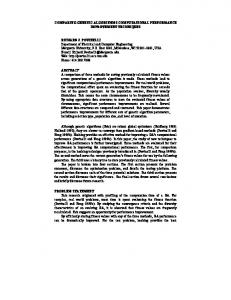
An alternative approach, pursued, e.g., by Zunger et al.,2,5,25,32,33,38 is to attempt to identify the leading interactions of Eq. 共1兲 independent of hierarchical constraints, simply by comparing the predictive power of many different CE truncations for a given alloy system. In earlier papers, this was done by fitting the numerical values of J to only a subset of the input data and then predicting the rest, an approach more recently extended to leave-many-out crossvalidation.38,72,73 The set of input structures is split into two parts, one for fitting numerical values of J, and one to check predictions made with these numerical values. The procedure is repeated for different choices of fitting or prediction sets, and the average prediction error is the cross-validation score Scv. In selective approaches, one sets up a pool of MBIT from which the leading interactions are selected without hierarchical constraints. We show in Fig. 1 some inequivalent MBIT 共beyond pairs, as pairs can be reliably accounted for by a constrained fit method5,6兲 which we use as a standard pool of MBIT candidates on the body-centered cubic 共bcc兲 lattice. Only a fraction of these MBIT are typically required, but it is not a priori clear which few must be kept. The overall pool is not designed according to any special principles. Instead, it is simply an exhaustive list of all MBIT up to a reasonable number of vertices and vertex distance, including all three-vertex MBIT up to fifth-nearest-neighbor distance, four-vertex MBIT up to fourth-nearest-neighbor distance, and five- and six-vertex MBIT up to third-nearestneighbor distance. To ensure that the relevant physics of a given alloy system is not limited by the chosen pool of MBIT, the sufficient extent of the pool can be routinely tested by including additional figures as a convergence test, e.g., all three-body figures up to eighth-nearest-neighbor distance. Figure 1 also shows that the number of possible figures increases dramatically as longer distances and more vertices are added—for instance, there are only two bcc MBIT with a maximum vertex separation of 2, but already 14 bcc MBIT with a maximum vertex separation of three. In the

FIG. 1. 共Color online兲 Pool of 45 MBIT on the bcc lattice. Figures are grouped by increasing number of vertices, and the largest vertex-vertex distance within a given figure 共2NN, …, 5NN denote second- through fifth-nearest-neighbor separation兲.

past, the relevant MBIT were selected manually from the pool by minimizing the prediction error, but an exhaustive search is not feasible; e.g., searching for only five out of a pool of 45 possible MBIT leads to as many as 1.22 million different possibilities—a task beyond a brute-force search. We have recently pointed out58 that the search for the “leading terms” of a model Hamiltonian can be efficiently performed using a genetic algorithm 共GA兲.74 In the present work, we show how this is done in particular for the choice of the MBIT which are relevant to reproduce local density approximation 共LDA兲 energies in the approach 共ii兲 above. The input information for a given alloy system is a set of first-principles calculated energies 兵EQM共␴兲其 for selected configurations ␴. The GA must then find the combination of MBIT with minimal cross-validation score, satisfying three criteria: 共1兲 It should converge significantly faster than a manual search. 共2兲 It should not get trapped in local minima. 共3兲 If there are multiple sets of MBIT which are almost equivalent to the best possible CE, the method should identify them all; a seemingly ambiguous CE for a given input set can then be unraveled by calculating selected additional input energies EQM共␴兲.

II. DETERMINISTIC CONSTRUCTION OF A MIXED-BASIS CLUSTER EXPANSION

We employ the mixed-basis cluster expansion 共MBCE兲 formalism5,6 to determine the interaction types in Eq. 共1兲, and their numerical values. Since the generality of Eq. 共1兲 is fully preserved if different configuration-dependent reference terms are added to or subtracted from the total energy of a given alloy configuration, in the MBCE one improves the

165113-3


BLUM et al.

Scv =

FIG. 2. Construction algorithm for a converged mixed-basis cluster expansion.

convergence of the cluster expansion by treating certain long-range contributions analytically.6 The MBCE-expanded energy is written as E共␴兲 = ⌬H f 共␴兲 − ECS共␴兲,

共2兲

where ⌬H f denotes the enthalpy of formation of a given, fully relaxed alloy configuration ␴ 共A1−xBx兲 from the elemental solids A and B, ⌬H f 共␴兲 = Etot共␴ ;A1−xBx兲 − 共1 − x兲Etot共A兲 − xEtot共B兲共3兲共all total energies are per atom兲. ECS共␴兲 is the configurationdependent “constituent strain energy”,6 which can be calculated analytically from LDA data, and which removes a singularity from the Fourier transform of the real-space pair interactions, J共k兲. Without subtracting ECS, this singularity would arise because ⌬H f of a fully phase-separated configuration 关A1−xBx兴phs on the same coherent underlying lattice is nonzero: Etot共关A1−xBx兴phs兲 ⫽ 共1 − x兲Etot共A兲 − xEtot共B兲, since the lattices of elemental A and B may relax independently while the coherent phase-separated limit remains constrained. The construction of a verifiably predictive cluster expansion for E共␴兲 consists of two iterative loops, as visualized in Fig. 2. The inner loop identifies the most predictive set of interaction types to describe a given set of first-principles calculated energies 兵ELDA共␴兲其 for Ns input structures. The measure for the predictive power of a given set of interaction types is a leave-many-out cross-validation score72,73 Scv, as defined in Ref. 38. The Ns input structures are subdivided into a group of N f ⬍ Ns structures to fit the numerical values of the selected interaction types, and a group of Nv = Ns − N f structures which are not fitted, so that their predicted energies ECE共␴兲 can be compared to the known energy ELDA共␴兲 after the fit. This process is then repeated for b independent subdivisions into N f fitting and Nv prediction structures, until each of the Ns input energies 兵ELDA共␴兲其 was predicted at least twice. The average overall prediction errors from this process define

1 兺 bNv 共b sets兲共Nv

兩ECE共␴兲 − ELDA共␴兲兩2 . 兺 ␴ in set兲

共4兲

The goal of the inner loop, then, is to identify the combination共s兲 of interaction types 共candidate CEs兲 with minimal Scv. The outer loop acts as a feedback loop to ensure that a CE, identified in the inner loop for the fixed subset of NS structures, really possesses good predictive power for all 2N configurations. Each candidate CE is used to search all 2N structures for additional ground states or near-ground-state structures ␴new. Their energies ELDA共␴new兲 are then evaluated by direct LDA calculations and compared to the predicted ECE共␴new兲, giving an objective estimate of the predictive power of each candidate cluster expansion. The newly calculated 兵ELDA共␴new兲其 are added to the previous input set, and the inner loop is repeated. The outer loop iterations are converged when no more significant new ground-state structures are predicted, and all verified predicted energies agree with their direct LDA counterparts to within a few meV. For bulk alloys, ⲏ50 LDA input structures38,59 are usually enough to achieve convergence. The complete iterative procedure guarantees the identification of a well-converged truncated expansion Eq. 共1兲, and additionally acts as a prediction engine for important candidate structures for ground states whose energy must be calculated directly in LDA. The inner loop is where the difficult search problem for the most relevant interaction types arises, as outlined in the introduction. This problem is manageable for pairs, whose number increases relatively slowly with distance, and which can therefore be treated by the constrained fit method of Ref. 6, but the number of MBIT with three or more vertices increases much more rapidly with distance. The present paper concentrates on the selection of MBIT. We thus assume a fixed set of input structures, and always use the constrained fit method for pair interactions. Our goal is to select the best set of MBIT to minimize Scv using a genetic algorithm. The rest of the paper explains how this task is done. III. GENETIC ALGORITHM SELECTION OF MBIT

Genetic algorithms74 use the biological idea of “survival of the fittest” to find the optimum solution to a given problem. GA’s are particularly helpful when faced with strongly correlated search spaces, where other algorithms such as the sequential optimization of individual parameters, or methods based on individual, random parameter “flips” 共Monte Carlo兲 would end up in local minima, or even fail to converge at all. GA’s have been applied in many different settings, e.g., in computational condensed matter physics to find the optimal numerical values of given physical parameters such as geometric structure75–78 or tight-binding parameters.79 Our present application is different in that we aim to find the actual shape of a cluster expansion Hamiltonian, i.e., its interaction types rather than only their numerical values. Generally, the trial solutions in a GA are encoded as binary sequences 共the “genomes”兲 of 0’s and 1’s 共the “genes”兲. Here, the objective is to pick, from a large pool, a handful5–10 of MBIT to be included in a trial CE, i.e., a truncation of Eq. 共1兲. A natural encoding of trial CE is a

165113-4



genome “…01110100011…” with one gene for each candidate MBIT in the pool, and a one 共zero兲 denoting whether that figure is 共is not兲 included. Over the course of the GA, a set of genomes is monitored over many iterations 共“generations”兲. From one iteration to the next, “child” genomes are created by a cross-over 共“mating”兲 of two selected “parent” genomes of the earlier iteration. Each gene of a child genome takes on the value of that gene in either the first or the second parent. If this strategy were strictly implemented, only preexisting “genetic” information could be proliferated in a mating step. So, if a certain MBIT 共or combination兲 were eliminated from the entire population of trial CE’s in any one generation, this MBIT could never return later. A GA might lose a vital piece of the optimal solution at an early stage by accident and would later be doomed to remain stuck in a local 共but not global兲 optimum forever. Nature’s solution to this dilemma is mutation. To prevent a starvation of the diversity of possible trial solutions, individual genes can randomly be turned on or off in a newly created child genome, similar to the random mutations of evolutionary biology. We make the following choices 关Sec. III A–III F below兴 to control the convergence of our particular GA. A. Maximum number of “active” genes per genome

The “genomes” in our problem represent sets of MBIT 共i.e., figure types as opposed to numerical values J兲 which are used to construct a CE. The optimized quantity is the cross-validation score Scv, which measures the ability of a given CE to predict EQM for structures not used in the fit. One additional measure is taken as a safeguard against overoptimization of Scv: we impose a deliberate limit on the number NMB of active MBIT per CE, i.e., we cap the number of active genes 共“ones”兲 in each genome. The development of Scv as a function of NMB may be studied to determine to what degree an increase in the number of CE parameters still helps improve predictive accuracy significantly. B. Population size

The number of genomes per generation, Npop, determines the amount of “genetic diversity” which is available to spawn subsequent generations. For optimum genetic diversity, we choose Npop based on the number of MBIT in each CE, NMB, with the requirement that each MBIT appear at least twice 共possibly more often兲 in the initial generation.

and ones兲 of the child genome are selected from parent 1 or parent 2. The parent with better fitness has a higher probability of passing its genes on to the child than the less fit parent. In this way, the preferred proliferation of “better” genetic information is ensured. E. Mutation rate

After each mating step, we allow each gene to be “flipped” from zero to one or vice versa with a certain 共relatively low兲 probability. In fact, we choose this probability so as to obtain a certain number of flips Nflips per genome on average. Of course, we might accidentally end up with more MBIT in a CE than allowed by the maximum number NMB after this step. In that case, we randomly pick some of these “ones” and turn them off 关i.e., we remove figures from the corresponding truncation of Eq. 共1兲兴, until their number is reduced to the prescribed target number. F. “Lock-out” strategy

Even with significant initial genetic diversity and mutations, the problem of local optima—which exists in any global optimization scheme, not just a GA—is not fully resolved. If the GA first reaches a locally optimal CE that differs from the global one by several MBIT, the probability to progress by random mutations alone may become hopelessly small. As a result, the prospective alloy researcher may easily spend thousands of generations waiting for the correct minimum to be found. Even worse, in an actual application the best answer is not known, and hence it is impossible to be sure whether or not a persistent solution is already the best possible CE or not. To overcome this “locking” of the algorithm into a local minimum, we implement the idea of “locking out” any persistent solutions after progress has stopped for a certain number of generations 共50–100兲. The persistent CE is recorded on a blacklist, and barred from ever occurring again. The algorithm is then reinitialized with a momentarily increased mutation rate in the next generation. The benefit is twofold. First, the algorithm is forced to look for another CE, which may or may not be better than the first. Second, the result of a GA run is a list of several nearoptimal CEs in addition to the actual optimum. This gives direct insight into the degree of degeneracy of the search space explored. IV. APPLICATION TO MO-TA

C. Survival rate

A fraction rs of the original Npop candidate genomes with the momentary optimum fitness is retained from one generation to the next. The other genomes are replaced with children mated from the preceding generation. For instance, from a generation of 20 genomes with a survival rate rs = 1 / 2, the ten best individuals would be carried over unmodified. Ten children would be created to fill the remaining slots. D. Mating favoritism

To create a child, two parents are randomly selected from the existing generation. Then, one by one the genes 共zeroes

The criteria Sec. III A–III F determine our algorithm completely. Once the key parameters are set, the mating process can be repeated for an arbitrary number of generations until a target value of Scv has been achieved. A. Successful retrieval of the leading interactions

We first demonstrate the GA’s ability to successfully retrieve the leading interactions from an input set 兵Eexact共␴兲其 whose underlying interactions are exactly known. To that end, we use Eq. 共1兲 itself to calculate Eexact共␴兲 for 60 bcc input configurations ␴, inserting the set interactions retrieved

165113-5


BLUM et al.

FIG. 3. Identification of the five optimum MBIT out of a pool of 45 for the input set 兵Eexact共␴兲其. 共a兲 Development of Scv as a function of GA generation number for all trial CEs. Persistent solutions are locked out after 50 generations. The optimum combination of MBIT is locked out in generation 97. 共b兲 List of the first six locked-out “persistent” CEs, encoded as genomes.

in an earlier study of the alloy system Mo-Ta.37,38 共for details see Appendix A兲. This choice is advantageous because the underlying cluster expansion describes a real alloy system. In Refs. 37 and 38, the cluster expansion was constructed manually and tested thoroughly, predicting physical ground states, order-disorder transition temperatures Tc, short-range order, and the random alloy enthalpy of mixing of Mo-Ta. Figure 3共a兲 shows the development of Scv as a function of generation number in a typical GA run. The GA picks the optimum five MBIT out of a pool of 45 candidates 共Fig. 1兲, using Npop = 27 trial CEs to truncate Eq. 共1兲. The 13 fittest CEs of each generation are allowed to survive into the next generation. The mutation rate is chosen to flip one gene per newly mated child on average, meaning that the mutation probability is 1 / 45 to switch a particular MBIT off or on at random. Since the input energies Eexact共␴兲 are constructed from the known interactions of Table I, the search must select these precise MBIT, with Scv = 0. This optimum solution is indeed obtained after 46 generations. To arrive at this result, only 657 individual combinations of MBIT were probed, less than 1 / 1000 of the total space which contains of 共 455 兲 ⬇ 1.22 million distinct possible CEs. After the optimum CE is identified, it persists through the subsequent iterations of the GA, and is therefore “locked out” after 96 generations. The algorithm then continues to probe the search space for a next best CE, and so forth. Figure 3共b兲 lists the six CE’s which were locked out within 600 GA generations of this run. All six candidates share two specific MBIT, but differ in the remaining three. In terms of Scv, the best solution is clearly separated from the competing possible truncations of Eq. 共1兲. It is noteworthy that for the selected lock-out criterion 共exclude persistent solutions after

TABLE I. Interaction types and 共symmetry-weighted兲 numerical interaction values for bcc Mo-Ta according to Refs. 37 and 38, used here to generate the set of configurational energies 兵Eexact共␴兲其. Figure

165113-6

Vertices 关excl. 共0,0,0兲兴

Numerical value 共meV兲

Empty and point interaction J0 J1

−144.7 +12.8 Pair interactions

1 2 3 4 5 6 7 8

共0.5,0.5,0.5兲共1,0,0兲共1,1,0兲共1.5,0.5,0.5兲共1,1,1兲共2,0,0兲共1.5,1.5,0.5兲共2,1,0兲

+108.1 −15.7 +23.0 −3.7 +12.0 +3.7 +6.3 +21.2

Three-body interactions M1 M2 M3 M4

共0.5,0.5,0.5兲, 共1,1,0兲共0.5,0.5,0.5兲, 共1.5,0.5,0.5兲共0,1,1兲,共1.5,0.5,0.5兲共1,0,0兲,共1,1,1兲

−3.7 −21.8 −5.2 +18.1

Four-body interactions M5

共0.5,0.5,0.5兲,共1,1,0兲, 共1.5,0.5,0.5兲

−9.8



FIG. 4. Identification of the five optimum MBIT out of a pool of 45 for 兵ELDA共␴兲其 of bcc Mo -Ta. 共a兲 Development of Scv of all trial solutions as a function of GA generation number. Persistent solutions are locked out after 50 generations. The optimum CE is found second, in generation 209, after a persistent local minimum has been removed. 共b兲 List of the first eight locked-out “persistent” CEs, encoded as genomes.

50 generations兲, the six optimum CE’s are not found precisely in order of increasing Scv. Without locking out, the third and fourth identified CEs 共in generations 264 and 350兲 could have significantly delayed the algorithm’s convergence to the actual third-best solution 共Scv = 1.09 meV, locked out in generation 443兲. Next, we show that the GA performs just as well for actual LDA input data for Mo-Ta. The input set 兵ELDA共␴兲其

consists of the 56 structures used in Refs. 37 and 38, and is described in Appendix B. To construct the optimum CE for 兵ELDA共␴兲其, we again pick the five MBIT out of the pool of 45 candidates 共Fig. 1兲, using the same basic GA settings as for 兵Eexact共␴兲其. The GA run shown in Fig. 4共a兲 demonstrates a case where the algorithm is first trapped in a local minimum, which is then locked out after 96 generations total 共50 generations after it first appears兲 according to criterion in Sec. III

FIG. 5. Number of trial CEs evaluated by the GA as a function of 共a兲 population size of each generation, 共b兲 survival rate between two generations, and 共c兲 mutation rate in the mating step. Ten different GA runs were evaluated in each step 共open symbols兲. The full line represents the average number trial solutions for each setting of GA parameters, including their standard deviation 共error bars兲. 165113-7


BLUM et al.

FIG. 6. 共a兲 Number of trial CEs evaluated by the GA as a function of mutation rate in the mating step to find the optimum five MBIT for 兵ELDA共␴兲其. All settings are the same as for Fig. 5共c兲. 共b兲 Same input data and parameters, except persistent candidate CEs are now locked out after 50 generations without improvement.

F above. 共That these numbers are the same as for the first lock-out in Fig. 3 is pure coincidence.兲 The actual optimum solution is found second, after 159 generations, and locked out in generation 209. Compared to the total space of 共 45 5 兲 ⬇ 1.22 million possibilities, again only ⬇1 / 1000 of the solution space was explored. Figure 4共b兲 shows the list of locked-out trial CEs after 600 generations. Since, for actual LDA input data, there is no exact solution, the optimum selected individuals are much closer together in terms of Scv than in the case of 兵Eexact共␴兲其共Fig. 3兲. Still, the best solution is relatively clearly separated from the competing possible CEs. Indeed, it coincides with the result of our previous, much more tedious search “by hand”38 共Table I兲, yet this time with certainty that no correlations between the MBIT are missed. All further locked-out CEs share three of the optimum MBIT. It is instructive to note that the nonoptimal solution which was locked out first differs from the actual optimum in both remaining MBIT. Its relative persistence is thus explained by the lower probability of a correlated switch of two MBIT, required to reach the actual best solution.

larger symbols including lines and error bars. It is obvious that the scatter of results is relatively large, but several trends are nevertheless apparent. 共a兲 The effect of population size. We use a probability of one mutation on average per newly mated child and rs = 1 / 2. The impact of Npop on the overall computational effort of our algorithm is relatively small. As we increase Npop, the number of new trial CEs per generation increases. However, the average number of generations needed to find the actual

B. Optimizing the algorithm’s efficiency

We examine the impact of the three major scalable parameters, population size, survival rate, and mutation rate, on the convergence efficiency of our algorithm. This first set of tests is based on the input set 兵Eexact共␴兲其 as described in Appendix A. For clarity, the lock-out criterion was not applied when generating these results. Figures 5共a兲–5共c兲 show the performance of the GA as a function of 共a兲 population size Npop, 共b兲 survival rate rs, and 共c兲 mutation rate in the mating step. As we aim to visualize the actual computational effort, we plot the total number of trial CEs that the GA explored before the solution was found, i.e., the number of child CEs per generation Npop ⫻ rs multiplied by the number of generations needed to find the correct solution. For each choice of parameters, ten different GA runs were evaluated, shown as small open circles. Also plotted are their averages and standard deviations, represented by

FIG. 7. Configurational heat capacity Cv共T兲 from Monte Carlo simulations of the A2-B2 phase transition in Mo0.5Ta0.5 by stepwise cooling. Cv共T兲 is shown for the optimum CE selected in Fig. 4共b兲, three near-optimal CE candidates, and an ad hoc hierarchy-based expansion which contains the five shortest-ranged MBIT of Fig. 1.

165113-8



solution decreases almost as fast with Npop, leaving the total number of required trial CEs almost constant. So, while it seems slightly beneficial to sample fewer rather than more new trial solutions per generation, the overall effect is not dramatic. 共b兲 The effect of the survival rate. We set a probability of one mutation on average per newly mated child, and Npop = 27. The scatter of results is again larger than any actual trend, but it does seem that high survival rates 共down to only one newly created CE per generation兲 give somewhat better results. The GA then makes the most efficient use of the previously acquired genetic information, since each child is generated almost exclusively from previously accepted survivors, rather than from a parent which was itself a child in the preceding generation, with potentially high Scv. 共c兲 The effect of the mutation rate. This governs the childmating process, and shows the clearly strongest effect of all the adjustable quantities. Tested for Npop = 27 and rs = 13/ 27, a logarithmic plot is needed to display the full results. It is evident that the fastest results are reached for 0.5–2 mutations per mating step. Lower mutation rates slow down the algorithm because not enough fresh genetic information is introduced, causing the algorithm to dwell in local minima over many generations. In contrast, mutation rates that are too high lead to an almost random search pattern, drowning out the useful information that the algorithm has already collected in preceding search generations. For the simple test case only around 1 / 1000 of the available search space must be scanned to find the best possible CE. While the algorithm does not fail for any of the tested settings, an appropriate mutation rate is the key to its efficient functioning. C. Impact of the lock-out criterion

Figure 6 shows the performance 共number of trial CEs required to find the actual optimum set of MBIT, as previously

determined in a tedious search by hand38兲 of the GA as a function of mutation rate for actual LDA data 兵ELDA共␴兲其 of Mo-Ta 共Appendix B兲. In Fig. 6共a兲, all settings are exactly the same as for Fig. 5共c兲; in particular, persistent solutions were never locked out. Again, we averaged over ten GA runs for each setting, and also show the scatter of individual runs. The scatter of the number of required trial CE evaluations is much larger for 兵ELDA共␴兲其 than for 兵Eexact共␴兲其 in Fig. 5共c兲. Moreover, a minimum develops only at two mutations per child genome on average, which appears as a sharp spike. The reason for this behavior can also be seen in Fig. 6共a兲. A number of individual test runs shows exactly the same behavior as observed for 兵Eexact共␴兲其 in Fig. 5共c兲, namely a parabolalike distribution with a minimum around 0.5–2 mutations per genome. However, another group of runs takes disproportionately longer 共data points between 10 000 and 100 000 trial solutions兲, driving up both the average and the standard deviation of our search. The origin of this population of outliers is that, in these cases, the GA encounters a local optimum CE that differs by several MBIT from the actual one. The actual optimum can now only be reached by several random mutations in the same step, which must all be simultaneously correct. The probability for this correlated switch is low, and the algorithm remains trapped for some time. This problem is particularly grave for small mutation rates, where a large number of test runs do not find the correct CE at all within 5000 generations, as shown by the success rate in the upper panel of Fig. 6共a兲. This behavior is mended by the “lock-out” strategy described in the preceding section. In Fig. 6共b兲, the lock-out threshold is set to 50 generations, with otherwise the same parameters as Fig. 6共a兲. The success of this strategy is convincing; the outlier population is eliminated entirely, and the qualitative behavior is now the same as that of Fig. 5. In particular, the success rate is now 100% even in the previously difficult cases of very low mutation rates. It is also worth noting that the lock-out strategy does not improve the

FIG. 8. Physical data E共␴兲 as a function of composition x of each configuration ␴, based on which the GA selects the optimum MBIT in the present work. Dashed lines serve as guides to the eye. 共a兲 Eexact共␴兲 for 60 bcc configurations, calculated directly from Eq. 共1兲 using the interaction parameters tabulated in Table I. 共b兲 LDA-calculated input set ELDA共␴兲 = ⌬HLDA共␴兲 − ECS共␴兲 for 56 configurations of bcc Mo-Ta. 165113-9


BLUM et al.

TABLE II. Eexact共␴兲 for 60 input configurations, generated from Eq. 共1兲 using the interactions of Table I. See text for details of the structure notation used. Composition Mo Mo11Ta Mo9Ta Mo8Ta Mo6Ta Mo5Ta Mo4Ta

Mo3Ta

Mo8Ta3 Mo5Ta2 Mo2Ta

Mo5Ta3 Mo3Ta2 Mo4Ta3 MoTa

Structure A2 共211兲 A11B SL 共521兲 A9B SL “A8B” 共111兲 A6B SL 共332兲 A5B SL 共100兲 A4B SL 共310兲 A4B SL 共332兲 A6BA2B D03 L60 共100兲 A3B SL 共110兲 A3B SL “A4B12” SQS-16 共111兲共A3B兲2A2B SL 共111兲 A5B2 SL C11b 共110兲 A2B SL 共111兲 A2B SL “A5B3” 共100兲 A2BAB SL 共111兲 A2BAB SL 共111兲 A2B共AB兲2 SL SQS-14 A1 B2 B11 B32 共110兲 A2B2 SL

E共␴兲共meV兲 0.9 −46.1 −55.6 −66.8 −81.9 −93.2 −120.8 −113.0 −115.5 −139.9 −136.8 −143.0 −92.2 −146.2 −111.7 −140.4 −102.4 −192.4 −117.1 −133.8 −137.2 −210.8 −195.8 −211.8 −148.9 −135.2 −221.9 −162.1 −125.6 −104.7

Composition

Structure

E共␴兲共meV兲

MoTa

共310兲 A2B2 SL 共311兲 A3B3 SL 共221兲 A4B3A2B3 SL 共221兲 A3B2A3B4 SL SQS-16 共111兲 A2B共AB兲2 SL SQS-14 共100兲 A2BAB SL 共111兲 A2BAB “A5B3” C11b 共110兲 A − 2B SL 共111兲 A2B SL 共111兲 A5B2 SL 共111兲共A3B兲2A2B SL D03 L60 共100兲 A3B SL 共110兲 A3B SL “A4B12” SQS-16 共100兲 A4B SL 共310兲 A4B SL 共332兲 A6BA2B 共332兲 A5B SL 共111兲 A6B SL “A8B” 共521兲 A9B SL 共211兲 A11B SL A2

−211.7 −218.4 −120.4 −127.7 −144.3 −203.4 −143.9 −201.3 −191.3 −128.4 −176.5 −100.5 −124.3 −87.8 −109.3 −96.2 −95.7 −116.4 −79.7 −139.5 −105.8 −99.6 −111.8 −106.1 −76.9 −62.0 −56.5 −49.6 −39.3 1.1

Mo3Ta4 Mo2Ta3 Mo3Ta5 MoTa2

Mo2Ta5 Mo3Ta8 MoTa3

MoTa4

MoTa5 MoTa6 MoTa8 MoTa9 MoTa11 Ta

behavior for unreasonably high mutation rates 关e.g., 10 mutations per genome in Fig. 6共b兲兴. Here, the convergence is slowed down not by trapping in local minima but by the noise of random mutations drowning out the valuable genetic information—the lock-out solution does not apply. For reasonable mutation rates, the algorithm is now completely reliable. V. PHYSICAL IMPACT

We have shown how a GA can be employed to solve a decisive step in the construction of a CE Hamiltonian of the form Eq. 共1兲. Based on a set of sufficiently many configurational energies 兵E共␴兲其, identify those interaction types which promise the greatest power to predict energies of further, as yet unknown energies for the same alloy system. During the construction process of a CE, one may test predictions made with these MBIT after the fact, and increase the number of structures ␴ for which first-principles input is available. A

completed CE then provides the ability to assess the energies of literally millions of configurations within minutes, enabling both the identification of ground-state structures by exhaustive search,25 and the evaluation of configurational averages, e.g., in Monte Carlo simulations,26,27 for finite-T thermodynamics. In addition, the rigorous application of the lock-out criterion provides physical information beyond that contained in the optimum set of MBIT alone. With a rigorous list of nearoptimal cluster expansions, it is now possible to assess how sensitive the physical target quantities of a cluster expansion are against the final choice of MBIT, i.e., how reliable the information is that we can extract from a given set of input structures 兵␴其input. As an example, we examine the A2-B2 phase transition in bcc Mo0.5Ta0.5 using canonical Monte Carlo simulations 共cell size: 16⫻ 16⫻ 16, 4000 flips per lattice site and T step兲. Figure 7 shows the development of the configurational heat capacity Cv with decreasing simulation temperature for the optimum selected set of MBIT in Fig.

165113-10



TABLE III. Full input set 兵ELDA共␴兲其关Eq. 共2兲兴 for 56 bcc Mo-Ta input configurations. See Ref. 38 for details. Composition Mo Mo8Ta Mo7Ta Mo6Ta Mo5Ta Mo4Ta

Mo3Ta

Mo5Ta2 Mo2Ta

Mo9Ta5 Mo5Ta3 Mo3Ta2

Mo4Ta3

Structure

E共␴兲共meV兲

Composition

Structure

E共␴兲共meV兲

A2 “A8B” 共210兲 A7B SL “A7B” 共100兲 A6B SL 共111兲 A6B SL 共433兲 A8BA2B SL 共111兲 A4B SL 共100兲 A4B SL 共310兲 A4B SL D03 L60 共100兲 A3B SL 共110兲 A3B SL 共310兲 A3B SL “A12B4-I” “A4B12” “A12B4-II” 共100兲 A3BA2B SL 共111兲 A4BAB SL C11b 共110兲 A2B SL 共111兲 A2B SL 共710兲 A4B3A4BAB SL 共210兲 A3B共AB兲2 SL 共210兲 A3B共AB兲3 SL 共111兲 A2BAB SL 共100兲 A2BAB SL 共100兲 A2B共AB兲2 SL 共111兲 A2B共AB兲2 SL

0.0 −69.2 −69.8 −71.9 −84.9 −81.6 −94.8 −112.9 −120.4 −116.9 −140.3 −140.8 −145.8 −90.0 −144.1 −137.8 −142.6 −139.7 −163.3 −161.6 −193.1 −116.2 −134.1 −190.4 −195.9 −197.8 −193.6 −211.3 −212.4 −210.4

MoTa

A1 B2 B11 B32 共110兲 A2B2 SL 共310兲 A2B2 SL “A8B8” 共100兲 A2B共AB兲2 SL 共111兲 A2B共AB兲2 SL 共100兲 A2BAB SL C11b 共110兲 AB2 SL 共111兲 AB2 SL “A4B9” D03 L60 共100兲 AB3 SL 共110兲 AB3 SL 共310兲 AB3 SL “A4B12” “A12B4-II” 共100兲 A4B SL 共310兲 A4B SL 共210兲 A7B SL “A8B” A2

−135.4 −222.4 −165.1 −127.3 −103.8 −209.8 −152.6 −201.6 −203.8 −198.0 −174.8 −103.0 −121.7 −170.1 −93.4 −94.9 −120.7 −77.9 −127.7 −140.5 −112.6 −97.6 −105.5 −60.2 −51.9 0.0

4共b兲, and the three best near-optimal candidates of Fig. 4共b兲. As a contrast, the result for an ad hoc hierarchy-based CE is also shown; this CE also contains five MBIT, but they are now the four shortest-ranged three-body interaction types and the shortest-ranged four-body interaction type of Fig. 1. As shown in Ref. 38 for the optimum CE, the A2-B2 transition occurs for Tc ⬇ 600– 1000 K. Cv共T兲 is quantitatively very similar to the optimum CE for all three near-optimal CE’s, as expected at the end of a well-converged CE construction process, which is based on a large enough input database 兵␴其input. In contrast, Cv共T兲 from the shorter-ranged ad hoc CE differs clearly from the other four curves, and would falsely suggest a clearly higher Tc than all others, close to 1000 K. However, this ad hoc CE is safely ruled out by the GA, since it is characterized by Scv ⬇ 7.0 meV, more than twice the prediction error estimated for the GAdetermined near-optimal MBIT combinations.

Mo3Ta4 Mo2Ta3 MoTa2

Mo4Ta9 MoTa3

MoTa4 MoTa7 MoTa8 Ta

VI. CONCLUSION

We show how a genetic algorithm removes most human guesswork from the construction of a cluster expansion, where otherwise a select few combinations of MBIT 共e.g., the shortest兲 would have to be favored over millions of other possible combinations by some intuition. The algorithm converges fast both for the test case where the correct solution is known analytically, and for realistic first-principles input data to a cluster expansion. The algorithm is easy to use, since its performance is almost exclusively controlled by the mutation rate alone, and it is robust against getting stuck in apparent local optima by strictly “locking out” persistent solutions. The resulting list of near-optimal solutions can be used to verify directly the reliability of all CE-predicted physical alloy properties 共ground states, phase transitions, short-range order兲. The procedure is not restricted to the cluster expansion method which we emphasize here, and we

165113-11


BLUM et al.

expect the same benefits in the construction of any general model Hamiltonian where a system-dependent choice of parameter types must be made. ACKNOWLEDGMENTS

The following support is gratefully acknowledged: NREL financial support by contract DOE-SC-BES-DMS; M.J.W. and G.L.W.H. supported through the Intramural Grant Program at Northern Arizona, and the NSF through DMR0224183. M.J.W. is also grateful for partial funding from Research Corporation, CC5944. APPENDIX A: INPUT SET Êexact„␴…‰ FOR MA-TA: CONFIGURATIONS AND ENERGIES

configurations include the bcc configurations of elemental Mo and Ta, the “usual suspect” configurations B2 MoTa, B32 Mo2Ta2, D03 Mo3Ta and MoTa3, and C11b Mo2Ta and MoTa2, as well as 14 other structures with four or fewer atoms per unit cell, and five special quasirandom structures with 14 or 16 atoms per unit cell 共as described in the appendix of Ref. 38兲. The remaining 33 structures are all relatively low in energy, spanning unit cell sizes between 5 and 16 atoms across a broad range of intermediate concentration values; a full listing is given in Table II. Wherever possible, the structures are described in a short way as superlattices 共SLs兲 of pure atomic planes 共e.g., the “共100兲 A2BAB SL” is a sequence of two pure 共100兲 planes of element A, followed by one pure B plane, another A and another B plane兲. Where such a notation is not possible, a description of the structure is referred to Ref. 38. There is one structure which neither fits a superlattice notation nor has been described previously—this is the structure labeled “A5B3.” It is a sequence of three mixed 共100兲 planes of c共2 ⫻ 2兲 type AB occupation, followed by one plane of pure A.

To test our algorithm using an input database for which an exact solution is known, we selected 60 bcc-based configurations ␴. We calculated 兵Eexact共␴兲其 for each ␴ according to Eq. 共1兲 using the interactions of Table I, which were found to describe the Mo-Ta alloy system in Refs. 37 and 38. It is evident that the MBIT do not follow from a simple scheme of selection among the 45 interactions displayed in Fig. 1: they include four three-body-figures, one of them extending to the fifth-nearest-neighbor vertex 共1,1,1兲, and one fourbody figure with a fourth-nearest-neighbor vertex 共1.5,0.5,0.5兲. In a hierarchy-based approach, this choice would mandate a large number of additional unrelated figures. The distribution of 兵Eexact共␴兲其 is shown in Fig. 8共a兲 as a function of the atomic concentration x of each configuration ␴. There is some energetic asymmetry with regard to equiatomic composition, with lower E共␴兲 towards the Mo-rich side, and it is precisely this asymmetry which is captured by three-body MBIT 共pair interactions alone would produce a symmetric distribution of configurations兲. The chosen input

A description of all Mo-Ta input structures ␴ and a listing of their formation enthalpies ⌬HLDA共␴兲 can be found in Ref. 38. In the application of the GA above, we do not use ⌬HLDA共␴兲 directly, but rather ELDA共␴兲 = ⌬HLDA共␴兲 − ECS共␴兲关Eq. 共2兲兴. ECS共␴兲 denotes the constituent strain energy, calculated according to Eq. 共5兲 and Fig. 5 of Ref. 38. We tabulate ELDA共␴兲 for all 56 Mo-Ta input structures in Table III. ELDA共␴兲 as a function of a configuration’s concentration x is also displayed in Fig. 8共b兲.

*Present address: Abteilung Theorie, Fritz-Haber-Institut der

10 R.

Max-Planck-Gesellschaft, Faradayweg 4-6, 14195 Berlin-Dahlem, Germany. 1 J. M. Sanchez, F. Ducastelle, and D Gratias, Physica A 128, 334 共1984兲. 2 A. Zunger, Statics and Dynamics of Alloy Phase Transformations, edited by P. E. A. Turchi and A. Gonis 共Plenum Press, New York, 1994兲, pp. 361–419. 3 D de Fontaine, Solid State Phys. 47, 33 共1994兲. 4 A. van de Walle and G. Ceder, J. Phase Equilib. 23, 348 共2002兲. 5 A. Zunger, L. G. Wang, G. L. W. Hart, and M. Sanati, Modell. Simul. Mater. Sci. Eng. 10, 685 共2002兲. 6 D. B. Laks, L. G. Ferreira, S. Froyen, and A. Zunger, Phys. Rev. B 46, 12587 共1992兲. 7 M. H. F. Sluiter, K. Esfarjani, and Y. Kawazoe, Phys. Rev. Lett. 75, 3142 共1995兲. 8 C. Berne, M. Sluiter, Y. Kawazoe, T. Hansen, and A. Pasturel, Phys. Rev. B 64, 144103 共2001兲. 9 C. Berne, M. Sluiter, Y. Kawazoe, and A. Pasturel, J. Phys.: Condens. Matter 13, 9433 共2001兲.

APPENDIX B: INPUT SET ÊLDA„␴…‰ FOR MO-TA: CONFIGURATIONS AND ENERGIES

Osório, S. Froyen, and A. Zunger, Phys. Rev. B 43, 14055 共1991兲. 11 R. Osório, S. Froyen, and A. Zunger, Solid State Commun. 78, 249 共1991兲. 12 R. Osório, Z.-W. Lu, S.-H. Wei, and A. Zunger, Phys. Rev. B 47, 9985 共1993兲. 13 C. Wolverton and D. de Fontaine, Phys. Rev. B 49, 8627 共1994兲. 14 G. Rubin and A. Finel, J. Phys.: Condens. Matter 7, 3139 共1995兲. 15 R. McCormack and D. de Fontaine, Phys. Rev. B 54, 9746 共1996兲. 16 R. Osório, J. E. Bernard, S. Froyen, and A. Zunger, Phys. Rev. B 45, 11173 共1992兲. 17 S. Froyen, J. E. Bernard, R. Osório, and A. Zunger, Phys. Scr., T T45, 272 共1992兲. 18 R. Drautz, H. Reichert, M. Fähnle, H. Dosch, and J. M. Sanchez, Phys. Rev. Lett. 87, 236102 共2001兲. 19 R. Drautz, R. Singer, and M. Fähnle, Phys. Rev. B 67, 035418 共2003兲. 20 M. H. F. Sluiter and Y. Kawazoe, Phys. Rev. B 68, 085410 共2003兲.

165113-12


USING GENETIC ALGORITHMS TO MAP FIRST-… Müller, J. Phys.: Condens. Matter 15, R1429 共2003兲. R. Singer, R. Drautz, and M. Fähnle, Surf. Sci. 559, 241 共2004兲. 23 H. R. Tang, A. van der Ven, and B. L. Trout, Mol. Phys. 102, 273 共2004兲. 24 H. Tang, A. Van der Ven, and B. L. Trout, Phys. Rev. B 70, 045420 共2004兲. 25 L. Ferreira, S.-H. Wei, and A. Zunger, Int. J. Supercomput. Appl. 5, 34 共1991兲. 26 Z. W. Lu, D. B. Laks, S.-H. Wei, and A. Zunger, Phys. Rev. B 50, 6642 共1994兲. 27 A. van de Walle and M. Asta, Modell. Simul. Mater. Sci. Eng. 10, 521 共2002兲. 28 S.-H. Wei, A. A. Mbaye, L. G. Ferreira, and A. Zunger, Phys. Rev. B 36, 4163 共1987兲. 29 J. E. Bernard, L. G. Ferreira, S.-H. Wei, and A. Zunger, Phys. Rev. B 38, 6338 共1988兲. 30 S.-H. Wei, L. G. Ferreira, and A. Zunger, Phys. Rev. B 41, 8240 共1990兲. 31 S.-H. Wei, L. G. Ferreira, and A. Zunger, Phys. Rev. B 45, 2533 共1992兲. 32 V. Ozolins, C. Wolverton, and A. Zunger, Phys. Rev. B 57, 6427 共1998兲. 33 S. Müller, L.-W. Wang, A. Zunger, and C. Wolverton, Phys. Rev. B 60, 16448 共1999兲. 34 G. L. W. Hart and A. Zunger, Phys. Rev. Lett. 87, 275505 共2001兲. 35 S. Müller and A. Zunger, Phys. Rev. B 63, 094204 共2001兲. 36 M. Sanati, G. L. W. Hart, and A. Zunger, Phys. Rev. B 68, 155210 共2003兲. 37 V. Blum and A. Zunger, Phys. Rev. B 69, 020103共R兲共2004兲. 38 V. Blum and A. Zunger, Phys. Rev. B 70, 155108 共2004兲. 39 L. G. Ferreira, A. A. Mbaye, and A. Zunger, Phys. Rev. B 37, 10547 共1988兲. 40 L. G. Ferreira, S.-H. Wei, and A. Zunger, Phys. Rev. B 40, 3197 共1989兲. 41 J. W. D. Connolly and A. R. Williams, Phys. Rev. B 27, R5169 共1983兲. 42 F. Ducastelle and F. Gautier, J. Phys. F: Met. Phys. 6, 2039 共1976兲. 43 S. de Gironcoli, P. Giannozzi, and S. Baroni, Phys. Rev. Lett. 66, 2116 共1991兲. 44 J. B. Staunton, D. D. Johnson, and F. J. Pinski, Phys. Rev. B 50, 1450 共1994兲. 45 A. V. Ruban, S. Shallcross, S. I. Simak, and H. L. Skriver, Phys. Rev. B 70, 125115 共2004兲. 46 R. Drautz, M. Fähnle, and J. M. Sanchez, J. Phys.: Condens. Matter 16, 3843 共2004兲. 47 N. Marzari, S. de Gironcoli, and S. Baroni, Phys. Rev. Lett. 72, 4001 共1994兲. 48 A. Gonis, X.-G. Zhang, A. J. Freeman, P. Turchi, G. M. Stocks, and D. M. Nicholson, Phys. Rev. B 36, 4630 共1987兲. 49 A. V. Ruban and H. L. Skriver, Phys. Rev. B 66, 024201 共2002兲. 50 A. V. Ruban, S. I. Simak, P. A. Korzhavyi, and H. L. Skriver, 21 S. 22

Phys. Rev. B 66, 024202 共2002兲. F. J. Pinski, J. B. Staunton, and D. D. Johnson, Phys. Rev. B 57, 15177 共1998兲. 52 R. Magri, S.-H. Wei, and A. Zunger, Phys. Rev. B 42, 11388 共1990兲. 53 A. V. Ruban, S. I. Simak, S. Shallcross, and H. L. Skriver, Phys. Rev. B 67, 214302 共2003兲. 54 R. Monnier, Philos. Mag. B 75, 67 共1997兲. 55 D. D. Johnson, A. V. Smirnov, J. B. Staunton, F. J. Pinski, and W. A. Shelton, Phys. Rev. B 62, R11917 共2000兲. 56 P. E. A. Turchi, A. Gonis, V. Drchal, and J. Kudrnovsky, Phys. Rev. B 64, 085112 共2001兲. 57 P. E. A. Turchi, V. Drchal, J. Kudrnovsky, C. Colinet, L. Kaufman, and Z.-K. Liu, Phys. Rev. B 71, 094206 共2005兲. 58 G. L. W. Hart, V. Blum, M. Walorski, and A. Zunger, Nat. Mater. 4, 391 共2005兲. 59 V. Blum and A. Zunger, Phys. Rev. B 72, 020104共R兲共2005兲. 60 R. Hultgren, P. Desai, D. Hawkins, M. Gleiser, and K. Kelley, Selected Values of the Thermodynamic Properties of Binary Alloys 共Am. Soc. of Metals, Metals Park, OH, 1973兲. 61 Pearson’s Handbook of Crystallographic Data for Intermetallic Phases, 2nd ed., edited by P. Villars and L. Calvert 共ASM International, Materials Park, OH, 1991兲. 62 Phase Equilibria, Crystallographic and Thermodynamic data of Binary Alloys of Landolt-Börnstein, New Series, Group IV, edited by B. Predel, Vol. 5H 共Springer, Berlin, 1997兲. 63 D. F. Styer, Phys. Rev. B 32, 393 共1985兲. 64 R. Kikuchi, J. Chem. Phys. 60, 1071 共1974兲. 65 A. E. Carlsson, Phys. Rev. B 35, 4858 共1987兲. 66 A. E. Carlsson and J. M. Sanchez, Solid State Commun. 65, 527 共1988兲. 67 A. E. Carlsson, Phys. Rev. B 40, 912 共1989兲. 68 T. Mohri, K. Terakura, S. Tazikawa, and J. M. Sanchez, Acta Metall. Mater. 39, 493 共1991兲. 69 N. A. Zarkevich and D. D. Johnson, Phys. Rev. Lett. 92, 255702 共2004兲. 70 G. D. Garbulsky and G. Ceder, Phys. Rev. B 51, 67 共1995兲. 71 R. Drautz, A. Diáz-Ortiz, M. Fähnle, and H. Dosch, Phys. Rev. Lett. 93, 067202 共2004兲. 72 J. Shao, J. Am. Stat. Assoc. 88, 486 共1993兲. 73 K. Baumann, TrAC, Trends Anal. Chem. 22, 395 共2003兲. 74 Z. Michalewicz and D. B. Fogel, How to Solve It: Modern Heuristics 共Springer-Verlag, Berlin, 2000兲. 75 D. M. Deaven and K. M. Ho, Phys. Rev. Lett. 75, 288 共1995兲. 76 K. M. Ho, A. Shvartzburg, B. C. Pan, Z. Y. Lu, C. Z. Wang, J. Wacker, J. Fye, and M. Jarrold, Nature 392, 582 共1998兲. 77 G. H. Johannesson, T. Bligaard, A. V. Ruban, H. L. Skriver, K. W. Jacobsen, and J. K. Norskov, Phys. Rev. Lett. 88, 255506 共2002兲. 78 D. P. Stucke and V. H. Crespi, Nano Lett. 3, 1183 共2003兲. 79 G. Klimeck and R. C. Bowen, Superlattices Microstruct. 27, 77 共2000兲. 51

165113-13