Using Least Squares Support Vector Machines for ... - CiteSeerX

International Journal of Applied Science and Engineering 2005. 3, 1: 51-59

Using Least Squares Support Vector Machines for Adaptive Communication Channel Equalization Cheng-Jian Lina*, Shang-Jin Honga, and Chi-Yung Leeb a

Department of Computer Science and Information Engineering, Chaoyang University of Technology, Wufong, Taichung County 41349, Taiwan, R.O.C. b Department of Computer Science and Information Engineering, Nankai Institute of Technology, Caotun, Nantou County 542, Taiwan, R.O.C. Abstract: Adaptive equalizers are used in digital communication system receivers to mitigate the effects of non-ideal channel characteristics and to obtain reliable data transmission. In this paper, we adopt least squares support vector machines (LS-SVM) for adaptive communication channel equalization. The LS-SVM involves equality instead of inequality constraints and works with a least squares cost function. Since the complexity and computational time of a LS-SVM equalizer are less than an optimal equalizer, the LS-SVM equalizer is suitable for adaptive digital communication and signal processing applications. Computer simulation results show that the bit error rate of the LS-SVM equalizer is very close to that of the optimal equalizer and better than multilayer perceptron (MLP) and wavelet neural network (WNN) equalizers. Keywords: digital communication; adaptive equalizer; support vector machines; time-varying channel; kernel function. 1. Introduction In digital communication systems, nonlinear distortion is a major factor that limits the performance of a communication system. Channel inter-symbol interference (ISI), additive white Gaussian noise (AWGN) [1-2] and effects of time-varying channels [3] can severely corrupt transmitted symbols. Nevertheless, adaptive equalizers can be used in digital communication system receivers to mitigate the effects of non-ideal channel characteristics and to obtain reliable data transmission. The process of equalization is well-known for being able to reconstruct transmitted symbols based on observations of *

the corrupted channel. Equalization is treated as a natural inverse filter, and the equalizer forms an approximation of the inverse of the distorting channel. Due to noise enhancement, accurate approximation and better equalization performance can not be achieved. Among all the different techniques, the methods that are based on multilayer perceptron (MLP) and wavelet neural networks (WNNs) have become popular research topics in recent years [4-5]. Gibson et al. [6] proposed an adaptive equalizer based on MLPs. The MLP structure is less sensitive to learning gain variation and capable of converging to a lower mean square error. Despite providing considerable performance improvements,

Corresponding author: e-mail: [email protected]

Accepted for Publication: April 7, 2005

© 2005 Chaoyang University of Technology, ISSN 1727-2394

Int. J. Appl. Sci. Eng., 2005. 3, 1

51

Cheng-Jian Lin , Shang-Jin Hong, and Chi-Yung Lee

MLP equalizers are still problematic because of their convergence performance and complex structure. Wavelet neural networks (WNNs) originates from wavelet decomposition in signal processing [7-8]. WNNs combine the capability of artificial neural networks to learn from processes with the capability of wavelet decomposition. Wavelets are a class of basic elements with oscillations of effectively finite dur a t i on t ha tma ke st he ml ook l i ke “ l i t t l e wa ve s . ”Thes e l f -similar, multiple resolution nature of wavelets offers a natural framework. The main characteristics of WNNs are their capability of incorporating the time-frequency localization properties of wavelets and with the learning abilities of general neural networks; hence, a WNN is usually applied to the identification and control of dynamic systems and complex nonlinear system modeling. Support vector machines (SVM) [9] and kernel methods [10-12] have become more and more spectacular. The SVM has good performance and is used widely in various applications, such as image recognition [15], DNA data analysis [16], classification [17], and control problems [18]. In the SVM, the inputs are non-linearly mapped onto a very high dimension feature space. In the feature space, a linear decision surface is constructed, and a special property of the decision surface ensures high generalization ability of the learning machine. The SVM typically follows from the solution to a quadratic programming (QP) problem. In this paper, we adopt least squares support vector machines (LS-SVM) for adaptive communication channel equalization. The LS-SVM involves equality instead of inequality constraints and works with a least squares cost function [11]. It is more suitable for adaptive communication and signal processing applications because a solution to the algorithm can be obtained by solving a set of linear equations instead of solving a QP problem. For this reason, the LS-SVM can be im52

Int. J. Appl. Sci. Eng., 2005. 3, 1

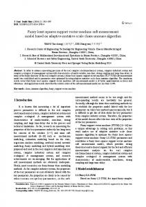
plemented by daptive on–line algorithms. This paper is organized as follows. Sections 2 and 3 describe the structure and functionality of SVM and LS-SVM. The simulation results are presented in Section 4. We will apply the LS-SVM equalizer to time-invariant and time-varying channel problems. Comparisons of the LS-SVM, Bayesian, MLP, and WNN equalizers are shown in this section. Finally, the conclusion is presented in Section 5. 2. Support vector machines In this section, we briefly introduce the standard SVM for binary classification problems. The structure of the standard SVM is shown in Figure 1.

Figure 1. The architecture of the standard SVM model Support vector machines (SVM) have been successfully applied in classification and function estimation problems [12] after their introduction by Vapnik within the context of statistical learning theory and structural risk minimization [14]. Vapnik constructed the standard SVM to separate training data into two classes. The goal of the SVM is to find the hyper-plane that maximizes the minimum distance between any data point. The purpose for training a SVM is to find the classifier f ( x)  x b so that we can use the classifier to classify data. The training l set  xi , yi  , where xi n is the input and i 1 y i  1,1is the output, indicates the class.

Using Least Squares Support Vector Machines for Adaptive Communication Channel Equalization

SVM formulations start from the assumption that the linear separable case is (1)

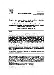
 T ( xi ) b 1, if y i 1 (2) T  ( xi ) b 1, if y i 1  where ( ) denotes a mapping of the input onto a so-called higher dimensional feature space. In this space, a linear decision surface is constructed with special properties that ensure high generalization ability of the network. Its diagram is shown in Fig. 2. By use of a nonlinear kernel function, it is possible to compute a separating hyper-plane with a maximum margin in a feature space.        

(.)

Input space

  

l

can be recovered by using i yi(xi ) , i 1

 T xi b 1, if y i 1 T  xi b 1, if y i 1  For the non-separable case,



rush-Kuhn-Tucker (KKT) conditions. The 



s

t j y t j ( xt j )

(4)

j 1

The quadratic programming problem is solved by considering the dual problem 1 l max  Q()  ij y i y j K ( xi , x j ) 2 i , j 1 0  C , i   l i s.t.  i yi 0   i 1

(5)

with the kernel trick (Mercer Theorem): 

K ( xi , x j ) ( xi ) T ( x j )

(6)









Feature space

Figure 2. Space translation using a nonlinear kernel function We need to find, among all hyper-planes separating the data, an existing maximum 2 margin between the classes. The problem  is transformed into a quadratic programming problem l 1 min T C i 2 i 1

where xi are non-zero values and i are support vectors (SV). The decision boundary is determined only by the SV. Let t j , ( j 1, ..., s ) be the indices of the s support vectors. Then we can rewrite

(3)

s.t yi ( ( xi ) b) 1 i , i 0, i 1,...l T

where C is the trade-off parameter between the error and margin. The quadratic programming problem can be solved by using Lagrangian multipliters i  . The solution satisfies the Ka-

Several types of kernels, such as linear, polynomial, splines, RBF, and MLP, can be used within the SVM. This finally results in the following: l

y ( x) sign(i y i K ( x, xi ) b)

(7)

i 1

3. Least squares support vector machines The standard SVM is solved using quadratic programming methods. However, these methods are often time consuming and are difficult to implement adaptively. Least squares support vector machines (LS-SVM) is capable of solving both classification and regression problems and is receiving more and more attention because it has some properties that are related to the implementation and the computational method. For example, training requires solving a set of linear equations instead of solving the quadratic programming problem involved in the original SVM. The original SVM formulation of Vapnik [9] is Int. J. Appl. Sci. Eng., 2005. 3, 1

53

Cheng-Jian Lin , Shang-Jin Hong, and Chi-Yung Lee

modified by considering equality constraints within a form of ridge regression rather than by considering inequality constraints. The solution follows from solving a set of linear equations instead of a quadratic programming problem. In LS-SVMs, an equality constraint-based formulation is made within the context of ridge regression as follows: l 1 min T C ei2 2 i 1

(8)

s.t y i (T ( xi ) b) 1 ei , i 1,...l One defines the Lagrangian l 1 L(, b, e;)  T C ei2 2 i 1 l

i { yi ( ( xi ) b) 1 ei }

(9)

T

i 1

with Lagrangian multipliers i  . The conditions for optimality are given by l  L  0    i yi( xi )    i 1  l L  0  i yi 0  b i 1  L  0  i Cei i 1, ..l ei   L T  0  yi ( ( xi ) b) 1 ei 0 i 1, ..l i  (10)

By eliminating e, , one obtains the KKT system

0 b   0 YT     (11)     1    1 Y C I     where C is a positive constant, b is the bias, 

y ( y1... yl )T , 1 (1...1), (1...l ) and

ij y i y j( xi ) T ( x j ), 1 i, j l

(12) y i y j K ( xi , x j ) After application of the Mercer condition, the final result is the same as Equation (7). 54

Int. J. Appl. Sci. Eng., 2005. 3, 1

Because LS-SVM does not incorporate the support vector selection method, the resulting network size is usually much larger than the original SVM. To solve this problem, a pruning method can be used to achieve sparseness in LS-SVM [19]. The pruning technique reduces the complexity of the network by eliminating as much hidden neurons as possible. 4. Experimental results In this section, we will demonstrate the validity of the LS-SVM in a communication system. In the experiment, we used a Pentium4 1.5GHz CPU, 512MB of main memory, and the Matlab 6.1 simulation software. High speed communication channels are often impaired by channel Inter-symbol Interference (ISI), Additive White Gaussian Noise (AWGN) and effects of time-varying channels. A discrete time model of a digital communication system is shown in Fig.3. A random sequence xi was passed through a dispersive channel of finite impulse response (FIR) to produce a sequence of outputs yi' . Two kinds of channels, time-invariant and time-varying, were used in our experiment. Additive noise in the system, represented by ei , was then added to each yi' to produce an observation sequence yi . The problem to be considered was how to utilize the information represented by the observed channel outputs yi , yi 1 ,, yi m1 to produce an estimate of the input symbol xi d . A device which performs this function is known as an equalizer. The symbols m and d are known as the order and the delay of the equalizer, respectively. In our experiment, the equalizer order was chosen to be m=2 and delay of the equalizer was chosen to be d=0. Throughout the experiment, the input samples were chosen from {-1,1} with equal probability and were assumed to be independent of one another.

Using Least Squares Support Vector Machines for Adaptive Communication Channel Equalization

The equalizer performance is described by the probability of misclassification with respect to the signal-to-noise ratio (SNR). When an independent identically distributed (i.i.d.) sequence is assumed, the SNR can be defined as 2 SNR 10 log10 s2 (13) e where s2 represents the signal power and e2 is the variance of the Gaussian noise.

following simpler form of the optimal decision function:  y ( n )  y  i ( y ( n ))   exp   i 1 

2

ns  y ( n )  y  i   exp   i 1 

2

n s

fB



  2   2 e

  2   2 e

(15)  1, f B ( y ( n ) 0 x ' ( n ) sgn( f B ( y ( n )))  1, f B ( y ( n ) 0

(16)

Figure 3. Discrete-time model of a data transmission system

where yiand yi refer to the channel states which are the +1 and –1 signal states, which have estimates of the noise-free received signal vector. Therefore, based on the above function, we can decide on the optimal decision boundary. From this point of view, the equalizer can be viewed as a classifier, and the problem can be considered as a classification problem.

4.1. Bayesian equalizer

4.2. The time-invariant channel problem

The Bayesian decision theory provides the optimal solution to the general decision problem. Therefore, the optimal symbol-by-symbol equalizer can be formed from the Bayesian probability theory and is termed a Bayesian or a maximum posteriori probability (MAP) equalizer. This minimum error probability decision can be rewritten as  y ( n ) y  2  i  exp  2  2e  i 1   2  m ns  y ( n ) y   i   p j ( 2e2 ) 2 exp  2   2  e i 1   n s

f B ( y ( n ))  p i ( 2e2 )

m 2

(14) where e denotes the standard deviation (std) of the Gaussian additive noise e(k). For equiprobable symbols, the coefficients p j (2e2 )

m 2

in f B ( y (n)) become redundant and can be removed. This gives rise to the

Let the channel transfer function be y ' ( n ) ( n ) 0 . 1 ( n ) 3

( n ) a1 x ( n ) a 2 x ( n 1)

(17)

where a1=0.5 and a2=1. Then the output channel signal is

y ' ( n ) ( 0 . 5 x ( n ) x ( n 1)) 0 . 1 ( 0 . 5 x ( n ) x ( n 1)) 3

(18)

All the combinations of x(n) and the desired channel states are listed in Table 1. To see the actual bit error rate (BER), a realization of 106 points of sequence y(n) were used to test the BER of the LS-SVM equalizer. The resulting BER curve of the LS-SVM equalizer under different SNRs is shown in Fig. 4. When the level of the noise was 10db, 1000 samples of y(n) were used for training, as shown in Figure 5. We tested the performance of the Bayesian, LS-SVM, multilayer perceptron (MLP), and Int. J. Appl. Sci. Eng., 2005. 3, 1

55

Cheng-Jian Lin , Shang-Jin Hong, and Chi-Yung Lee

wavelet neural network (WNN) equalizers. The Bayesian equalizer was the most optimal method for communication channel equaliza tion. Computer simulation results showed that the bit error rate of the LS-SVM equalizer was close to the optimal equalizer and better than the MLP and WNN equalizers.

Table 1. Input and desired channel states for m=2 and d=0 x(n-1) x(n-2)

y ’ ( n )y ‘ ( n-1)

NO

x(n)

1

1

1

1

1.8375 1.8375

2

1

1

-1

1.8375 -0.5125

3

1

-1

1

-0.5125 0.5125

4

1

-1

-1

-0.5125 -1.8375

5

-1

1

1

0.5125 1.8375

6

-1

1

-1

0.5125 -0.5125

7

-1

-1

1

-1.8375 0.5125

8

-1

-1

-1

-1.8375 -1.8375

4.3. The time-varying channel problem

Figure 4. Comparison of bit-error-rate curves for the Bayesian, LS-SVM, MLP, and WNN equalizers in a time-invariant channel

Figure 5. Time-invariant channel, data clusters from LS-SVM, SNR=10db,1000 samples of y(n), and decision boundary

56

Int. J. Appl. Sci. Eng., 2005. 3, 1

Let the nonlinear time-invariant channel transfer function be as given by Eq. (16) where a1 =0.5 and a2 =1. Since we assume the channel is time-varying, a1 and a2 are two time-varying coefficients. These time-varying coefficients were generated by passing white Gaussian noise through a Butterworth low pass filter (LPF). The example was centered at a1 =0.5 and a2 =1, and the input for the Butterworth filter was a white Gaussian sequence with standard deviation (std) . Applying the function provided by Matlab, we can generate a second-order low pass digital Butterworth filter with cutoff frequency =0.1. Adjusting the time-varying coefficients, we plotted the coefficients and the corresponding channel states, as shown in Figs. 6(a) and 6(b), respectively. The resulting BER curves of the Bayesian, LS-SVM, MLP, and WNN equalizers under different SNRs are shown in Figure 7. Our method obtained a better BER curve. According to the experimental results, we see that the classification rate of the LS-SVM equalizer is better than that of some of the

Using Least Squares Support Vector Machines for Adaptive Communication Channel Equalization

(a)

(b)

(c)

(d)

Figure 6. (a) An example of a time-invariant channel; (b) channel states (noise free) of the time-invariant channel; (c) an example of a time-varying channel with =0.1; and (d) channel states (noise free) of the time-varying channel other existing models for channel equalization problems. Table 2 shows the hardware computation time for training and testing when the channel’ s SNR was 10db. The training time for the Bayesian equalizer was zero because it did not need to be trained. The WNN with the simultaneous Perturbation method [20] was adopted to solve the channel equalization problem and converged after 2000 iterations. The MLP also used the traditional back-propagation algorithm, and its convergence happened after 1000 iterations. We can see that the training and testing times for the LS-SVM equalizer are faster Figure 7: Comparisons of bit-error-rate curves for than those for the WNN and MLP equalizers. the Bayesian, LS-SVM, MLP and WNN For this reason, the LS-SVM equalizer is equalizers in a time-varying channel more suitable for adaptive communication with = 0.1 channel equalization. Int. J. Appl. Sci. Eng., 2005. 3, 1

57

Cheng-Jian Lin , Shang-Jin Hong, and Chi-Yung Lee

Table 2. The hardware computation times for various equalizers Model

Bayesian (sec)

LS-SVM (sec)

WNN (sec)

MLP (sec)

Training time (Time varying channel)

-

15.36

5045

2011

Testing time (Time varying channel)

511.24

398.45

660.48

543.8

Training time (Time invariant channel)

-

14.97

4583

1997

Testing time (Time invariant channel)

505.99

399.31

602.42

560

Process

5. Conclusion In this paper, we adopted least squares support vector machines (LS-SVM) for adaptive communication channel equalization. The LS-SVM equalizer has the advantage of being able to be implemented with relatively low complexity and good performance. We applied the LS-SVM equalizer to the time-invariant and time-varying channel problems. Simulation results showed that the bit error rate of the LS-SVM equalizer is close to the Bayesian equalizer and better than the MLP and WNN equalizers. Reference [ 1] Al-Mashouq, K. A. and I. S. Reed. 1994. The use of neural nets to combine equalization with decoding for severe intersymbol interference channels. IEEE Transactions on Neural Networks, 5, 6: 982-988.

58

Int. J. Appl. Sci. Eng., 2005. 3, 1

[ 2] Chen, S., B. Mulgrew, and P. M. Grant. 1993. A clustering technique for digital communications channel equalization using radial basis function networks. IEEE Transactions on Neural Networks, 4, 4: 570-579. [ 3] Liang, Q. and J. M. Mendel. 2000. Equalization of nonlinear time-varying channels using type-2 fuzzy adaptive filters. IEEE Transactions on Fuzzy Systems, 8, 5: 551 - 563. [ 4] Jagdish, C. Patra and Ranendra N. Pal 1995. A functional link artificial neural network for adaptive channel equalization. Elsevier Science B. V. Signal Processing, 43: 181-195. [ 5] Kechriotis, G. and E. S. Manolakos. 1994. Using recurrent neural networks for adaptive communication channel equalization. IEEE Transactions on Neural Networks, 5, 2: 267-278. [ 6] Gibson, G. J. and C. G. N. Cowan. 1990. On the decision regions of multilayer

Using Least Squares Support Vector Machines for Adaptive Communication Channel Equalization

[ 7]

[ 8]

[ 9]

[10]

[11]

[12]

[13]

[14]

perceptrons. Proceedings of the IEEE, 78: 1590-1594. Cristea, P., R. Tuduce, and A. Cristea. 2000. Time series prediction with wavelet neural networks. Proceedings of IEEE Neural Network Applications in Electrical Engineering. Zhang, J., G. G. Walter., Y. Miao, and W. N. W. Lee. 1995. Wavelet neural networks for function learning. IEEE Trans. on Signal Processing, 43: 1485-1497. Cortes, C. and V. Vapnik. 1995. Support vector networks. Machine Learning, 20, 3: 273-297. Muller, K.-R., S. Mika., G. Ratsch., K. Tsuda, and B. Scholkopf. 2001. An introduction to kernel-Based learning algorithms. IEEE Transactions on Neural Networks. 12, 2: 181-202. Suykens, J. A. K. and J. Vandewalle, 1999. Least squares support vector machine classifiers. Neural Processing Letters. 9, 3: 293-300. Cristianini, N. and J. Shawe-Taylor. 2000. “ An introduction to support vector machines and other kernel based learning methods”. Cambrige University Press. Poggio, T. and F. Girosi. 1990. Networks for approximation and learning. Proceeding of the IEEE, 78, 9: 1481-1497. Vapnik, V. 1995. “TheNat ur eofSt a t i stical Learning Theory.”Springer-Verlag New York, Inc.

[15] El-Naqa, I., Y. Yang., M. N. Wernick., N. P. Galatsanos, and R. M. Nishikawa. 2002. A support vector machine approach for detection of microcalcifications. IEEE Transactions on Medical Imaging. 21, 12: 1552-1563. [16] Valentini, G., M. Muselli, and F. Ruffino. 2003. Bagged ensembles of support vector machines for gene expression data analysis. Proceedings of the International Joint Conference on Neural Networks. 3: 20-24. [17] Kim, K. I., K. Jung., S. H. Park, and H. J. Kim. 2002. Support vector machines for texture classification. IEEE Transactions on Pattern Analysis and Machine Intelligence. 24, 11:1542-1550. [18] Malinowski, M., M. Jasin´ski, and M. P. Kazmierkowski. 2004. Simple direct power control of three-phase PWM rectifier using space-vector modulation (DPC-SVM). IEEE Transactions on Industrial Electronics. 51, 2:447-454. [19] Suykens, J. A. K., L. Lukas, and J. Vandewalle. 2000. Sparse least squares support vector machine classifier. ESANN’ 2000 European Symposium on Artificial Neural Networks: 37-42. [20] Maeda, Y. and R. J. P. De Figueiredo. 1997. Learning Rules for Neuro-Controller via Simultaneous Perturbation. IEEE Transaction on Neural Networks. 8, 5:1119-1130.

Int. J. Appl. Sci. Eng., 2005. 3, 1

59