doi 10.1098/rspb.2000.1236
Using probability of persistence to identify important areas for biodiversity conservation Paul H. Williams* and Miguel B. Arau¨jo Biogeography and Conservation Laboratory,The Natural History Museum, Cromwell Road, London SW7 5BD, UK Most attempts to identify important areas for biodiversity have sought to represent valued features from what is known of their current distribution, and have treated all included records as equivalent. We develop the idea that a more direct way of planning for conservation success is to consider the probability of persistence for the valued features. Probabilities also provide a consistent basis for integrating the many pattern and process factors a¡ecting conservation success. To apply the approach, we describe a method for seeking networks of conservation areas that maximize probabilities of persistence across species. With data for European trees, this method requires less than half as many areas as an earlier method to represent all species with a probability of at least 0.95 (where possible). Alternatively, for trials choosing any number of areas between one and 50, the method increases the mean probability among species by more than 10%. This improvement bene¢ts the least-widespread species the most and results in greater connectivity among selected areas. The proposed method can accommodate local di¡erences in viability, vulnerability, threats, costs, or other social and political constraints, and is applicable in principle to any surrogate measure for biodiversity value. Keywords: biodiversity; probability of persistence; e¤ciency; area-selection methods 1. INTRODUCTION
Many statutor y obligations now require networks of protected areas to be established for the conservation of biodiversity. But because competing interests limit the opportunities for conservation, great emphasis has been placed on the e¤ciency with which networks represent numbers of species (e.g. Pressey & Nicholls 1989; Rebelo & Siegfried 1992; Pressey et al. 1993; Pressey & Tully 1994; Rodrigues et al. 1999; Williams et al. 2000). Nonetheless, all of these authors appreciated that ultimately it is not how many species have been recorded within a set of areas that is important for conservation, but how many will persist there for the future. This idea of persistence has been discussed before as an ideal (e.g. Margules et al. 1994; Faith & Walker 1996a; Williams 1998; Cowling et al. 1999; Virolainen et al. 1999), although so far no areaselection studies have taken a consistently probabilistic approach to persistence. We address directly the overarching idea of longer-term conservation success by describing a quantitative method for selecting networks of conservation areas using species’ probabilities of persistence. This paper is concerned not with how to estimate probabilities of persistence, but with how to use this information. This is not to say that these estimates are easy to obtain. For most species, the best information that can be expected is presence data (Van Jaarsveld et al. 1998). In this case, one starting point is species’ local probabilities of occurrence, which can be estimated by modelling habitat suitability and species’ dispersal (Arau¨jo & Williams 2000). Converting occurrence probabilities into estimates of persistence probabilities depends upon including the time dimension (for probability of occurrence at a particular time horizon in the future) and upon considering the added risk from the combination of local *
Author for correspondence (
[email protected]).
Proc. R. Soc. Lond. B (2000) 267, 1959^1966 Received 26 January 2000 Accepted 12 July 2000
threats and each species’ vulnerabilities. Some of these aspects can also be estimated or modelled (e.g. Burgman et al. 1993; Menges 2000). Expressing the consequences of these di¡erent pattern and process factors in terms of their e¡ect on probabilities of persistence would allow them to be integrated in a consistent way (Williams & Arau¨jo 2000). There are undoubtedly many di¤culties with this approach (Ludwig 1999), although as long as it allows the areas with the worst persistence prognoses to be avoided, then there is still a useful role for the approximate estimates that can be obtained. When information related to the species’ di¡ering local probabilities of persistence is available, area-selection methods have almost always dealt with it by resorting to crude thresholds to exclude areas where species have a poor prognosis (e.g. Bedward et al. 1992; Kershaw et al. 1994; Polasky et al. 2000). In e¡ect, this converts probabilities to presence^absence data, losing much of the information. In contrast, Margules & Nicholls (1987) proposed an area-selection method for vegetation classes that uses directly probabilities of occurrence. Their method could be applied to probabilities of persistence but, as we show, it is even less e¤cient in terms of probability than using the original presence data from which the probabilities were modelled. This is important, because ine¤ciency means lost opportunities for protecting more of valued biodiversity. In this paper, we demonstrate a new method for handling probabilities, using simple rules that seek to maximize the expected success for conservation. 2. DATA AND METHODS Our analysis starts with records of species’ presence from a distribution atlas. We use 54 427 records for the current distribution of 148 species and subspecies of European trees, which include most of the important timber species. These are a subset of the Atlas Florae Europaeae (AFE) data, mapped on the
1959
© 2000 The Royal Society
1960
P. H. Williams and M. B. Arau¨jo
Conservation by probability ofpersistence
50 £ 50 km cells of the universal transverse mercator (UTM) grid ( Jalas & Suominen 1972^1994). The area covered spans 2203 grid cells in Western Europe, excluding most of the former Soviet Union, but including the Baltic States, because sampling e¡ort within this region has been relatively intensive and uniform (Lahti & Lampinen 1999). From these data, Arau¨jo & Williams (2000) used niche-based regression models to estimate species’ local probabilities of occurrence. Information on threat and vulnerability is in preparation. For the present, if we assume that appropriate conservation management could largely ameliorate these added risks within the selected areas, then we might expect probabilities of persistence to be correlated with probabilities of occurrence. This would allow these probabilities to be used as ¢rst-approximation surrogates for the purposes of illustrating the principles of the area-selection method at the next step. Probability estimates are included in the area-selection data only for those areas where presence records occur in the original atlas data, and any estimates of less than 0.05 are set to zero, as an arbitrary threshold for `quasiextinction’ (Ginzburg et al. 1982). At the scale of 50 £ 50 km cells, probabilities for the di¡erent areas are assumed initially to be e¡ectively independent of one another when selecting areas (but see ½ 4). Because these data are used purely as an example to compare the consequences of using species’ local probability estimates in area selection, the results should not be interpreted as an attempt to propose a new protected area network for Europe. We consider both of the common forms of area-selection problems (Camm et al. 1996). First is the minimum-set problem, such as `What is the minimum set of areas required to represent all species with a probability of at least 0.95?’ Second is the maximum-coverage problem, such as `Which set of 50 areas can represent all species with the maximum probability across all species ?’ To simplify comparisons, we treat the near-equal-area grid cells as being of equal `cost’, so the optimization is applied to the number of areas. However, when cost data for individual areas are available (using `cost’ in the broadest sense, not just for monetary costs), area-selection methods can be used to optimize against cost rather than area constraints (see table 1, step 2d). This helps selection methods to deal appropriately with areas of any shape and size, not just with equal-area cells within a regular grid. We compare three quantitative area-selection methods for both minimum-set and maximum-coverage problems. The ¢rst method, applied to the original presence data (the `presence method’) treats all records for a species as equivalent, and uses a popular technique based on selecting those areas richest in the rarest species at each step (Margules et al. 1988). Checks to exclude redundant areas have been added to improve e¤ciency. Re-ordering of selected areas by complementary richness may then be used to give approximate solutions to maximum-coverage problems (Williams 1998), as demonstrated in Csuti et al. (1997, algorithm 8). For the European trees, the ¢rst 50 areas from a re-ordered near-minimum set provide a near-maximum coverage solution. Once these areas have been selected using the presence data, the probability data for the selected areas can be used to calculate probabilities (p i) for each species (i) combined among these areas. Local probabilities of persistence (p ij) for species i in area j are combined among n areas using the product of probabilities of local non-persistence (extirpation): p i ˆ 1 ¡ ¦j ˆ 1
: : : n (1
¡ p ij ).
Proc. R. Soc. Lond. B (2000)
(1)
The second method was proposed by Margules & Nicholls (1987) to represent mallee vegetation using probabilities of occurrence (the `mallee method’). Initially, it selects those areas with the highest individual probabilities for each of the species to be represented. The second set of area choices depends on which areas would give the greatest incremental increases in probability for each species. Species are ignored once they have reached their representation goal, otherwise selection continues for the remaining species. If ties occur at any step, then the ¢rst area encountered is selected. For the maximum-coverage problem, the ¢rst 50 areas from the original order of selection are used. The third method is described in detail in table 1 (the `new method’ or goal^gap method), and a worked example is given in Appendix A. In outline, the method begins by selecting all of the `irreplaceable’ areas (table 1, step 1). These include all of the areas for any species with total combined probabilities among areas (from equation (1)) of less than the representation goal. The method then chooses one area at each iteration (table 1, step 2), by examining by how much choosing each area would contribute incrementally to reaching the representation goal for each species, and choosing the area that contributes the most across all species. If ties occur for any choice, then the area with the highest sum of probabilities across all species is selected. For addressing maximum-coverage problems, there are two options. First, the probability goal can be adjusted until an approximation to the required number of areas is obtained (for 50 areas for European trees, this goal would be p g(i) 5 0.79, resulting in a mean combined probability among species of 0.95, lower quartile 0.96). Alternatively, a set of areas selected for a higher goal (e.g. p g(i) 5 0.95) can be re-ordered using the same selection procedure that was used to select them, but without choosing irreplaceable areas ¢rst. This brings the areas with the greatest incremental contribution to the goal to the top of the list, and then the ¢rst 50 of these areas are used. Here we use the second approach (table 1, steps 3^4) which, while it may give lower probabilities for a few of the rarer species, is quicker and gives a higher mean probability among all species (50 areas from within a minimum set of 79 areas for a goal of p g(i) 5 0.95 results in a mean combined probability among species of 0.97, lower quartile 0.99). To assess the success of the three area-selection methods, areas are chosen by random draws without replacement 1000 times for each number of areas required, and the mean of the combined probabilities for the tree species represented in these area sets is calculated. All area-selection methods were automated using the WORLDMAP software (Williams 1999). 3. RESULTS
The species representation achieved when seeking minimum-area sets by the three area-selection methods is shown in table 2. In seeking a representation target explicitly in terms of probability (p g(i)5 0.95), the two probability methods succeed in achieving a higher probability across all species than the presence method, but they also require more than three times as many areas. The new method requires less than half as many areas to reach the target as the mallee method. Any method that selects more areas would be expected to result in higher probabilities for this reason alone. Maximum-coverage solutions can provide comparisons on a per-unit-area basis, thereby controlling for this
Conservation by probability ofpersistence Table 1. A `goal^gap ’ method to select areas using probability data (see Appendix A for an example) (Probabilities are combined as shown in equation (1). Rules 1^ 2 are used to select a near-minimum cost-set of areas to represent all species with a combined probability of at least p g(i), using probability data ( p i j) for species i in area j (see Appendix A). Rules 3^4 are added to select a near-maximum coverage set for a given number of areas or budget.) step 1 a b c
2 a
b
c d e f g
3
4 5
rule For gap analysis, begin with the set of adequately protected areas, ¢nd the corresponding combined species probabilities, then select all irreplaceable areas: select all areas with species that have a total combined probability (p i ) less than the representation goal (p g(i)); calculate the combined representation probability of all species among selected areas (p i ); all data (p i j ) for any species that have reached their realizable representation goal, and all data for any selected areas, are set to zero (to ensure complementarity). The following rules are then applied repeatedly until all species are represented: calculate the potential contribution of each record in the matrix to increasing the combined representation probability above the current combined representation probability; calculate the part of the potential contribution of each record in the matrix to ¢lling the gap between the current combined representation probability and the representation goal; sum these goal^gap contributions for all species yet to be fully represented for each area; select the area with the highest summed goal^gap contribution or, if cost data are available, choose the area with the highest (summed contribution)/cost ratio; if there are ties (areas with equal scores), select the area with the largest sum of probabilities across all species without complementarity (total p j); calculate the combined representation probability of species among selected areas (p i ); all data (p i j) for the species that have reached their representation goal, and all data for any selected areas, are set to zero (to ensure complementarity). (Rep eat step s 2a^g until all sp ecies meet the representation goal.) For maximum-coverage problems, the set of selected areas from steps 1^2 may be re-ordered by re-applying the rules in step 2 a^g to produce a series of approximate solutions for maximizing mean probability across all species. For maximum-coverage problems, choose the required number (or cumulative cost) of areas starting from the beginning of the re-ordered area list. For prioritizing selected areas for urgency of management action, they may be re-ordered by their degrees of risk (threat and vulnerability).
factor. The species representation achieved when seeking maximum-coverag e sets of from one to 50 areas is shown in ¢gure 1. All three methods represent species with a signi¢cantly higher mean probability (among all 148 species and subspecies) than would be expected from selecting areas at random (except for the ¢rst area choice by the mallee method). Within this range of numbers of areas selected, the relative performance of the three Proc. R. Soc. Lond. B (2000)
P. H. Williams and M. B. Arau¨jo 1961
Table 2. Species-representation results for near-minimum-area sets area-selection method presence method (based on Margules et al. 1988) mallee method (Margules & Nicholls 1987) new method (table 1) (all areas)
number of areas selected
mean probability among all species within areas selected
25
0.78
182
0.97
79 2203
0.97 0.97
methods in terms of mean probability is consistently : new method 4 presence method (mean increase 10.1%) 5 mallee method (mean increase 6.3%). By comparing the spatial consequences of selecting a maximum-coverag e set of 50 areas, we ¢nd that all three methods select areas that are widely scattered among all regions of Europe. However, the areas selected by the two probability methods from these data are more clustered into local groups (mean number among the eight nearest neighbours of selected areas that are themselves selected areas: presence method, 6.5%; mallee method, 8.25%; new method, 8.5%). Switching from using presence data to using the new probability method increases the combined probability between the 50-area sets for most of the species with lower probabilities. This is shown in ¢gure 2a by most of the points being displaced above the diagonal (solid line). Indeed, an additional 11% of species reach the representation goal with the new method (133 species above upper dashed line in ¢gure 2a for p g(i)5 0.95) compared with the presence method (116 species beyond the dashed line to the right of ¢gure 2a for p g(i) 5 0.95). Ignoring the small changes for species that exceed the goal by both methods (upper right dashed quadrant of ¢gure 2a), then 25 species show an increase in probability (mean increase 0.33), whereas only one species shows a small decrease in probability ( 7 0.06). Figure 2b shows that the 25 species with increased probabilities are among the species with the most restricted distribution ranges within Europe. 4. DISCUSSION
We show that the advantage of using probability data rather than presence data for area selection is a greater expectation of conservation success. The expected probabilities of persistence are higher among the species. For these data, the selected areas are also more clumped locally, reducing the `Noah’s Ark’ e¡ect of selecting small isolated patches (Pimm & Lawton 1998). A particular strength of the approach is that it gives the greatest bene¢ts for the species with lowest persistence probabilities (¢gure 2a) and most restricted distributions (¢gure 2b). The new selection method provides an approximation to truly optimal area sets. Area-selection problems of this form are `not polynomial complete’, in that the exact size of the problem cannot be calculated simply from the amount of data. For representing I species at least once from presence^absence data, the solution lies in a combination of between one and I areas, whereas for achieving
1962
P. H. Williams and M. B. Arau¨jo
Conservation by probability ofpersistence
1.0
mean probability among all species
0.8
0.6
0.4 new method presence method mallee method random 95% upper tail
0.2
0.0
0
5
10
15
20 25 30 number of areas selected
35
40
45
50
Figure 1. Mean of the combined probabilities among all 148 species and subspecies of trees when between one and 50 areas are selected using three methods: a representation method for use with presence data (based on Margules et al. 1988); the mallee probability method (Margules & Nicholls 1987); and a new probability method (table 1). Scores below the dashed line are within the range expected when choosing areas at random. Areas are 50 £ 50 km cells of the Atlas Florae Europ aeae grid.
a probability goal, the solution lies in a combination of between one and all (J) areas. Most area-selection problems are too large to allow an exhaustive search for the solution (e.g. Polasky et al. 2000). Branch and bound methods can reduce the size of the problem, but these are more complex to implement and slower to run (Cocks & Baird 1989). The degree of sub-optimality in our heuristic approximation has not been assessed here, although by analogy with the results of using presence data (Pressey et al. 1996, 1997; Csuti et al. 1997), it is expected to be small relative to uncertainties in the data and the constraints of turning results into conservation action. At the least, the new method o¡ers a substantial improvement in e¤ciency over widely accepted earlier methods (table 2, ¢gure 1). This comes in part from choosing areas that contribute most across all species to ¢lling the gaps between current representation and their representation goals. The mallee method is also less e¤cient because it chooses many areas at each iteration, without taking into account complementarity among their biota. The principal challenge for the probability approach is whether useful (rather than necessarily very precise) estimates of the probability of local persistence for the species can be obtained (Ludwig 1999). We often lack knowledge as to precisely which factors govern the probabilities for the species at any particular time and place, as well as lacking good data for these factors. Furthermore, not all aspects of the external threat or the internal dynamics of populations will be inherently predictable. However, this should not prevent e¡orts to try to reach useful predictions, particularly when enough is known at least to Proc. R. Soc. Lond. B (2000)
exclude the worst options. Consequently, it should be possible to reach estimates of probability of persistence that improve upon treating all species’ presence records as equivalent (Arau¨jo & Williams 2000). This should reduce the need for relying on simple `rules of thumb’, which may not always have the same value (e.g. the single large or several small (SLOSS) debate). For example, our suitability models imply that species are more likely to persist (if threats were uniformly distributed) near the cores of their environmental-niche space (which may correspond broadly to their geographical range centres). In apparent contrast, Channel & Lomolino (2000) have shown that populations in the cores of species’ geographical ranges were often extirpated historically before populations in the periphery, which they suggest was caused by patterns of threat. These two patterns do not contradict one another, but relate to di¡erent components of the conservation problem (suitability and threat), which need to be integrated if we are to achieve realistic estimates of persistence probabilities before areas are selected. Arau¨jo & Williams (2000) describe a framework and some simple models. A major concern for conservation is the e¡ect of climate change. This could be incorporated by modelling future habitat suitability in the estimation of probabilities of persistence. With changing suitability, areas of high present and future suitability will need to be in close proximity relative to species’ dispersal abilities if they are to persist (Huntley 1998). There is considerable potential for expanding these models to include interdependencies of local probabilities, both among species within areas, and
Conservation by probability ofpersistence
species probability from new method ( pN)
1.0
(a)
0.8
0.6
0.4
0.2
0.0 0.0 change in probability between new and presence methods (pN - pP)
P. H. Williams and M. B. Arau¨jo 1963
0.8
0.2 0.4 0.6 0.8 species probability from presence method ( pP)
1.0
(b)
0.6
0.4
0.2
0.0
- 0.2
0
200
400
600
800 1000 1200 European range size
1400
1600
1800
Figure 2. Change in probabilities for each species between the presence method and the new probability method. (a) Combined probabilities ( p i) for all 148 species and subspecies of trees when a set of 50 areas is selected for maximum coverage using a new method (table 1) for use with estimated probabilities of persistence ( p N), plotted against combined probabilities from a set of 50 areas selected for maximum coverage using a method for use with presence data (based on Margules et al. 1988) ( p P). The dashed lines show the probability goal ( p g(i) 5 0.95). (b) Di¡erence between the new method and the presence method ( p N 7p P) in the combined probabilities for the 148 species and subspecies of trees when a set of 50 areas is selected for maximum coverage, plotted against range size within Western Europe. Species that reach the goal by both methods are not included and range size is measured as the number of areas with records. For both plots, the diagonal line follows equal probabilities from the two methods. Areas are 50 km £ 50 km cells of the Atlas Florae Europaeae grid.
for each species among areas (Menges 2000). This could be used for a more inclusive treatment of processes, including interspecies interactions, the e¡ects of dispersal among areas, and dependencies of species on more distant feeding, migration, and overwintering areas. Some of these dependencies may demand that probabilities be re-estimated dynamically from the models at each step of area selection. Many non-biological factors may act as constraints on achieving conservation goals (e.g. Goldsmith 1991; Pressey et al. 1993). Many of these can already be accommodated by quantitative methods (see table 1). Examples Proc. R. Soc. Lond. B (2000)
include starting with an existing set of protected areas (i.e. performing a `gap analysis’ for complementing a subset of species that has some existing protection; Scott et al. 1993), and using information on the relative costs of selecting areas (Faith & Walker 1996b). These `costs’ may include not only the ¢nancial costs of acquiring and managing areas, but also the opportunity costs of the income foregone when excluding other incompatible land uses, such as certain forms of logging, agriculture, or other commercial development. Some of the other social and political constraints (McNeely 1997) might be
1964
P. H. Williams and M. B. Arau¨jo
Conservation by probability of persistence
treated in a similar way, for example, by selecting areas to minimize the number of people a¡ected. Subsequently, selected areas can be prioritized for urgency of management action, by re-ordering areas by their degrees of risk, taking into account threats and species’ corresponding vulnerabilities. Prendergast et al. (1999) have argued that the greatest problems for applying quantitative methods for practical conservation stem from a lack of communication and funding. Many land managers are either unaware of the methods, or perhaps more often, unaware of how they can be used to get the most from their local expert knowledge. While more surveys are needed, there is also a need for quantitative methods to be passed to land managers in a form that can help them explore and communicate the
wealth of existing knowledge. This will help people to appreciate that modelling is just a tool for getting the most out of this knowledge in an accountable way, while decision-support software such as WORLDMAP merely makes area-selection procedures easily accessible and applicable to large numbers of species. Combining these resources would go some way to improving the chances of conserving biodiversity, even when using very simple surrogates for the major factors a¡ecting species’persistence. The AFE presence data were provided by T. Lahti and R. Lampinen of the Botanical Museum, Finnish Museum of Natural History, Helsinki. We thank C. Humphries, R. VaneWright and referees for comments. M.B.A. is funded by a Portuguese FCT/PRAXIS XXI studentship, no. BD/9761/96.
APPENDIX A
Example of the application of the goal^ gap method from table 1 to some simple example data for the probabilities of persistence (p ij ) of eight species (i) among six areas ( j). The goal is to represent all species with a probability p g(i)5 0.5 in a near-minimum number of areas. species (i) area ( j) 1 2 3 4 5 6
a 0 0.2 0 0.2 0 0
b 0.2 0.4 0 0.6 0 0
c 0.4 0.4 0 0.2 0 0
d 0.6 0.2 0 0 0 0
e 0.4 0 0.2 0 0 0
f 0.2 0 0.4 0 0.4 0
g 0 0 0.4 0 0.6 0
h 0 0 0.2 0 0.4 0.1
p ij
(a) Step 1. Select irreplaceable areas
Step 1a. Calculate combined probability of persistence from the products of the probabilities of local extirpation (nonpersistence): species (i) combined p i
a 0.36
b 0.81
c 0.71
d 0.68
e 0.52
f 0.71
g 0.76
h 0.57
1 ˆ ¦j ˆ 1...6(17 p i j).
The maximum level of representation achievable for species a is only 0.36, so all areas with species a (areas 2 and 4) will be irreplaceable with respect to this reduced (but realizable) representation goal (p g(a) ˆ 0.36). Step 1b. After selecting areas 2 and 4, the combined representation of each species will be combined p i
0.36
0.76
0.52
0.2
ö
ö
ö
ö
17 ¦ j ˆ 2,4(17 p i j).
Consequently, species a, b and c are considered to have achieved their representation goals (p g(b,c) 5 0.5). Step 1c. All selected areas and all species that have reached their representation goal can now be ignored: area ( j) 1 3 5 6
ö ö ö ö
ö ö ö ö
ö ö ö ö
0.6 ö ö ö
0.4 0.2 ö ö
0.2 0.4 0.4 ö
ö 0.4 0.6 ö
ö 0.2 0.4 0.1
(b) Step 2, iteration 1. Select area with maximum goal^ gap increment
p i j.
Step 2a. The increased representation with the selection of each candidate area can be calculated for each record in the matrix from the product of their probabilities of local extirpation. Species d already has some representation (0.2) from step 1 of the method, so its combined probability of extirpation if area 1 were added would become 0.8 £ 0.4 ˆ 0.32: species ( i) area ( j) 1 3 5 6
a 1.0 1.0 1.0 1.0
b 1.0 1.0 1.0 1.0
c 1.0 1.0 1.0 1.0
d 0.32 1.0 1.0 1.0
e 0.6 0.8 1.0 1.0
f 0.8 0.6 0.6 1.0
g 1.0 0.6 0.4 1.0
h 1.0 0.8 0.6 0.9.
ö 0.4 0.6 ö
ö 0.2 0.4 0.1.
These ¢gures are converted back to increased probabilities of persistence: area ( j) 1 3 5 6 Proc. R. Soc. Lond. B (2000)
ö ö ö ö
ö ö ö ö
ö ö ö ö
0.68 ö ö ö
0.4 0.2 ö ö
0.2 0.4 0.4 ö
Conservation by probability ofpersistence
P. H. Williams and M. B. Arau¨jo 1965
Step 2b. The potential contribution of each record in the matrix to ¢lling the gap between the current representation and the representation goal within the range of this increased representation can be calculated (below). Step 2c. The potential contribution is summed for each area, as shown on the right: area ( j) 1 3 5 6
ö ö ö ö
ö ö ö ö
ö ö ö ö
0.3 ö ö ö
0.4 0.2 ö ö
0.2 0.4 0.4 ö
ö 0.4 0.5 ö
ˆ 0.9 ˆ 1.2 ˆ 1.3 ˆ 0.1.
ö 0.2 0.4 0.1
Step 2d. Area 5 would make the largest incremental contribution (1.3) to reaching the overall representation goal at this step. If data for area cost (cj) were available, then the incremental score for each area would be (p j/cj). Step 2e. The tie-breaking step is not required in this case because there are no tied scores. Step 2f. After selecting areas 2, 4 and 5, the combined representation of each species will be combined p i
0.36
0.76
0.52
0.2
ö
0.4
0.6
0.4
1 7 ¦ j ˆ 2,4,5 (17 p i j).
Consequently, species a, b, c and g are considered to have achieved their representation goals. Step 2g. All selected areas and all species that have reached their representation goal can now be ignored: area ( j) 1 3 6
ö ö ö
ö ö ö
ö ö ö
0.6 ö ö
0.4 0.2 ö
0.2 0.4 ö
ö ö ö
ö 0.2 0.1.
(c) Step 2, iteration 2. Select area with next maximum goal^ gap increment
The potential contribution of each record in the matrix to ¢lling the gap between the current representation and the representation goal within the range of this increased representation is again calculated and summed for each area: species (i) area ( j) 1 3 6
a ö ö ö
b ö ö ö
c ö ö ö
d 0.3 ö ö
e 0.4 0.2 ö
f 0.1 0.1 ö
g ö ö ö
h ö 0.1 0.1
incremental p j ˆ 0.8 ˆ 0.4 ˆ 0.1.
Area 1 would make the largest incremental contribution (0.8) to reaching the overall representation goal at this step. After selecting areas 2, 4, 5 and 1, the combined representation of each species will be combined p i
0.36
0.81
0.71
0.68
0.6
0.52
0.6
0.4
1 7 ¦ j ˆ 1,2,4,5(17 p i j).
Consequently, species a^ g are considered to have achieved their representation goals. All selected areas and all species that have reached their representation goal can now be ignored: area ( j) 3 6
ö ö
ö ö
ö ö
ö ö
ö ö
ö ö
ö ö
0.2 0.1.
(d) Step 2, iteration 3. Select area with next maximum goal^ gap increment
The potential contribution of each record in the matrix to ¢lling the gap between the current representation and the representation goal within the range of this increased representation is again calculated and summed for each area: species (i) area ( j) 3 6
a ö ö
b ö ö
c ö ö
d ö ö
e ö ö
f ö ö
g ö ö
h 0.1 0.1
incr p j ˆ 0.1 ˆ 0.1
(total p j ) (1.2) (0.1).
There is a tie between areas 3 and 6 for making the largest incremental contribution (0.1) to reaching the overall representation goal at this step. One way of breaking ties is to choose the area with the largest sum of probabilities across all species without complementarity (total p j). After selecting areas 2, 4, 5, 1 and 3, the combined representation of each species will be: combined p i
0.36
0.81
0.71
0.68
0.52
0.71
0.76
0.52
1 7 ¦j ˆ 1,2,3,4,5(17 p i j).
Consequently, all species (a^ h) are considered to have achieved their realizable representation goals. REFERENCES Arau¨jo, M. B. & Williams, P. H. 2000 Selecting areas for species persistence using occurrence data. Biol. Conserv. 96, 331^395. Bedward, M., Pressey, R. L. & Keith, D. A. 1992 A new approach for selecting fully representative reserve networks: addressing e¤ciency, reserve design and land suitability with an iterative analysis. Biol. Conserv. 62, 115^125. Burgman, M. A., Ferson, S. & Akc°akaya, H. R. 1993 Risk assessment in conservation biology. London: Chapman & Hall. Proc. R. Soc. Lond. B (2000)
Camm, J. D., Polasky, S., Solow, A. & Csuti, B. 1996 A note on optimal algorithms for reserve site selection. Biol. Conserv. 78, 353^355. Channel, R. & Lomolino, M. V. 2000 Dynamic biogeography and conservation of endangered species. Nature 403, 84^86. Cocks, K. D. & Baird, I. A. 1989 Using mathematical programming to address the multiple reserve selection problem: an example from the Eyre Peninsula, South Australia. Biol. Conserv. 49, 113^130. Cowling, R. M., Pressey, R. L., Lombard, A. T., Desmet, P. G. & Ellis, A. G. 1999 From representation to persistence:
1966
P. H. Williams and M. B. Arau¨jo
Conservation by probability ofpersistence
requirements for a sustainable system of conservation areas in the species-rich Mediterranean-climate desert of southern Africa. Diversity Distrib. 5, 51^71. Csuti, B., Polasky, S., Williams, P. H., Pressey, R. L., Camm, J. D., Kershaw, M., Kiester, A. R., Downs, B., Hamilton, R., Huso, M. & Sahr, K. 1997 A comparison of reserve selection algorithms using data on terrestrial vertebrates in Oregon. Biol. Conserv. 80, 83^97. Faith, D. F. & Walker, P. A. 1996a Integrating conservation and development: incorporating vulnerability into biodiversityassessment of areas. Biodiv. Conserv. 5, 417^429. Faith, D. F. & Walker, P. A. 1996b Integrating conservation and development: e¡ective trade-o¡s between biodiversity and cost in the selection of protected areas. Biodiv. Conserv. 5, 431^446. Ginzburg, L. R., Slobodkin, L. B., Johnson, K. & Bindman, A. G. 1982 Quasiextinction probabilities as a measure of impact on population growth. Risk Analysis 21, 171^181. Goldsmith, F. B. 1991 The selection of protected areas. In The scienti¢c management of temperate communities for conservation (ed. I. F. Spellerberg, F. B. Goldsmith & M. G. Morris), pp. 273^291. Oxford, UK: Blackwell Science. Huntley, B. 1998 The dynamic response of plants to environmental change and the resulting risks of extinction. In Conservation in a changing world (ed. G. M. Mace, A. Balmford & J. R. Ginsberg), pp. 69^85. Cambridge University Press. Jalas, J. & Suominen, J. (eds) 1972^1973 1976 1979 1980 1983 1986 1989 1991 1994 Atlas Florae Europaeae, vols 1^10. Helsinki: The Committee for Mapping the Flora of Europe & Societas Biologica Fennica Vanamo. Kershaw, M., Williams, P. H. & Mace, G. M. 1994 Conservation of Afrotropical antelopes: consequences and e¤ciency of using di¡erent site selection methods and diversity criteria. Biodiv. Conserv. 3, 354^372. Lahti, T. & Lampinen, R. 1999 From dot maps to bitmaps: Atlas Florae Europaeae goes digital. Acta Bot. Fennica 162, 5^9. Ludwig, D. 1999 Is it meaningful to estimate a probability of extinction? Ecology 80, 298^310. McNeely, J. A. 1997 Assessing methods for setting conservation priorities. In Investing in biological diversity: the Cairns conference, pp. 25^55. Paris: OECD (Proceedings). Margules, C. R. & Nicholls, A. O. 1987 Assessing the conservation value of remnant habitat `islands’: mallee patches on the western Eyre Peninsula, South Australia. In Nature conservation: the role of remnants of native vegetation (ed. D. A. Saunders, G. W. Arnold, A. A. Burbidge, & A. J. M. Hopkins), pp. 89^102. Sydney: Surrey Beatty & Sons/CSIRO/CALM. Margules, C. R., Nicholls, A. O. & Pressey, R. L. 1988 Selecting networks of reserves to maximise biological diversity. Biol. Conserv. 43, 63^76. Margules, C. R., Nicholls, A. O. & Usher, M. B. 1994 Apparent species turnover, probability of extinction and the selection of nature reserves: a case study of the Ingleborough limestone pavements. Conserv. Biol. 8, 398^409. Menges, E. S. 2000 Population viability analysis in plants: challenges and opportunities. Trends Ecol. Evol. 15, 51^56. Pimm, S. L. & Lawton, J. H. 1998 Planning for biodiversity. Science 279, 2068^2069. Polasky, S., Camm, J. D., Solow, A. R., Csuti, B., White, D. & Ding, R. 2000 Choosing reserve networks with incomplete species information. Biol. Conserv. 94, 1^10.
Proc. R. Soc. Lond. B (2000)
Prendergast, J. R., Quinn, R. M. & Lawton, J. H. 1999 The gaps between theory and practice in selecting nature reserves. Conserv. Biol. 13, 484^492. Pressey, R. L. & Nicholls, A. O. 1989 E¤ciency in conservation evaluation: scoring versus iterative approaches. Biol. Conserv. 50, 199^218. Pressey, R. L. & Tully, S. L. 1994 The cost of ad hoc reservation: a case study in western New South Wales. Aust. J. Ecol. 19, 375^384. Pressey, R. L., Humphries, C. J., Margules, C. R., VaneWright, R. I. & Williams, P. H. 1993 Beyond opportunism: key principles for systematic reserve selection. Trends Ecol. Evol. 8, 124^128. Pressey, R. L., Possingham, H. P. & Margules, C. R. 1996 Optimality in reserve selection algorithms: When does it matter and how much ? Biol. Conserv. 76, 259^267. Pressey, R. L., Possingham, H. P. & Day, J. R. 1997 E¡ectiveness of alternative heuristic algorithms for identifying indicative minimum requirements for conservation reserves. Biol. Conserv. 80, 207^219. Rebelo, A. G. & Siegfried, W. R. 1992 Where should nature reserves be located in the Cape Floristic Region, South Africa? Models for the spatial con¢guration of a reserve network aimed at maximizing the protection of £oral diversity. Conserv. Biol. 6, 243^252. Rodrigues, A. S. L., Tratt, R., Wheeler, B. D. & Gaston, K. J. 1999 The performance of existing networks of conservation areas in representing biodiversity. Proc. R. Soc. Lond. B 266, 1453^1460. Scott, J. M. (and 11 others) 1993 Gap analysis: a geographic approach to protection of biological diversity. Wildl. Monogr. 123, 1^41. Van Jaarsveld, A. S., Gaston, K. J., Chown, S. L. & Freitag, S. 1998 Throwing biodiversity out with the binary data? S. Afr. J. Sci. 94, 210^214. Virolainen, K. M., Virola, T., Suhonen, J., Kuitunen, M., Lammi, A. & Siikama«ki, P. 1999 Selecting networks of nature reserves: methods do a¡ect the long-term outcome. Proc. R. Soc. Lond. B 266, 1141^1146. Williams, P. H. 1998 Key sites for conservation: area-selection methods for biodiversity. In Conservation in a changing world (ed. G. M. Mace, A. Balmford & J. R. Ginsberg), pp. 211^249. Cambridge University Press. Williams, P. H. 1999 WORLDMAP 4 WINDOWS: software and help document 4.2. Distributed privately and from http://www.nhm.ac.uk/science/projects/worldmap/. Williams, P. H. & Arau¨jo, M. B. 2000 Integrating species and ecosystem monitoring for identifying conservation priorities. European Nature 4, 17^18. Williams, P., Humphries, C., Arau¨jo, M., Lampinen, R., Hagemeijer, W., Gasc, J.-P. & Mitchell-Jones, A. 2000 Endemism and important areas for representing European biodiversity: a preliminary exploration of atlas data for plants and terrestrial vertebrates. Belgian J. Entomol. 2, 21^46.
As this paper exceeds the maximum length normally permitted, the authors have agreed to contribute to production costs.