using standard prb s

PHYSICAL REVIEW B, VOLUME 63, 064521

Nonlinear current flow in superconductors with restricted geometries Mark Friesen and Alex Gurevich Applied Superconductivity Center, University of Wisconsin, Madison, Wisconsin 53706 共Received 13 July 2000; published 23 January 2001兲 We calculate two-dimensional steady-state distributions of transport electric field E(x,y) and current density J(x,y) in superconductors with restricted geometries, such as films with macroscopic planar defects, faceted grain boundaries, current leads, flux transformers, and microbridges. We develop a hodograph method, which enables us to solve analytically Maxwell’s equations for E(x,y) and J(x,y), taking account of the highly nonlinear E-J characteristics of superconductors E⫽E c (J/J c ) n , nⰇ1. Based on this approach, a very effective numerical method of solving the nonlinear Maxwell equations was also developed. We show that nonlinear current flows in restricted geometries exhibit orientational current-flow domains separated by domain walls of varying width, which remain different from the discontinuity lines of the Bean model, even in the critical state limit n→⬁. The nonlinearity of E(J) gives rise to new length scales for E(x,y) and J(x,y) distributions, strong local enhancement of E(x,y) and long-range electric-field disturbances around planar defects on the scale L⬜ ⬃an much greater than the defect size a. For instance, a planar defect of length a⬎d/n in a film of thickness d produces a narrow (⬃d/ 冑n) magnetic-flux jet 共domain of high electric field兲, which spans the entire current-carrying cross section. As a result, even small defects (a⬃d/n), which occupy only a small fraction of the geometrical cross section, give rise to significant peaks of voltage and dissipation. This nonlinear current blockage by planar defects 共high-angle grain boundaries, microcracks, etc.兲 essentially affects the global E-J characteristics and critical currents in superconductors. DOI: 10.1103/PhysRevB.63.064521

PACS number共s兲: 74.20.De, 74.25.Ha, 74.60.⫺w

I. INTRODUCTION

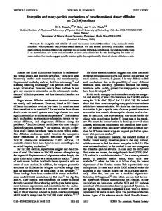
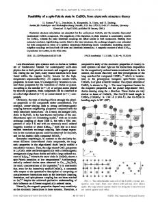
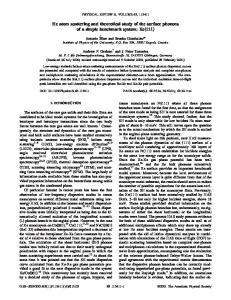
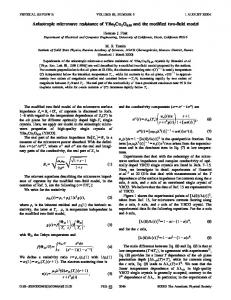
For type-II superconductors in a high magnetic field B, steady-state dissipation arises as a consequence of vortex motion. Resistive response is regulated by collective flux dynamics and pinning processes, and is characterized by the local electric field-current density (E-J) relation. Figure 1 shows a typical E-J characteristic, which is highly nonlinear in the flux creep regime J⬍J c and becomes linear in the flux-flow state JⲏJ c . This E-J constituent relation can be viewed as mesoscopic, in the sense that it describes an average response, due to many vortices, over scales greater than the characteristic pinning length 共the Larkin length1–3兲. On the other hand, the local E(J,T,B) relation does not reflect macroscopic obstructions that affect the global ¯E (J) characteristics on the scales ⰇL c . For instance, such common current-blocking obstacles as grain boundaries, microcracks, and macroscopic second-phase precipitates in hightemperature superconductors 共HTS兲 give rise to highly inhomogeneous 共often percolative兲 current distributions that have been revealed by magneto-optical imaging.4–7 These current inhomogeneities cause strong local enhancement of the electric field near macroscopic defects, which thus become a significant current-limiting factor in HTS polycrystals,8,9 and YBa2Cu3O7 共YBCO兲 coated conductors.10 This fact poses a fundamental problem of calculating the macroscopic distributions of electric field and currents, and the global E-J characteristics of inhomogeneous HTS that we regard as highly nonlinear conductors with local E-J characteristics shown in Fig. 1. In general, the relation between the global ¯E (J) and the mesoscopic E(J) characteristics can be rather complex, because of the percolative nature of current flow in HTS and the nonlinearity of the E-J relation.11–13 In this 0163-1829/2001/63共6兲/064521共26兲/$15.00

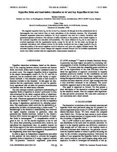
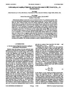
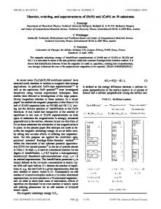
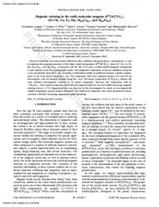
paper, we unravel the macroscopic response from the mesoscopic response by calculating exact steady-state current distributions for several key percolation structures and common circuit elements, as shown in Fig. 2. We consider here various two-dimensional 共2D兲 transport current flows in a sample connected to a dc power supply. A general method for calculating the steady-state macroscopic transport current flow is to combine the E-J relation with the static Maxwell equations “⫻E⫽0, “⫻H⫽J共 E兲 .

共1兲

A common approximation for E(J) in superconductors at J ⬍J c is the power-law form E⫽E 0 共 J/J 0 兲 n ,

共2兲

FIG. 1. E-J characteristic of a type-II superconductor. J c marks the crossover from flux creep to flux flow.

63 064521-1

©2001 The American Physical Society

MARK FRIESEN AND ALEX GUREVICH

PHYSICAL REVIEW B 63 064521

condition of current continuity, div J⫽0, provided that J ⭐J c . For a given sample geometry, these conditions can in principle be satisfied by many different transport current distributions. Such multiple solutions occur because the Bean model ignores the second Maxwell equation ⵜ⫻E⫽0, which requires the account of the nonlinear E-J characteristics 共2兲. The incorporation of the E-J material relation into Eq. 共1兲 eliminates multiple solutions of the Bean model, fixing a unique steady-state transport current distribution for given boundary conditions. Additionally, the account of E eliminates such artifacts of the Bean solutions as the infinite extent of current perturbations around local inhomogeneities and the zero thickness of the d lines. To account for the electric field induced by current flow, Eq. 共1兲 should be supplemented by the constituent relation E⫽ ␳ 共 J 兲 J. FIG. 2. Characteristic cases of nonlinear current flows solvable by the hodograph method. Darker regions mark magnetic-flux jets that represent domains of enhanced electric field. The solid and dotted lines on the percolation plot show high- and low-angle grain boundaries, respectively.

where J 0 is a current density at a particular electric-field criterion E 0 . Equation 共2兲 well describes the observed E(J) dependence over a very wide 共several decades兲 range of electric fields E, both in low-T c 共LTS兲 and high-T c superconductors, especially in the ab plane of layered Bi-based HTS.14 The power-law exponent n(T,B) depends on the temperature T and magnetic field B, and typically falls into the range 3⬍n⬍40 for HTS and 3⬍n⬍70 for LTS. One limiting case n⫽1 corresponds to the ohmic response of a superconductor above the irreversibility field B i (T). The other limiting case n→⬁ describes a stepwise function E(J), reminiscent of the critical-state model,15,16 for which E⫽0 for J⬍J c and J⫽J c E/E for E⬎0. This model has been widely used for calculations of magnetization and transport current distributions and magnetic moments of superconductors.15 In the critical-state model current flow exhibits characteristic discontinuity lines (d lines兲, along which the vector J(x,y) abruptly changes direction. In addition, finite-size defects can perturb J(x,y) over an infinite range, as it occurs in the case of magnetization current flow past a cylindrical void, for which parabolic d lines extend to infinity.16,17 Both the infinitesimal thickness of the d lines and the infinite spatial extent of current perturbations result from the assumption of zero resistivity for the idealized Bean’s E-J characteristic over the interval 0⬍J⭐J c . The above features of the critical-state model make it rather unsuitable for calculations of steady-state transport current flow around planar obstacles in Fig. 2, for which the current-carrying cross section varies along a superconductor. In the Bean model current paths break into critical-state regions with J⫽J c and subcritical regions with 0⬍J⬍J c . However the distribution of these regions depends on initial conditions 共see, e.g., Ref. 18兲 and cannot be unambiguously calculated by solving the steady-state equations div J⫽0 and J⭐J c . Thus Eq. 共1兲 for the Bean model represent an illdefined mathematical problem, which reduces to the only

共3兲

The nonlinear superconducting response is captured in the function ␳ (J), for example, ␳ ⫽ 关 J/J 0 兴 n⫺1 E 0 /J 0 for the power law E(J). Except where noted, we will assume Eq. 共2兲 for the particular calculations performed here, although the method presented in this paper works for any E-J relation determined by general models of thermally activated vortex dynamics E⬀exp关⫺U(J,T,B)/T兴. We limit our scope to the case of isotropic, 共2D兲 E-J relations. For anisotropic layered HTS, we therefore consider current flow in the ab plane with the magnetic field H储 cˆ applied along the c axis. To illustrate the complicated nature of the nonlinear Maxwell’s equations, we introduce the electrostatic potential E ⫽⫺“ ␸ and recast Eq. 共1兲 as a scalar partial differential equation “• 关 ␳ ⫺1 共兩 “ ␸ 兩兲 “ ␸ 兴 ⫽0.

共4兲

For ohmic conductors ( ␳ ⫽const), Eq. 共4兲 reduces to Laplace’s equation, for which many solution techniques exist.19,20 For the power-law E(J) relation, Eq. 共4兲 becomes “• 关兩 “ ␸ 兩 (1⫺n)/n “ ␸ 兴 ⫽0. The nonlinearity of this equation is a serious problem when calculating 共either analytically or numerically兲 distributions of electric field in superconductors, in particular, for the common restricted geometries shown in Fig. 2. The elements in Fig. 2 can also be regarded as ‘‘building blocks’’ for a more general current-blocking percolative network of high-angle grain boundaries in HTS polycrystals. For ohmic conductors, some cases shown in Fig. 2 can be solved analytically using powerful methods of conformal mapping for the complex electric potential.19,20 The nonlinearity of E(J) in superconductors does not allow one to use the theory of analytic functions, which greatly complicates the situation. Yet taking into account a realistic E(J) relation represents a principal advantage over the critical-state model, because in this case Eq. 共4兲 has a unique steady-state solution for given boundary conditions, which enables one to address dissipative processes induced by steady-state transport current flow in superconductors. Recently we have developed an analytical technique of calculation of 2D distributions of electric fields and currents in superconductors with highly nonlinear E-J characteristics.21–24 The method is based on a hodograph

064521-2

NONLINEAR CURRENT FLOW IN SUPERCONDUCTORS . . .


transformation25,26 ␸ (r)→ ␸ (E), which converts the nonlinear Eq. 共4兲 into a linear equation for ␸ (E) for any J(E). Within this hodograph representation, there are no distinctions between the linear (n⫽1) and nonlinear (n⫽1) Maxwell’s equations, therefore the same eigenfunction expansion and matrix inversion techniques previously applied to ohmic conductors can now be extended to the case of superconductors. This method proves very efficient in numerical simulations as well, allowing us to develop fast algorithms that take into account exactly both the nonlinearity of E(J) and singularities in E(x,y) near sharp edges. In previous publications we used the hodograph technique to obtain some exact solutions for dc current flows in superconductors with defects.22–24 These solutions revealed new current-flow patterns and length scales caused by the strong nonlinearity of J(E) and determined applicability limits of the critical-state model. In particular, the hodograph solutions show that current flow in superconductors generally breaks into current flow domains separated by current-domain walls of varying width, whose internal structure remains different from the well-known discontinuity lines (d lines兲6,16,28 of the Bean model even in the critical-state limit n→⬁. Another feature of nonlinear current flow in superconductors with macroscopic defects is a strong enhancement and long-range disturbances of the electric field on finite scales much larger than the defect size. The long-range disturbances of E(x,y) become crucial for restricted geometries in Fig. 2, giving rise to essential size effects that dominate the observed globaltransport properties. This paper is devoted to the detailed analysis of nonlinear current flow for restricted geometries and is organized as follows. Section II presents a qualitative discussion of characteristic length scales resulting from the highly nonlinear E(J) dependence. Section III gives a summary of the hodograph transformation technique and corresponding solutions. In Secs. IV–VII, four current-flow geometries are considered: the point source, the bridge, the current lead or elbow, and a planar defect in a film. We obtain exact solutions for the current streamlines and electric-field distributions. These are analyzed in detail, relegating technical details to the appendixes. In Sec. VIII, we consider the structures of vortex jets, current-flow domains, and domain walls, whose structure can be uncovered using the hodograph technique. Section IX is devoted to the global current-voltage characteristics and dissipation in superconductors with planar defects. In Sec. X, we conclude with a discussion.

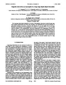
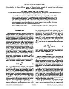
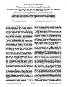
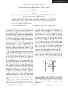
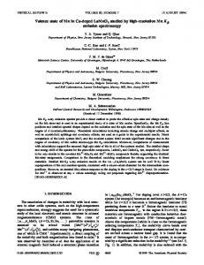
FIG. 3. Current streamlines around a planar defect in an infinite superconductor with E⫽E c (J/J c ) n , n⫽20 共Refs. 22 and 23兲共only one quadrant is shown兲. Dashed lines show the boundaries of the flux jet and stagnation region.

II. LENGTH SCALES OF VORTEX JETS IN RESTRICTED GEOMETRIES

Before analyzing exact hodograph solutions, we first discuss qualitative manifestations of the strong nonlinearity of E(J) in current flow around planar defects in infinite-size superconductors. Features of these solutions obtained in Refs. 22 and 23 will be crucial for determining nonlinear current flow in the restricted geometries in Fig. 2. Shown in Fig. 3 is a solution for the current streamlines around a planar defect of length 2a in an infinite superconductor.22,23 The nonlinearity of E(J) results in a long-range disturbance of

the electric field on scales much larger than the defect size a, in stark contrast to a short-range decay of disturbances of E(x,y) and J(x,y) on the length ⬃a in normal metals. Another distinctive feature of superconductors is the strong anisotropy of perturbations of E(x,y), which decay on very different length scales along (L 储 ) and across (L⬜ ) the direction of current flow L⬜ ⬃an, L 储 ⬃a 冑n.

共5兲

The relation L⬜ ⬃ 冑nL 储 ⰇL 储 is characteristic of superconductors in the critical state (nⰇ1).13,23 The transverse scale L⬜ can be evaluated from the following consideration. The defect blocks current flow on the length ⬃a, forcing the current aJ 0 to redistribute around the defect on the scale ⬃L⬜ . In the region x⬍L⬜ the mean current density and the electric field thus increase to J m ⬃(1⫹a/L⬜ )J 0 and E m ⬃(1⫹a/L⬜ ) n E 0 , respectively. The decay length L⬜ is defined by the condition E m ⬃E 0 , thus L⬜ ⬃na. The decay length L 储 ⬃a 冑n along current flow then follows from the general relation L⬜ ⬃ 冑nL 储 . 23 Therefore, strong (nⰇ1) nonlinearity of E(J) greatly increases the spatial scales of electric-field perturbations. Note however that E(x,y) can also vary on scales much smaller than a, as it occurs in the narrow current domain walls that replace the sharp d lines of the Bean model. As seen from Fig. 3, the disturbances of E(x,y) are mostly localized in long domains of enhanced electric field of length ⬃L⬜ and of width ⬃L 储 , sandwiched between regions ⬃L 储 of strongly depressed electric field. Because of the reflection symmetry of the current pattern in Fig. 3, only one quadrant is shown. The physical meaning of the electricfield domains in Fig. 3 becomes more transparent by consid-

064521-3



ering the distribution of vortex velocities v⫽⫺c 关 E⫻B兴 /B 2 around the defect in a strong magnetic field B when the selffield effects are negligible and the local B(x,y) equals the applied field B a . Then the elongated domains of strong electric field E(x,y)⬎1.5E 0 in Fig. 3 correspond to a channel of preferential magnetic-flux motion along the x axis. The flux is sucked from one of these electric-field domains into the edge of the defect and then gets injected from its opposite edge into the second domain, which therefore can be regarded as a magnetic-flux jet in a strongly pinned vortex structure. These jets are situated between stagnation regions of nearly motionless flux 共in Fig. 3 only one flux jet and half of the stagnation region are pictured兲. We emphasize that both the macroscopic flux jets and stagnation regions result from the geometry of current flow and the strong nonlinearity of E(J), but are not due to enhanced or reduced local flux pinning. As shown below, both the flux jets and stagnation regions are characteristic of nonlinear current flow in superconductors of restricted geometries. For instance, nonlinear current transport of polycrystals in Fig. 2 can be formulated as a percolation of magnetic flux along a discontinuous network of high-angle grain boundaries connected by vortex jets. Notice that dissipation and resistance are mostly localized within comparatively narrow vortex jets that thus become peculiar ‘‘hot spots’’ in polycrystals. Because of the large length of flux jets around defects for nⰇ1, the effects of the sample geometry in superconductors become much more pronounced than for Ohmic conductors. As an illustration, we consider a planar defect in a film of thickness d or an equivalent case of a chain of planar defects, which models faceted grain boundaries shown in Fig. 2. The length of the flux jet becomes larger than d for L⬜ ⬎d or a⬎d/n.

共6兲

If this rather weak condition is satisfied 共given typical n ⬃20–30 in HTS and 30–70 in LTS兲, then even a small defect (aⰆd) can produce a flux jet that effectively blocks the current-carrying cross section. This results in a localized voltage step at the defect and excess dissipation. The width of the flux jet L 储 can be estimated from the relation L⬜ /L 储 ⬃ 冑n, where the length of the jet L⬜ ⬃d. Hence we obtain length scales of the jet in restricted geometries L⬜ ⬃d, L 储 ⬃d/ 冑n.

E m⬃

n

共8兲

E0 .

For n⫽30, we obtain E m ⯝17.5E 0 for a 10% defect (a ⫽0.1d) and E m ⯝237E 0 for a 20% defect (a⫽0.2d). The enhancement of the electric field and dissipation in the flux jet manifests itself in a significant excess voltage ⌬V ⬃E m L 储 , ⌬V⬃

冉冊

d 冑n d⫺a

dE 0

n

.

共9兲

Another distinctive feature of the current flow observed in Fig. 3 are the regions where the nearly constant current density J⯝J c sharply changes direction. These orientational current-flow domains are separated by comparatively narrow current-domain walls, reminiscent of the d lines between regions of different critical-flow orientation in the Bean model. However, there are important differences between the current domain walls described by exact solutions of the Maxwell equations and the phenomenological d lines. First of all, the current domain walls have an internal structure and a varying width ⬃d/ 冑n, which depends both on the n value and the geometry of current flow. For instance, for current flow past a planar defect in Fig. 3, the width of the current domain walls increases with the distance from the defect. It is the broadening of the domain walls that provides the decay of current perturbations on a finite length L⬜ ⬃an.22,23 Moreover, the current domain walls described by exact hodograph solutions remain different from the d lines even in the critical-state limit n→⬁, for which the current flow near domain walls exhibits no discontinuities in the tangentional components of J(x,y) and E(x,y). The spatial scales of the orientational current-flow domains for the infinite geometry in Fig. 3 are of the order L⬜ ⬃an. As shown below, the sizes of these orientational domains for restricted geometries become of the order of the sample dimension d both along and across current flow. We conclude this section with a brief discussion of the transient time scales t 0 , on which the steady-state transport current distributions set in after the dc power supply was turned on.23 The time constant t 0 is determined by magneticflux diffusion and is inversely proportional to a final dc electric field E 0 in a superconductor27

共7兲

The strong nonlinearity of E(J) results in a peculiar ‘‘pinch effect,’’ manifesting itself as a contraction of the flux jet as n increases. In the critical-state limit n→⬁ the jet turns into a line. The contraction of the vortex jet with increasing n is accompanied by a strong increase of vortex velocities and thus electric field E(x,y) in the jet as compared to the electric E 0 for the uniform current flow far away from the defect 兩 x 兩 Ⰷd/ 冑n. This follows from the current-continuity condition J 0 d⯝J m (d⫺a), where J m and E m ⫽E 0 (J m /J 0 ) n are the current density and the electric field in the jet on the side of the film opposite to the defect. Hence,

冉冊 d d⫺a

t 0 ⬃ ␮ 0 sJ c L 2 /E 0 ,

共10兲

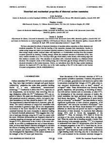
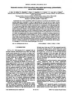
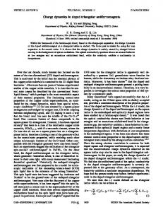
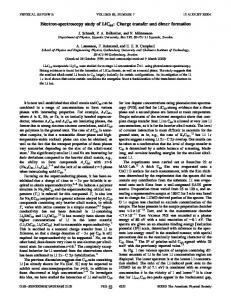
where L is a characteristic sample size 共thickness or width兲, J c is the critical current density, and s⫽ ⳵ ln J/⳵ ln t is the dimensionless flux creep rate. For the power-law E-J relation, we have s⫽1/(n⫺1).3 We illustrate Eq. 共10兲 for a planar defect in a film, for which the transient time evolution of the current flow is sketched in Fig. 4. Here Fig. 4共a兲 shows an initial distribution J(x,y) in which the white region carries no current, while the shaded upper part of the sample cross section is in a critical state and carries the current density J m ⫽I/(d⫺a), where I is the total fixed current. This unrelaxed current configuration has an infinite stagnation region 共white兲 and is consistent with the Bean model. However

064521-4



Unless specially noted, we consider in this paper a true steady-state current flow (tⰇt 0 ), thus neglecting the transient relaxation. Detailed numerical analysis of nonlinear flux diffusion in superconductors in ac magnetic fields have been performed by Brandt.28 III. HODOGRAPH TRANSFORMATION A. Formalism

In this work we consider a superconductor in a strong magnetic field B a ⰇB p ⬃ ␮ 0 dJ c , so that self-field and demagnetization effects are negligible.29–31 Then the constituent relation E⫽ ␳ (B,J)J, which generally depends on the local B(x,y), especially for B⬍B p , can be replaced by the relation E⫽ ␳ (B a ,J)J, which is independent of B. In this case the 2D distribution J(x,y) can be calculated by introducing the electric potential ␸ and the stream function ␺ : E⫽⫺“ ␸ , J⫽“ ␺ ⫻zˆ , “•J⫽0.

FIG. 4. Evolution of transport current distribution for a film with a crack toward the steady state after switching on the dc power supply. Different shades of gray quantify magnitudes of electric field 共in three-level scale兲, and arrows show the direction and magnitude of local current density J. 共a兲 shows initial unrelaxed state of nearly constant J above the crack. 共b兲 shows a transient state, for which magnetic-flux diffusion tends to make the electric field more uniform across the sample, and the stagnation region and the flux jet are formed. 共c兲 shows the final dc state, which is a cartoon of an exact hodograph solution obtained in Sec. VII. Here the darkest and the white areas mark the magnetic-flux jet and the stagnation region, respectively.

the finite resistivity at J⬍J c causes diffusion of the stepwise electric field E(y) in Fig. 4共a兲 and its evolution toward the uniform final steady-state distribution of E 0 ⫽E c (I/dJ c ) n across the sample far away from the defect. As a result, the stagnation region shrinks as shown in Fig. 4, converging to a steady-state size ⬃d for t⬎t 0 , where the time t 0 is determined by magnetic-flux diffusion across the sample. The diffusion time t 0 ⬃L 2 /D m is then given by Eq. 共10兲, where L ⬃a is the diffusion distance, and D m ⬃ ␮ 0 J c /nE is a nonlinear diffusivity of the electric field. The steady-state condition tⰇt 0 was discussed in detail in Ref. 23 for different geometries including those in Fig. 2. It was shown that for electric fields E 0 ⬃1 ␮ V/cm characteristic of transport measurements, and sample sizes L⬃10⫺3 ⫺1 cm, the relaxation-time constant t 0 ⬃10⫺3 ⫺10 s is much shorter than the typical experimental time window.

共11兲

The contours of the function ␺ (x,y)⫽const point in the direction of local current flow, and their density is proportional to the local current density. In Ohmic conductors, both ␸ and ␺ satisfy the Laplace equations ⵜ 2 ␸ ⫽0, ⵜ 2 ␺ ⫽0. This fact enables one to introduce the complex potential w(z)⫽ ␸ ⫺i ␳ ␺ as an analytic function of the complex coordinate z ⫽x⫹iy, obtaining various exact solutions for the 2D current flow.19,20 For superconductors (n⬎1), the potential w(z) satisfies a highly nonlinear partial differential equation and is no longer an analytic function. However, we can apply the hodograph transformation,25,26 which linearizes the equation for w(x,y) by changing variables from the Cartesian coordinates x and y to J and ␪ 共or, equivalently, E and ␪ ). The amplitude of the current density J(x,y) and the corresponding flow angle ␪ (x,y) are defined through the relation Je i ␪ ⫽J x ⫹iJ y . To show how the hodograph transformation works, we write Eqs. 共1兲 or 共11兲 in the differential form d ␸ ⫽⫺E x dx⫺E y dy, ␳ d ␺ ⫽E y dx⫺E x dy,

共12兲

where ␳ (E)⫽E/J. Equation 共12兲 can be combined in a single complex equation d ␸ ⫺i ␳ d ␺ ⫽⫺Ee ⫺i ␪ dz, thus

⳵ E z⫽⫺e i ␪ 共 ⳵ E ␸ ⫺i ␳⳵ E ␺ 兲 /E,

共13兲

⳵ ␪ z⫽⫺e i ␪ 共 ⳵ ␪ ␸ ⫺i ␳⳵ ␪ ␺ 兲 /E,

共14兲

where ␴ (E)⫽ ⳵ J/ ⳵ E is the differential conductivity and ⳵ ␣ ⬅ ⳵ / ⳵ ␣ . The condition ⳵ ␪2 E z⫽ ⳵ E2 ␪ z gives the following relations between partial derivatives of ␺ and ␸ :

⳵ ␪ ␸ ⫽⫺ 共 E 2 /J 兲 ⳵ E ␺ , ⳵ E ␸ ⫽ 共 E ␴ /J 2 兲 ⳵ ␪ ␺ .

共15兲

Equating the mixed derivatives ⳵ ␪2 E ⫽ ⳵ E2 ␪ for ␺ and ␸ , we obtain the following linear equations for ␺ and ␸ valid for any nonlinear dependence J(E):

064521-5

␴ E ⳵ 2␺ J2 ⳵␪

⫹ 2

冉冊

⳵ E2 ⳵␺ ⫽0, ⳵E J ⳵E

共16兲


J ⳵ 2␸ E2 ⳵␪

⫹ 2

冉


冊

⳵ J 2 ⳵␸ ⫽0. ⳵E ␴E ⳵E

共17兲

Equations 共16兲 and 共17兲 simplify considerably for the power law E(J), giving32 J 2 ⳵ 2␺ ⳵ ␺ ⳵ 2␺ ⫹J ⫽0, ⫹ n ⳵J2 ⳵J ⳵␪2

⳵ 2␸

nE 2

⳵E

⫹E 2

共18兲

⳵␸ ⳵ 2 ␸ ⫽0. ⫹ ⳵E ⳵␪2

共19兲

In Eq. 共18兲 we can change variables E⫽E 0 (J/J 0 ) n to express ␺ (E, ␪ ) as a function of the electric field E. This representation will be convenient later on when calculating 2D distributions of E(x,y). Equations 共18兲 and 共19兲 can be solved by the separation of variables of the form22,23

冉冊

␺ 共 J, ␪ 兲 J ⫽A 0 ⫹ 共 B 0 ⫹D 0 ␪ 兲 I J0 ⬁

⫹

兺 Cm m⫽1 ⬁

⫹

兺

m⫽1

Dm

冉冊冉冊 J J0

⫹ ␶m

J J0

⫺ ␶m

1⫺n

⫹C 0 ␪

sin共 m ␪ ⫹ ␾ m 兲 sin共 m ␪ ⫹ ␻ m 兲 .

共20兲

共21兲

The total current I and the average sheet current density J 0 ⫽I/d, where d is the sample width are natural scales for ␺ and J, adopted throughout this work. As described in Refs. 22 and 23, Eqs. 共13兲–共15兲 can be used to perform the inverse transformation from the hodograph to physical coordinates, which yields

冉冊

⫺n

兵 iB 0 共 n⫺1 兲

⫹D 0 关 1⫹i 共 n⫺1 兲 ␪ 兴其 ⬁

⫺e

i␪

兺

m⫽1

Cm

冉冊

J ⫹ ␶ m ⫺1 J 0

⫹ ␶m ⫺1

关 m cos共 m ␪ ⫹ ␾ m 兲

⫹ ⫺i ␶ m sin共 m ␪ ⫹ ␾ m 兲兴 ⬁

⫺e

i␪

兺

m⫽1

Dm

冉冊

J ⫺ J ␶ m ⫺1 0

⫺ ⫺i ␶ m sin共 m ␪ ⫹ ␻ m 兲兴 .

⫺ ␶m ⫺1

fore reduced to determining these expansion coefficients for particular boundary conditions. B. Boundary conditions

1 ␶ m⫾ ⫽ 关 1⫺n⫾ 冑共 n⫺1 兲 2 ⫹4nm 2 兴 . 2

J 0 e i␪ J z 共 J, ␪ 兲 ⫽F 0 ⫹C 0 e i ␪ ⫹ d J n J0

FIG. 5. Crack in film geometry. 共a兲 Physical representation with boundary conditions ␺ 兩 AB ⫽ ␺ 兩 BC ⫽I and ⳵ y ␺ 兩 CD ⫽ ␺ 兩 DE ⫽0. 共b兲 Periodic extension for a chain of planar defects or a faceted grain boundary. Here the light gray area marks orientational current-flow domains, while the dark gray marks the flux jets of a strongly enhanced electric field.

关 m cos共 m ␪ ⫹ ␻ m 兲

共22兲

Equations 共20兲 and 共22兲 constitute a complete family of exact solutions for isotropic 2D current flows. The solutions for ␺ (J, ␪ ) and z(J, ␪ ) are expressed parametrically, in terms of the hodograph variables J and ␪ and expansion coefficients A 0 , B 0 , C m , D m , F 0 , ␾ m , and ␻ m . The problem is there-

The utility of the hodograph transformation rests on two criteria. The first one is that the Maxwell equations become linear in the hodograph representation. The second criterion is equally important: the transformed boundary conditions 共BC兲 in the hodograph plane must be simple enough to enable analytical solutions. In general, the hodograph transformation results in highly nonlinear BC’s for current flow around curved boundaries.21,23 However there is a wide class of physical problems like those shown in Fig. 2 for which the BC’s remain linear, which enables us to obtain exact solutions for nonlinear current flows. The eigenfunction expansions given in Eqs. 共20兲 and 共22兲 are particularly convenient for the following BC in the physical plane. First, the sample edges should be straight to ensure that the current, flowing tangentially along the sample boundary, is represented by a constant flow angle ␪ 0 . The transformed BC then corresponds to a straight line ␪ ⫽ ␪ 0 in the hodograph plane. Second, the angles inscribed inside sample corners should be rational fractions of 2 ␲ ; this produces zeros of the eigenfunctions at appropriate values of ␪ . This latter restriction is not severe, since other eigenfunction expansions are readily obtained for different angular configurations. To illustrate these BC’s, we consider a planar defect in a film, for which a detailed solution is given in Sec. VII. The physical representation of this geometry is shown in Fig. 5共a兲. Current flowing through a channel is blocked by an unpenetrable wall BC forcing the current to pass through an aperture CD. Far away from the constriction, the flow becomes uniform, with current density J 0 . At point D, the current density reaches a value J m . The current density possesses a singularity at point C and a stagnation point B, where the current density drops to zero. Because of symmetry, we only need to solve one half of the flow problem 共top half兲. We make point D the origin of the physical plane. A and E represent asymptotic points far from the constriction.

064521-6



FIG. 7. Point source inside a 90° corner. 共a兲 Physical representation with streamlines. Point source is located at origin, with boundary conditions ␺ ⫽0 共vertical boundary兲 and ␺ ⫽I 共horizontal boundary兲. 共b兲 Hodograph representation.

FIG. 6. 共a兲 Hodograph representation of constriction geometry in Fig. 5共a兲 for the upper half of the physical plane. Boundary conditions are given in parentheses. 共b兲 Hodograph representation of constriction geometry for n→⬁.

Along any wall, the normal component of J must vanish. Equation 共11兲 indicates that the stream function will be constant along such a boundary. Since ␺ (x,y) contains an arbitrary additive constant, we choose ␺ 兩 DE ⫽0 along the line DE. Then along the boundary ABC, we set ␺ 兩 ABC ⫽I, as consistent with a total current I. Along the symmetry line CD, the tangential component of J vanishes, thus ⳵ y ␺ 兩 CD ⫽ ⳵ ␪ ␺ 兩 CD ⫽0. Because of the simplicity of the BC in the physical plane, points A, B, C, D, and E can be mapped immediately onto the hodograph plane, as demonstrated in Fig. 6. Current flow along the lines AB, CD, and DE is characterized by ␪ ⫽ ␲ /2, while flow along BC corresponds to ␪ ⫽ ␲ . At points B and C, the current ‘‘turns a corner.’’ These two points are mapped onto lines in the hodograph plane: J⫽0 and J⫽⬁, respectively. The characteristic current scales J 0 and J m naturally divide the hodograph plane in Fig. 6 into three regions with distinct BC. The lines separating these regions 共e.g., J⫽J 0 ) have no special significance in the physical plane. We therefore enforce the following continuity conditions at J⫽J 0 and J⫽J m :

␺ (1) 共 J 0 兲 ⫽ ␺ (2) 共 J 0 兲 , ⳵ J ␺ (1) 共 J 0 兲 ⫽ ⳵ J ␺ (2) 共 J 0 兲 ,

共23兲

where ␺ (1) and ␺ (2) represent the stream-function solutions in adjoining regions. These are solved by Fourier analysis in terms of the variable ␪ . In this way, the matching conditions 共23兲 give the equations for the hodograph expansion coefficients, which can be expressed in the standard matrix form

兺

IV. POINT SOURCE

An instructive geometry is the point source flowing into an infinite plane. This case models a current lead attached to the film surface, or the Corbino-disk geometry used for studies of vortex dynamics in HTS.33 From symmetry considerations, it is sufficient to consider a point source located at the origin flowing into a single quadrant, as shown in Fig. 7共a兲. The lines x⫽0 and y⫽0 then form sample boundaries. Because of radial symmetry, the point-source geometry can be solved in Cartesian coordinates for any nonlinear E(J). We consider the radial coordinates r and ␪ , defined as re i ␪ ⫽z ⫽x⫹iy. The total current I flowing across the quarter-circle arc r⫽const is given by I⫽ ␲ rJ/2, thus J⫽

2I rˆ. ␲r

共25兲

From Eq. 共11兲, we obtain “ ␺ ⫽(2I/ ␲ r) ␪ˆ , whence ␺ ⫽2I ␪ / ␲ ⫹const. The formulas of this section can be used for the Corbino disk by replacing I→I/4. It is illuminating to reproduce these results using the hodograph transformation. The values of ␺ on the vertical and horizontal sample boundaries are constants given by ␺ ⫽0 and I, respectively, as shown in Fig. 7共b兲. In this case all coefficients C m and D m except C 0 and A 0 in the general solution 共20兲 vanish. We therefore associate a nonzero value of C 0 with point-source behavior, which often appears in more complicated geometries, as shown below. The boundary requirements are met by the solution A 0 ⫽⫺1, C 0 ⫽2/␲ , or

␺ ⫽⫺I⫹2I ␪ / ␲ .

共26兲

From Eq. 共22兲 with J 0 d⫽I, we arrive at the solution

⬁

m ⬘ ⫽1

tained by matrix inversion of Eq. 共24兲 either analytically or numerically using any of the well-developed and fast algorithms.

K m,m ⬘ •C m ⬘ ⫽G m ,

共24兲

where C m represents the expansion coefficients in all the different hodograph regions. Thus, the values C m can be ob-

z⫽e i ␪

2I , ␲J

which is equivalent to Eq. 共25兲.

064521-7

共27兲



FIG. 8. Bridge geometry. 共a兲 Physical representation. Boundary conditions are given by ␺ ⫽I along left sample boundary 共solid line兲 and ␺ ⫽0 along center line 共dashed兲. 共b兲 Hodograph representation, corresponding to left half of physical plane.

Equations 共26兲 and 共27兲 result from the current conservation and radial symmetry, thus they are independent of the form of E(J). We can exploit this situation to derive results that are not easily obtained in other geometries. For example, since J becomes singular at the point source, a circular fluxflow domain is nucleated around the origin. If the flux flow occurs when J(r) exceeds a critical current density J c , the domain radius is given by r c ⫽2I/ ␲ J c . Assuming a relation E⯝ ␳ F (J⫺J c ) within the flux-flow domain, the resulting dissipation is given by Q⫽

冕

E•J d 2 r⯝

冋冉

冊

册

2I 2 ␳ F 2I ␲ bJ c ln ⫹ . ␲ ␲ ebJ c 2I

共28兲

A flux-flow region thus surrounds a small current lead of radius b⬍r c . As shown in the following sections, current flowing around a sharp corner also induces flux-flow domains. V. BRIDGE

The bridge geometry, pictured in Fig. 8共a兲, is quite common in transport experiments. By symmetry, it is only necessary to solve for half of the current distribution; we focus on the left half. The dashed reflection line at the center is taken as a sample boundary. Along this line the stream function is a constant, and we set ␺ ⫽0. Along the other boundary, we have ␺ ⫽I. In contrast to the point source, the bridge geometry has a characteristic length scale b 共the bridge width兲, and a current-density scale J 0 ⫽I/b, corresponding to uniform current flow in the channel, far from the opening (yⰆ⫺b). The point source corresponds to the limit b→0. As shown in Fig. 8共b兲, the hodograph plane consists of two regions separated by the line J⫽J 0 . The solutions for current flow through the bridge are given in Appendix B, including exact expressions for the hodograph coefficients in Eqs. 共20兲 and 共22兲. Current streamlines are shown in Fig. 9 for an ohmic conductor (n⫽1) 共a兲 and a superconductor with n⫽30 共b兲.34 Similar asymptotic behaviors are observed in the two plots. In the upper-half plane, the asymptotic flow, far from the channel opening, is point-source-like, with the apparent point source located at the origin. Mathematically, the source of this behavior is in the term 2 ␪ / ␲ in Eq. 共B1兲 and the corresponding term (2e i ␪ / ␲ )J/J 0 in Eq. 共B3兲. When

FIG. 9. Calculated current streamlines for bridge geometry. 共a兲 n⫽1. 共b兲 n⫽30.

J→0, these terms dominate, and we recover the point-source solutions of Sec. IV. In the lower-half plane, far from the opening, the current approaches its asymptotic uniform behavior: J⫽J 0 yˆ. As follows from Fig. 9, for the normal metal, the transition between the different asymptotic regimes is rather gradual, while for a superconductor (nⰇ1), the transition is much sharper and occurs mainly near the channel opening. We now use the general formulas of Appendix B to calculate distributions of J(x,y) and E(x,y) along the sample surface and the central line x⫽0. Along the vertical sample edge, adjacent to the corner x⫽⫺b, we have ␪ ⫽ ␲ /2 and J ⬎J 0 . Then Eq. 共B4兲 gives J(y) in the form 4b y⫽⫺ ␲

⬁

兺

m⫽1

⫹ ␶ 2m

冉冊

J ⫺ ⫹ ⫺ 共 ␶ 2m ⫺ ␶ 2m 兲共 ␶ 2m ⫺1 兲 J 0

⫺ ␶ 2m ⫺1

,

共29兲

⫾ are given by Eq. 共21兲. where ␶ 2m The compression of current streamlines near the corner results in singularities of E(x,y) and J(x,y), which may produce local flux-flow behavior. Very near the corner, where J→⬁, the lowest-order term with m⫽1 in Eq. 共29兲 dominates the sum, giving ⫺

⫺

J⬀ 兩 z⫹b 兩 1/( ␶ 2 ⫺1) , E⬀ 兩 z⫹b 兩 n/( ␶ 2 ⫺1) .

共30兲

These results are valid when approaching the singular point from any direction. When n⫽1 we obtain J⬀E⬀ 兩 x⫹iy ⫹b 兩 ⫺1/3, while for nⰇ1, we have J⬀ 兩 x⫹iy⫹b 兩 ⫺1/n and E ⬀1/兩 x⫹iy⫹b 兩 . As n grows, the singularity in the current density becomes weaker, vanishing as n→⬁. In this limit,

064521-8



the current density becomes uniform below the channel opening 共line y⫽0), such that J⫽J 0 yˆ. However the singularity in the electric field is enhanced for large n as compared to n⫽1. Similar large-n singular behavior was observed previously in Refs. 22 and 23, for current flow past a small planar defect. This behavior is a general feature of flow past a sharp corner for any angle. For finite n, the current density approaches its asymptotic uniform value J 0 , slightly below the channel opening (yⱗ ⫺b). In this ‘‘tail’’ region, we have J 0 ⫺J(y)ⰆJ 0 , so the convergence of the sum in Eq. 共29兲 is determined by the ⫾ from Eq. region mⰇ1. Taking large-m asymptotics of ␶ 2m 共21兲, we rewrite Eq. 共29兲 as ⬁

y⯝W n ⫺

兺

b 共 J 0 /J 兲 2m 冑n

␲ 冑nm

m⫽1

⫽W n ⫹l b ln关 1⫺ 共 J 0 /J 兲 2 冑n 兴 ,

共31兲

thus J⯝J 0 ⫹

J0 2 冑n

共32兲

e (y⫺W n )/l b .

The decay length l b and the shift W n are given by

⬁

W n ⫽⫺b

兺 m⫽1

冋

l b ⫽b/ ␲ 冑n, ⫹ 4 ␶ 2m ⫺ ⫹ ⫺ ␲ 共 ␶ 2m ⫺ ␶ 2m ⫺1 兲兲共 ␶ 2m

⫺

1

␲ 冑nm

册

共33兲 . 共34兲

The value W n is weakly n dependent. The length l b is similar to the characteristic scale L 储 in Eq. 共7兲. When n→⬁, the tail disappears (l b →0), so that J⫽J 0 for all y⬍0. Now we calculate J(x) along the horizontal sample edge, adjacent to the corner, where x⬍⫺b, y⫽0. Away from the small 共for nⰇ1) singular region near the corner, the current density falls into the range J⬍J 0 , with a current-flow angle ␪ ⫽ ␲ . In this case the distribution J(x) is obtained from Eq. 共B3兲 in the form ⫹

⬁

⫺ 4b 共 ⫺1 兲 m ␶ 2m 共 J/J 0 兲 ␶ 2m ⫺1 2I ⫹ . x⫽⫺ ⫺ ⫹ ⫹ ␲ J m⫽1 ␲ 共 ␶ 2m ⫺ ␶ 2m ⫺1 兲兲共 ␶ 2m

兺

共35兲

Far away from the bridge, where JⰆJ 0 , the first 共pointsource兲 term dominates, giving x⯝⫺2I/ ␲ J. Corrections to this description correspond to leading-order terms in the summation. Now we calculate the electric-field distribution along the central line x⫽0, where ␪ ⫽ ␲ /2 and J⬍J 0 . From Eq. 共B3兲 we obtain the following relation for the distribution y(E):

冉冊

2b E y⫽ ␲ E0

⬁

⫺1/n

⫺

FIG. 10. Bridge characteristics. 共a兲 Electric-field distribution along center line. 共b兲 Excess voltage (⌬V) vs n.

asymptotic uniform flow state E⯝E 0 . Equation 共32兲 describes the behavior of the tail in this region with a modified W n . For yⲏ0, the electric field converges to its asymptotic point-source behavior E⯝E 0 (2b/ ␲ y) n . Near the opening, where y⯝0, E crosses over between these two asymptotic regimes. In this vicinity, E is also affected by the nearby corner singularity. We use Eq. 共36兲 to calculate the excess voltage ⌬V⬅V ⫺E 0 L, defined as the difference between the total voltage signal and the assumed voltage drop along the bridge. This addresses a common situation in transport measurements, where the edge singularities and nonuniform distribution of E(x,y) near the bridge opening are not taken into account by the conventional interpretation, which assumes a uniform distribution E(x,y)⫽E 0 inside the bridge (y⬍0) and E(x,y)⫽0 for y⬎0. To calculate the ⌬V, we consider two current leads attached to either side of the sample, along the center 共mirror兲 line x⫽0 关see Fig. 8共a兲兴. For simplicity, the leads are placed at an infinite distance from the bridge element (y→⫾⬁). We assume that the bridge is long enough that the two openings do not interact. The excess voltage ⌬V is obtained from the integral ⌬V⫽2

⫹

⫺ 4b ␶ 2m 共 E/E 0 兲 ( ␶ 2m ⫺1)/n

兺 ⫺ ⫹ 兲共 ␶ ⫹ ⫺1 兲 . m⫽1 ␲ 共 ␶ ⫺ ␶ 2m

2m

共36兲

⫽2

2m

Results for E(y) obtained from Eq. 共36兲 are shown in Fig. 10共a兲. For yⱗ0, the electric field quickly attains its

冕冕

0

⫺⬁ E1

E0

共 E⫺E 0 兲 dy⫹2

共 E⫺E 0 兲

冕

⬁

E dy

0

⳵y dE⫹2 ⳵E

冕

0

E1

E

⳵y dE, ⳵E

共37兲

where the function y(J) is given by Eq. 共36兲, E 1 is the value of E, for which y(E 1 )⫽0, and the factor 2 accounts for two

064521-9



FIG. 11. Current-lead or elbow geometry. 共a兲 Physical representation, with boundary conditions ␺ ⫽I 共lower and left sample edges兲 and ␺ ⫽0 共upper and right sample edges兲. 共b兲 Hodograph representation.

ends of the bridge. We may also express ⌬V in terms of an effective excess length ⌬L⬅⌬V/E 0 , which represents the length of a bridge element needed to produce the same excess voltage signal ⌬V, assuming a uniform electric field E 0 . In Fig. 10共a兲, the excess length ⌬L is shown for n⫽30. The excess voltage ⌬V as a function of n is shown in Fig. 10共b兲. The rapid drop off of the electric field for point-source flow (E⬀y ⫺n ) causes ⌬L and ⌬V to decrease with increasing n. For n→1, the slower drop off E⬀1/y produces a logarithmic singularity in the voltage integral, Eq. 共37兲. For the bridge geometry, the ohmic case is thus particularly sensitive to the placement of voltage taps. VI. CURRENT LEAD

The current-lead or elbow geometry is shown in Fig. 11共a兲, which also describes the flux transformer configuration.35 The current lead contains two currentdensity scales J 1 ⫽I/d and J 2 ⫽I/b, which correspond to current flow in the large and small channels, far away from the corner. The anisotropy parameter is defined as r⬅b/d, with 0⬍r⭐1. The hodograph plane of the elbow geometry consists of three regions, separated by the lines J⫽J 1 and J⫽J 2 , as shown in Fig. 11共b兲. This problem is more complicated than that for the bridge, since it involves an additional hodograph region. Nevertheless, the current-lead geometry can be solved exactly, as shown in Appendix C. Several limiting cases can be identified. The case r ⫽b/d⫽J 1 /J 2 ⫽1 corresponds to a symmetric elbow, for which the hodograph region 共2兲 vanishes. In a different limit, we take the upper film edge to infinity (d→⬁, r→0) to obtain the bridge geometry. Since the current density J 1 then goes to zero, the lower hodograph region 共1兲共with 0⭐J ⭐J 1 ) disappears. Region 共2兲 is now bordered by the line J (2) to zero in order to keep ⫽0, and we set the coefficients D 2m the stream function finite. In this way, we recover the bridge solution of Sec. V and Appendix B. Current streamlines for the elbow geometry are shown in

FIG. 12. Current streamlines for an asymmetric elbow, with r ⬅b/d⫽0.15. 共a兲 Ohmic conductor, n⫽1. 共b兲 Superconductor, n ⫽30. Dashed line 关Eq. 共58兲兴 shows approximate d line. Shaded area marks main region of nonuniform flow: a rectangle of size W ⬁ ⫻d.

Fig. 12. For n⯝1, the streamlines are compressed near the corner, and a singularity appears in some region very near the corner. As n increases, the singular region shrinks in size, vanishing in the limit n→⬁. More remarkably, current flow breaks up into characteristic flow domains, including uniform flow domains, where J⯝const, and a point-source flow domain, for which J⬀1/兩 z 兩 . This point-source behavior originates primarily in hodograph region 共2兲, whose solution contains the leading terms proportional to C 0 in Eqs. 共20兲 and 共22兲. By contrast, such orientational flow domains do not occur in normal conductors, where streamlines turn smoothly around the corner. We use the exact solution of Appendix C to calculate electric field and current-density distributions E(x) and J(x) along the bottom and top edges of the main channel. These distributions are of prime interest in flux transformer experiments in which voltage taps are placed along ‘‘primary’’ 共bottom兲 and ‘‘secondary’’ 共top兲 edges, respectively. Along the primary edge 共see inset of Fig. 13兲 we have J⬎J 1 . Very near the singular point (x⫹iy⫽⫺b) we enter the highcurrent regime J⬎J 2 ⬎J 1 . Since ␪ ⫽ ␲ along the primary line, Eq. 共C6兲 gives J(x) in the form

064521-10

⬁

x⫽⫺b⫹

兺

m⫽1

⫺

冉冊

⫹ 4b ␶ 2m 关共 ⫺1 兲 m ⫺r ⫺ ␶ 2m 兴 J ⫺ ⫹ ⫺ ␲ 共 ␶ 2m ⫺ ␶ 2m ⫺1 兲 J 2 兲共 ␶ 2m

⫺ ␶ 2m ⫺1

. 共38兲



The exponential convergence of the electric field over the length l e ⬃d/ 冑n is characteristic of confined geometries, as discussed in Sec. II. We contrast this result with the radial current flow in the upper half of the bridge geometry in Fig. 9, for which asymptotic convergence to point-source flow away from the origin occurred as a power law. The second length scale W n has particular physical significance for n →⬁, when ⬁

2

4d 共 ⫺1 兲 m 共 b/d 兲 4m 2d . W ⬁⫽ ⫺ ␲ m⫽1 ␲ 共 4m 2 ⫺1 兲

兺

FIG. 13. Transformer geometry with r⬅b/d⫽0.1 共inset兲. Electric-field distributions along primary (E⬎E 1 ) and secondary (E⬍E 1 ) edges for different exponents n 共right to left兲: n⫽3 共solid兲, 30 共dashed兲, 300 共dot dashed兲, and ⬁ 共dotted兲.

Approaching the corner, the current and field distributions are dominated by the leading-order term with m⫽1, giving the same singularities 共30兲 in E(x,y) and J(x,y) as for the bridge. In the limit n→⬁, the current density at the corner does not diverge at all, but reaches a maximum value of J 2 . Away from the singularity, where J⭐J 2 , Eq. 共C5兲 gives J(x) along the primary edge

冉冊

⬁

⫹ 4 d ␶ 2m 2I J x⫽⫺ ⫺ ⫺ ⫹ ⫺ ␲ J m⫽1 ␲ 共 ␶ 2m ⫺ ␶ 2m 兲共 ␶ 2m ⫺1 兲 J 1

兺

⬁

⫹

兺 m⫽1

冉冊

⫺ 4b ␶ 2m 共 ⫺1 兲 m

J ⫺ ⫹ ⫹ ␲ 共 ␶ 2m ⫺ ␶ 2m 兲共 ␶ 2m ⫺1 兲 J 2

.

⬁

x⫽

⬁

冑nE 1 2

e (x⫹W n )/l e , l e ⫽

冋

d

␲ 冑n

,

共39兲

共40兲

⫹ 4 d ␶ 2m 2d d ⫺ W n⫽ ⫹ ⫺ ⫹ ⫺ ␲ m⫽1 ␲ 共 ␶ 2m ⫺ ␶ 2m 兲共 ␶ 2m ⫺1 兲 ␲ 冑nm

兺

⫹

⫺

⫺ 4 d ␶ 2m 共 ⫺1 兲 m r ␶ 2m ⫺ ⫹ ⫹ ␲ 共 ␶ 2m ⫺ ␶ 2m ⫺1 兲兲共 ␶ 2m

册

.

兺

m⫽1

Resulting distributions for E(x) are shown in Fig. 13. For the asymmetric elbow shown in Fig. 12 with r⫽J 1 /J 2 ⬍0.5, there is an intermediate region J 1 ⱗJⱗJ 2 , where the first term on the right-hand side in Eq. 共39兲 dominates, producing point-source-like behavior. For a more symmetric elbow with r⭓0.5 or for n⯝1, no clear point-source behavior is observed 关Fig. 12共a兲兴. Far away from the current lead xⰆ⫺b, where J⯝J 1 , the distribution x(E) given by Eq. 共39兲, is determined by the terms with mⰇ1. In this case we can set J⯝J 1 in the second sum in Eq. 共39兲 and replace the first summation by integration as we did to obtain Eq. 共32兲. This yields E⯝E 1 ⫹

For b/d⬍0.88, the series may be truncated at one or two terms with excellent accuracy, giving W ⬁ ⯝2d/ ␲ if bⰆd. For b/d⬎0.88, we can set b/d→1 in Eq. 共42兲, obtaining W ⬁ →d after summation. The meaning of W ⬁ can be understood as follows. For nⰇ1, the electric field converges rapidly to its asymptotic value E 1 , away from the corner. As n→⬁, the decay length l e →0 vanishes, and the perturbations of the electric-field perturbations disappear in the regions 兩 x 兩 ⭓W ⬁ , where the uniform flow state sets in: E⫽⫺E 1 yˆ. For finite n, the electric field becomes nonuniform, and W ⬁ marks the onset of the exponential decay of the electric-field disturbance. The main disturbance in E(x,y) therefore occurs in a rectangle W ⬁ ⫻d, as shown in Fig. 12共b兲. Next, we investigate the electric field and current distributions along the secondary sample edge. Along this line we have J⬍J 1 and ␪ ⫽ ␲ . Thus Eq. 共C4兲 gives

⫺ ␶ 2m ⫺1

⫹ ␶ 2m ⫺1

共41兲

共42兲

⫹

冉冊

⫺ 4 d ␶ 2m 关 ⫺1⫹ 共 ⫺1 兲 m r ␶ 2m 兴 J ⫺ ⫹ ⫹ ␲ 共 ␶ 2m ⫺ ␶ 2m ⫺1 兲 J 1 兲共 ␶ 2m

⫹ ␶ 2m ⫺1

.

共43兲

Near the stagnation point (x⫹iy⫽id), where the electric field vanishes, the term with m⫽1 in Eq. 共43兲 dominates, giving ⫹

E⬀ 兩 x⫹iy⫺id 兩 n/( ␶ 2 ⫺1) .

共44兲

When n⫽1, we have J⬀E⬀ 兩 x⫹iy⫺id 兩 , while for nⰇ1 we obtain J⬀ 兩 x⫹iy⫺id 兩 1/3 and E⬀ 兩 x⫹iy⫺id 兩 n/3. Distributions of E(x) along the secondary edge given by Eq. 共43兲 are shown in Fig. 13. For nⰇ1, the electric field drops exponentially at x⬍⫺W n , converging to a step function at x⫽⫺W ⬁ when n→⬁. In the tail region (xⱗ⫺W ⬁ ), where E⯝E 1 , Eq. 共43兲 can be estimated using the same techniques that led to Eq. 共40兲 for the primary edge. We obtain exactly the same result, but with a new expression for W n . In the limit n→⬁, this reduces to the previous expression for W ⬁ , as given in Eq. 共42兲. Using Eqs. 共39兲 and 共43兲, we can compute quantities of interest for the flux-transformer geometry, including primary and secondary voltage distributions V p and V s , as defined in the inset of Fig. 14. We consider the configuration where primary and secondary electrodes are placed at the same positions on the top and bottom sample edges. As apparent in Fig. 13, a large enhancement of the electric field occurs within a distance W ⬁ of the current lead on the primary edge, while a suppression occurs along the secondary edge. We

064521-11



gated in the xˆ direction by a factor ⬃100. In this case, anomalous geometrical effects, demonstrated in Fig. 14, could occur far away from the current leads.

VII. PLANAR DEFECT IN A FILM

FIG. 14. Ratio of secondary to primary voltage signals (V s /V p ) vs n for the transformer geometry with r⫽b/d⫽0.1. Curves correspond to three different placements of voltage taps x 0 at the fixed distance ␦ x⫽0.2d between the taps: 共a兲 x 0 ⫽0.8d, 共b兲 x 0 ⫽0.55d, 共c兲 x 0 ⫽0.3d.

therefore expect V s /V p to decrease as the voltage taps are moved closer to the current lead, due to simple geometrical effects. The voltage drops V p and V s between the points ⫺x 0 ⫺ ␦ x and ⫺x 0 are computed from V⫽

冕

⫺x 0

⫺x 0 ⫺ ␦ x

E 共 x 兲 dx⫽E 1

冕冉冊 ⳵⳵ JR

JL

J J1

n

x dJ, J

共45兲

where J L ⫽J(⫺x 0 ⫺ ␦ x) and J R ⫽J(⫺x 0 ). The distribution x(J), appearing in the second equality, is taken from Eqs. 共39兲 and 共43兲. In Fig. 14, we show the results for three different calculations of V s /V p . Curve 共a兲 corresponds to the case where both voltage taps are placed far from the current lead, so that x 0 ⬎W ⬁ 共see inset兲. For curve 共b兲, the taps are placed on either side of x⫽⫺W ⬁ . Curve 共c兲 shows the case where taps are placed near the current lead, with x 0 ⫹ ␦ x⬍W ⬁ . The ratio V s /V p is strongly suppressed when the measurements are performed close to the current lead. As n increases, the ratio V s /V p decreases. Such behavior does not signal a loss of vortex coherence between the primary and secondary edges due to a ‘‘decoupling transition,’’ but simply results from geometrical effects. These effects can be avoided by placing voltage taps outside the region of strong electric-field perturbations. Flux-transformer experiments are usually performed on anisotropic HTS with the c axis parallel to yˆ. In this case current flows in strongly anisotropic ac or bc planes, thus the region of strong perturbations of E(x,y), becomes highly elongated. This problem cannot be treated exactly within the present analysis,21 but we can estimate W ⬁ for the anisotropic case as W ⬁ ⬃d 冑␳ y / ␳ x . The latter estimate is exact for ohmic conductors and might be qualitatively valid for anisotropic HTS. For Bi-based HTS the resistivity ratio can be of the order 104 , thus the electric-field disturbance gets elon-

The constriction geometry, considered here, is characteristic of transverse microcracks that frequently occur in HTS coated-conductor films10 and tapes.8 Additionally, the constriction may provide a model for faceted grain boundaries and other periodic systems, as shown in Fig. 5共b兲. Along the dashed lines, current flows perpendicular to the row of defects, forming lines of constant ␺ . Each unit cell of the periodic structure is therefore equivalent to the constriction geometry in Fig. 5共a兲. The physical representation of the constriction is mapped onto three regions in the hodograph plane, as shown in Fig. 6. This problem differs from the bridge and current-lead geometries considered in the previous sections, in that in addition to the Dirichlet boundary conditions on the lines AB, BC, and DE, it contains the Neumann boundary condition ⳵ ␪ ␺ ⫽0 on the line CD. Consequently, the full matrix inversion procedure must be applied, which enables us to obtain solutions described in detail in Appendix D. The technique presented in Appendix D is most efficient in the case of defects with a⬎d/n, for which the effect of the restrictive sample geometry qualitatively changes the nonlinear resistive behavior of the film, as discussed in Sec. II. For very small defects a⭐d/n, the length of the flux jet in Fig. 2 is shorter than the film thickness d, which corresponds to a defect in an infinite superconductor considered in detail in Refs. 22 and 23. Streamline solutions for the constriction are shown in Fig. 15. Because of the reflection symmetry, only the top half of the solutions are pictured. These exhibit the orientational flow domains 共both point-source-like and uniform兲 and current domain walls, which are most evident when nⰇ1 and (d⫺a)/dⰆ1. In the aperture limit shown in Fig. 15共a兲, the current-flow domain bounded under the dot-dashed d line displays the asymptotic point-source-like behavior. For a confined aperture, in which d is kept finite, streamlines bend at the current domain walls, attaining a nearly uniform flow state above the characteristic scale W, which describes the size of the current disturbance. For the case n→⬁ 共dashed lines兲, current flow is identically uniform in the region y ⭓W ⬁ . The second limiting regime, aⰆd shown in Fig. 15共b兲, corresponds to a small planar defect in a film. In this case, current domain walls are still apparent, although the intermediate behavior is no longer point-source-like. 关The point-source term is still present in hodograph region 共2兲, Eq. 共D5兲, but does not dominate.兴 The spatial distribution of the electric field in a film with a planar defect is quite remarkable, as shown in Fig. 16. The electric-field disturbance is not confined to the vicinity of the crack, but extends all the way across the film in the direction transverse to current flow. A singularity in E(x,y) occurs at the end of the crack 共singular point兲. Long-range perturbations in E(x,y) occur, even for small defects, producing nar-

064521-12



y⫽0 between the singular and peak points. Along this symmetry line, the flow angle is given by ␪ ⫽ ␲ /2, with J⭓J m . The current-density distribution is then obtained from Eq. 共D6兲: dJ 0 x⫽a⫺d⫹ Jm

⬁

⫺ (3) D 2m⫺1 共 ⫺1 兲 m ␶ 2m⫺1

兺

⫺ ␶ 2m⫺1 ⫺1

m⫽1

冉冊 J Jm

⫺ ␶ 2m⫺1 ⫺1

, 共46兲

are determined by Eqs. 共D9兲 where the coefficients and 共D10兲 in Appendix D. Near the singular point, the term with m⫽1 in Eq. 共46兲 dominates, giving J⬀ 兩 x⫹iy ⫹b 兩 ⫺1/n , E⬀1/兩 x⫹iy⫹b 兩 for nⰇ1. Similar singular behavior was also obtained for a planar defect in an infinite superconductor.22,23 The peak values J m and E m ⫽E 0 (J m /J 0 ) n are important parameters that quantify the strength of the disturbance in E(x,y) produced by the defect. To a first approximation, we find that J 0 /J m ⯝1⫺a/d. By current conservation, this relation becomes exact when n→⬁, since the current density along the aperture line becomes uniform. For finite n, the exact result for J 0 /J m is given in Eq. 共D11兲. The summation of Eq. 共D11兲 enables us to obtain corrections ⬃1/n to the ratio r⬅J 0 /J m ⯝1⫺a/d. The following formulas give excellent agreement with the exact summation when nⰇ1: (3) D 2m⫺1

FIG. 15. Current streamlines for a planar defect in a film. 共a兲 80% crack (a⫽0.8d) with n⫽3 共solid lines兲 and n→⬁ 共dashed lines兲. Dot-dashed line 关Eq. 共59兲兴 marks approximate location of the current domain wall. 共b兲 10% crack (a⫽0.1d) with n⫽4 共dotdashed lines兲, n⫽10 共dashed lines兲, and n→⬁ 共solid lines兲. Shaded rectangles W ⬁ ⫻a mark orientational current-flow domains.

row flux jets 共domains of strong electric field兲, as discussed in Sec. II. In addition, an extensive stagnation region occurs near the point where the crack touches the film edge, where the electric field is exponentially small. The two characteristic electric-field scales shown in Fig. 16 are the asymptotic electric field E 0 far from the defect and the peak electric field E m along the sample edge, opposite to the defect 共peak point兲. The disturbance in E(x,y) has a well-defined width W ⬁ in the longitudinal direction, beyond which perturbations decay exponentially. One feature of the current-flow solution not pictured in Fig. 16 includes a delta-function spike in the electric field across the insulating planar defect, reflecting a finite voltage drop between its two sides. We now investigate these features of the electric-field solution in detail. First we consider the solution along the line

冉冊冊冑冉

d 1 Jm ⯝ 1⫺ , J 0 d⫺a 2n d 1 Em ⯝ E0 e d⫺a

n

共48兲

.

Next we consider the line x⫽0 along the edge of the film, opposite to the defect. Here, the current-flow angle equals ␪ ⫽ ␲ /2, and the current density falls into the range J 0 ⬍J ⭐J m . From Eq. 共D5兲 we obtain the distribution J(y) in the form ⬁

y⫽

冉冊冉冊

(2) 2mD 2m 2I J m ⫺1 ⫺d 兲 ⫺ 共 ␲J m⫽1 ␶ 2m ⫺1 J 0

兺

⬁

⫺d

FIG. 16. Spatial distribution of the magnitude of the electric field E(x,y) for 5% crack-in-film geometry, with n⫽30. 共Surface plot is shifted upward to show the underlying current streamlines.兲

共47兲

兺

m⫽1

共 ⫺1 兲

m

(2) 2mrC 2m ⫹ ␶ 2m ⫺1

J Jm

⫺ ␶ 2m ⫺1

⫹ ␶ 2m ⫺1

,

共49兲

(2) (2) where the coefficients C 2m and D 2m are given in Appendix D. The electric-field distribution E(y) described by Eq. 共49兲 is shown in Fig. 17. For nⰇ1, even small defects can result in a very strong peak in E(y) over the background electric field E 0 far away from the defect. From Eq. 共49兲, we can obtain the following simple asymptotic expressions for E(y), which reveal characteristic amplitude and length scale of the peak. In the region near the peak J(y)⯝J m , the first sum in Eq. 共49兲 can be neglected, ⫺ since the factors (J/J 0 ) ␶ 2m ⫺1 ⬃(J 0 /J) n are exponentially small. In the second sum we can take large-n asymptotics of ⫾ (2) ␶ 2m and C 2m ⫽2(⫺1) m / ␲ m and obtain an excellent approximation for J(y) using Eq. 共D20兲:

064521-13



E⫽E 0 ⫹

冑nE 0 2

e ⫺(y⫺W n )/l t , l t ⫽

d

␲ 冑n

.

共52兲

Similar behavior was obtained previously in the bridge and elbow geometries 共Secs. V and VI兲. Two characteristic length scales appear in the tail solution, Eq. 共52兲. The first one is the decay length l t , which is again of the order of L 储 . The second length scale W n is defined in Eq. 共D23兲, which in the limit n→⬁ gives 2d 4d W ⬁⫽ ⫺ ␲ ␲

FIG. 17. Crack-in-film geometry: electric-field distribution, calculated along the edge of film opposite to crack. Left part shows E(y) for 5% crack (a⫽0.05d) at n⫽20, 30, 40, and 50 共bottom to top兲. Right part shows E(y) for 10% crack (a⫽0.1d) at n⫽10, 20, 30, and 40 共bottom to top兲. The dashed curves correspond to the Gaussian approximation 共51兲.

y⫽

2I 4rd ⫺ ␲J共 E 兲 ␲

⬁

兺 m⫽1

共 J/J m 兲

4m 2 ⫺1

4m 2 ⫺1

.

共50兲

For y⫽0, we have J⫽J m , so the sum S(J) in Eq. 共50兲 equals 21 , and J m ⫽J 0 d/(d⫺a), in agreement with Eq. 共47兲. To evaluate S(J) at J⬍J m , we use the identity ⳵ S/ ⳵ ln ␤ ⬁ ⫽⫺兺m⫽1 exp关⫺(4m2⫺1)ln ␤兴, where ␤ ⫽J m /J. Near the peak, where J⬇J m , we have ln ␤Ⰶ1. Thus the sum ⬁ 兺 m⫽1 exp关⫺(4m2⫺1)ln ␤兴 can be replaced by a Gaussian integral over m, thus ⳵ S/ ⳵ ln ␤⫽⫺冑␲ ln⫺1/2 ␤ /4. Integrating this equation over ln ␤ with the boundary condition S⫽ 21 for ln ␤⫽0, we get S⫽ 关 1⫺ 冑␲ ln1/2(J m /J) 兴 /2. Substituting this into Eq. 共50兲, we obtain y⯝(2rd/ 冑␲ )ln1/2(J m /J), which gives the electric-field distribution in the form E⯝E m e ⫺y

2 /l 2 0

, l 0⫽

2

冑␲ n

共 d⫺a 兲 .

共51兲

The peak portion of the distribution E(y) thus takes on a Gaussian shape, with a width l 0 ⬃d/ 冑nⰆd. The latter is in agreement with qualitative arguments of Sec. II that define the longitudinal scale L 储 . Figure 17 shows the electric field E(y), calculated along the sample edge according to Eq. 共49兲. The Gaussian distribution 共51兲 provides an excellent description of E(y) in the region where E(y)⬎2E 0 . For smaller values, E m /E 0 ⬍2, the Gaussian approximation still provides a good qualitative description, however further 1/n corrections to leading-order behavior of E(y) must be considered. These corrections become essential for small defects a⭐d/n, when the length of the flux jet becomes shorter than the film thickness. In the tail region of E(y)⯝E 0 , the Gaussian approximation is not valid, since now the first sum in Eq. 共49兲 cannot be neglected. In Appendix D we obtained an asymptotic behavior of E(y) in the region E⫺E 0 ⰆE 0 in the form

⬁

兺

m⫽1

共 1⫺a/d 兲 4m

4m 2 ⫺1

2

共53兲

.

For large defects a⬃d, this rapidly converging sum can be truncated at one or two terms, giving W ⬁ ⯝2d/ ␲ . For small defects aⰆd, we can evaluate the sum in the same way as we did for Eq. 共50兲, obtaining W ⬁ ⯝(2d/ 冑␲ )ln1/2关 d/(d ⫺a) 兴 , thus W ⬁ ⯝2

冑

ad , aⰆd. ␲

共54兲

As above, W ⬁ quantifies the width of the region 共marked in gray in Fig. 15兲 in which the electric field rapidly converges to its asymptotic value E 0 . For n→⬁, the exponentially small tail described by Eq. 共54兲 vanishes, and the electric-field distribution becomes uniform (E⫽E 0 yˆ) for x ⭓W ⬁ . The uniform behavior extends across the entire channel. For finite n, the electric field is not identically uniform. However, W ⬁ generally marks the onset of exponential decay for all n. Since even weak disturbances ␦ E y can noticeably turn the vector J(x,y), the length W ⬁ also quantifies the width of orientational current-flow domain that corresponds to the gray area in Fig. 15. As discussed in Sec. II, the length W ⬁ is rather different from the narrow region of exponentially strong electric field in the flux jet, whose width l 0 vanishes as n→⬁. If the channel width d increases to infinity, keeping the defect size a fixed, we see that W ⬁ →⬁, while E(y) decays on the length L 储 ⬃na, as shown in Fig. 3. Finally, we consider the line x⫽0, describing the edge of the film adjacent to the crack. The current-flow angle is again given by ␪ ⫽ ␲ /2, but the current density falls into the range 0⭐J⬍J 0 . From Eq. 共D4兲 we obtain the appropriate distribution ⬁

y⫽⫺

兺

m⫽1

冉冊

(1) 2md 共 ⫺1 兲 m C 2m J ⫹ J0 ␶ 2m ⫺1

⫹ ␶ 2m ⫺1

.

共55兲

Results for the electric field are shown in Fig. 18, as calculated from Eq. 共55兲. The predominant feature in this figure is the strong depression of E(y) over an extended region near the stagnation point (x⫽⫺d,y⫽0), which increases in width for increasing n or defect length a. Some distance from the stagnation point, the distribution E(y) levels off and converges to the asymptotic value E⫽E 0 . Approaching the stagnation point, the lowest-order term in Eq. 共55兲 dominates the ⫹ sum, giving E⬀ 兩 x⫹iy⫹d 兩 n/( ␶ 2 ⫺1) . This power-law behavior is identical to the stagnation point for a planar defect in an

064521-14


FIG. 18. Crack-in-film geometry: electric-field distributions, calculated along the edge of film adjacent to crack. Left: 5% crack (a⫽0.05d) with n⫽10, 30, 100, 500, and ⬁ 共left to right兲. Right: 50% crack (a⫽0.5d) with n⫽5, 10, 20, 50, and ⬁ 共left to right兲. As n→⬁, the distribution E(y) approaches a step function at y ⫽W ⬁ 关Eq. 共53兲兴.

infinite film.22,23 When n⫽1, we find E⬀J⬀ 兩 x⫹iy⫹d 兩 , while for nⰇ1, we obtain J⬀ 兩 x⫹iy⫹d 兩 1/3 and E⬀ 兩 x⫹iy ⫹d 兩 n/3. For n→⬁ the electric-field distribution becomes singular, approaching the shape of a step function, as shown with dashed lines in Fig. 18. We can determine the location of the step by considering the nⰇ1 limit of Eq. 共55兲. Then Eq. 2 (1) ⫽2(⫺1) m (r 4m ⫺1)/ ␲ m and we make the 共D7兲 gives C 2m substitution J⫽J 0 as appropriate for the top edge of the step. ⬁ 1/(4m 2 ⫺1)⫽ 21 , we obtain y⫽W ⬁ for the step Using 兺 m⫽1 edge, with W ⬁ defined in Eq. 共53兲. As n→⬁, the current density is thus uniform for y⭓W ⬁ , with J⫽J 1 yˆ. For finite n, the current distribution is not identically uniform for y ⭓W ⬁ , but we observe an exponential convergence of J and E to their asymptotic values, similar to Eq. 共52兲.


FIG. 19. Current domain wall for the symmetric elbow geometry. 共a兲 and 共b兲 show two possible current distributions for the Bean model. 共c兲 shows current streamlines given by the exact hodograph solution for n⫽30 共dot dashed兲 and n⫽⬁ 共solid兲. The boundary of the domain wall is defined by the angular criterion 5 ␲ /8⬍ ␪ (x,y)⬍7 ␲ /8 for n⫽30 共dashed兲 and n⫽⬁ 共dotted兲, as described in the text.

rent disturbances. While the width of the orientational current-flow domains in restricted geometries is generally of the order of the sample width d, the width of the flux jet is much smaller l⬃d/ 冑n. As the exponent n increases, the flux jets shrink, while the orientational current-flow domains remain practically unchanged. For arrays of planar defects, such as grain-boundary networks in polycrystals or faceted grain boundaries 共see Fig. 2兲, the flux jets provide a percolative path for continuous magnetic-flux motion. The geometry of this path determines the global critical current and E-J characteristics of HTS polycrystals, as demonstrated in Sec. IX.

VIII. ELECTRIC-FIELD DOMAINS AND CURRENT DOMAIN WALLS

B. Orientational current-flow domains

A. Flux jets

The results of the previous section show that the electricfield disturbance produced by a small planar defect in a film is localized mainly in a narrow region elongated transverse to current flow. As discussed in Sec. II, this domain of strongly enhanced electric field corresponds to the magneticflux jet that connects the end of the defect and the opposite side of the sample surface or other defects 共see Fig. 2兲. The spatial distribution of the electric fields and thus the vortex velocities v⫽⫺ 关 E⫻zˆ 兴 /B a is shown in Figs. 16 and 17. Here the electric-field distribution E(y) along the sample surface, opposite to the defect, is described by the simple Gaussian formula 共51兲. The nonlinear current flows exhibit the essential difference between the spatial scales of the electric field and cur-

Orientational current-flow domains characteristic of restricted geometries with nⰇ1 are separated by narrow current domain walls where the vector J(x,y) sharply changes direction. These domain walls are reminiscent of the d lines of the Bean model, but they have an internal structure and varying width, which depends both on the exponent n and on the geometry of current flow.22,23 The Bean critical-state model provides the simplest phenomenological description of domain formation, but its multiple solutions are determined by magnetic prehistory 共initial conditions兲. This is demonstrated in Figs. 19共a兲 and 19共b兲, where two of an infinite number of possible solutions are pictured. We now explore current flow away from the domain walls. It is useful to compare solutions for the elbow geometry for finite and infinite n, as described in the Appendix C. An important difference emerges between the two cases.

064521-15



Whereas the nⰇ1 solution describes current flow in the corner region and the two semi-infinite current leads, the infinite n solution describes current flow only in the corner region. For the symmetric elbow, the n→⬁ solution covers a region with the shape of a square, as shown in Fig. 19共c兲. For the asymmetric elbow, the corresponding solution region is the rectangle with the dimensions W ⬁ ⫻d 关Fig. 12共b兲兴. Outside these shaded regions, the current flowing through the channels is uniform. The width of the current disturbance W ⬁ is given by Eq. 共42兲, from which it follows that W ⬁ ⫽b⫽d for the symmetric elbow. For the asymmetric elbow, W ⬁ depends on the ratio b/d. For instance, if b/d→0, then Eq. 共42兲 yields W ⬁ ⫽2d/ ␲ . The location of the current domain walls depends on the geometry, and except for symmetric cases, the boundaries between the orientational flow domains are curved. For instance, for the symmetric elbow, the domain wall is straight and runs along the diagonal, however for the asymmetric elbow, the domain wall becomes curved. For rⱗ1, we can qualitatively estimate the shape of the domain wall from the following consideration. We note from Fig. 12共b兲 that the current flow on either side of the domain wall corresponds asymptotically to either uniform flow 共left-hand side兲, or point-source flow 共right-hand side兲. The boundary between these domains can therefore be identified by matching the two asymptotic solutions. Plugging the relation y/x⫽tan ␪ from Eq. 共27兲 into Eq. 共26兲, we obtain the point-source stream function in physical coordinates

冋冉冊册

␺ y 2 ⫽⫺1⫹ arctan ⫹␲ . I ␲ x

共56兲

The corresponding relation for uniform flow along the horizontal channel of the elbow is

␺ /I⫽1⫺y/d.

共57兲

Equating these two results, we obtain the following formula for the position of the domain wall: x⫽⫺

y . tan共 ␲ y/2d 兲

共58兲

This curve is plotted in Fig. 12共b兲. Note that the d line intersects the x axis at the point x/d⫽⫺2/␲ , as consistent with Eq. 共42兲 for W ⬁ . Likewise, we can estimate the location of the current domain wall for the constriction geometry in Fig. 15共a兲. Matching the stream functions for the uniform flow and a point source located in the aperture 关point D in Fig. 5共a兲兴, we obtain y⫽

x . tan共 ␲ x/2d 兲

C. Current domain walls and d lines

In this section we consider the detailed structure of the current domain wall for the simple symmetric elbow geometry with b⫽d. Figures 19共a兲 and 19共b兲 show two rather different solutions for the current streamlines, as predicted by the Bean model. One describes a sharp kink, or d line, in the current flow along the elbow diagonal. The second solution predicts smooth circular streamlines around the corner, with no trace of a d line. Using the hodograph technique, we obtain a unique solution for the current streamlines, as shown in Fig. 19共c兲. The streamlines exhibit features reminiscent of both the Bean-model solutions, however the magnitude of the current-flow density J(x,y) varies even when n→⬁. Near the inner corner of the elbow (z⯝⫺b), the asymptotic solution corresponds to the isolated 270° corner that was studied in Ref. 23. Very near the corner, the streamlines appear circular, similar to Fig. 19共b兲. In the opposite corner (z⯝id), the asymptotic behavior is that of an isolated 90° corner, also studied in Ref. 23. In that case, the streamlines remained smooth, however a kink, or d line, arose in the gradient of the current-flow angle “ ␪ as n→⬁. We investigate the emergence of the d line in the elbow as n→⬁, considering a new set of coordinates in the physical plane l 储 and l⬜ : l 储⫽

冑2

共 x⫹y⫹b 兲 , l⬜ ⫽

1

冑2

共 y⫺x⫺b 兲 ,

共60兲

as shown in the inset of Fig. 20共b兲. Figure 20共a兲 shows the spatial distribution of the orientation of J(x,y) in the domain wall described by the angle ␦ (l⬜ )⫽ ␪ (x,y)⫺3 ␲ /4 between the local vector J(x,y) and the direction of l⬜ . The function ␦ (l⬜ ) exhibits a kink at l⬜ ⫽0, which becomes sharper as n increases. However ␦ (l⬜ ) remains continuous for any n, as opposed to the jumpwise behavior ␦ (l⬜ )⫽⫺ ␲ sgn(l⬜ )/4 of the Bean model. To quantify the slope of ␦ (l⬜ ) at l⬜ ⫽0, we calculated the derivative ⳵ ␪ / ⳵ l⬜ 兩 l⬜ ⫽0 using the solutions obtained in Appendix C. The results are shown in Fig. 20共b兲. For increasing n, the flow-angle derivative increases, diverging along the entire diagonal as n→⬁. Thus, for n⫽⬁, the flow-angle derivative contains a singularity along the curve l⬜ ⫽0, which defines the center of the current domain wall. We point out that ⳵ ␪ / ⳵ l⬜ 兩 l⬜ ⫽0 plotted in Fig. 20共b兲 is also singular at the points l 储 ⫽0 and 冑2b, even for finite n. This simply reflects the sharp turn of the current at the corner as it flows tangentially along the sample boundary. The nature of the singularity can be investigated in further detail. Very near the d line, we have ␪ ⫽3 ␲ /4⫹ ␦ with 兩 ␦ 兩 Ⰶ1. Expanding the formula for l⬜ (J, ␪ ), Eq. 共C12兲, in small powers of ␦ , we obtain l⬜ ⫽ ␯ b

共59兲

A more general and accurate estimate is obtained by identifying singularities in the streamline curvature, as described below.

1

冉

冊

3 ␦⫹␦3 , n

共61兲

where ␯ involves an infinite sum that depends only on l 储共or J). This same expression was also found for the 270° corner.23 In that case, ␯ was given by the term with m⫽1 in Eq. 共C12兲.

064521-16



FIG. 21. Crack-in-film geometry: excess voltage signal ⌬V 共solid兲 and V c 共dashed兲 vs n for 20% crack, 10% crack, and 5% crack 共top to bottom兲.

the Bean model. This result reinforces the similar conclusion obtained in our previous work23 for nonlinear current flow around semi-infinite corners and planar defects in infinite superconductors. FIG. 20. Structure of the current-domain wall for the symmetric elbow geometry. 共a兲 Current-flow angle ( ␪ ) vs transverse coordinate l⬜ , calculated along the line l 储 ⫽d. Curves correspond to n ⫽30, 100, and 300 共left to right兲. The dashed line corresponds to the Bean model. Inset shows the flow-angle derivative ⳵ ␪ / ⳵ l⬜ vs l⬜ . 共b兲 Flow-angle derivative vs the coordinate l 储 along the diagonal at l⬜ ⫽0. Curves correspond to n⫽1, 5, 10, and 20 共bottom to top兲.

From Eq. 共61兲, we obtain that ␪ (l⬜ ) near the center of the current domain wall for n→⬁ is given by

冉冊

3␲ l⬜ ␪⯝ ⫹␣ 4 b

IX. GLOBAL CURRENT-VOLTAGE CHARACTERISTICS AND LOCAL DISSIPATION ON PLANAR DEFECTS

The strong electric-field enhancement in the flux jets around planar defects results in local voltage steps, which can essentially affect macroscopic transport properties of superconductors. As an example we consider a long section of film containing a planar defect. The excess voltage ⌬V ⫽ 兰关 E⫺E0 兴 •dl associated with the defect can be written in the form ⌬V⫽2

1/3

,

共62兲

where ␣ depends only upon l 储 , as shown in Fig. 20共b兲. The singularity in the flow-angle derivative at l⬜ ⫽0 therefore takes the form ⳵ ␪ / ⳵ l⬜ ⬀l⬜⫺2/3 , analogous to the 270° corner. For finite n, ␪ (l⬜ ) becomes a smooth function of l⬜ with no singularities in the derivatives and a finite slope ⬃n/b at l⬜ ⫽0. Now we consider the width of the current domain wall where the flow angle ␪ (x,y)⯝3 ␲ /4 varies rapidly. As follows from Eqs. 共61兲 and 共62兲, the power-law dependence of ␪ (x,y) does not have any intrinsic scales that would unambiguously quantify the width of the current domain wall. The domain wall can therefore be defined as a region confined within a range of flow angles 兩 ␦ (x,y) 兩 ⬍ ␦ 0 , say 5 ␲ /8⬍ ␪ ⬍7 ␲ /8. The so-defined region is shown in Fig. 19共c兲 for several values of n. We see that the current domain wall has a varying finite width even in the critical-state limit (n →⬁). The width depends on a conditional criterion ␦ 0 . Thus the structure of the current domain wall in confined geometries is very different from the phenomenological d lines of

冕

Em

E0

共 E⫺E 0 兲

⳵y dE, ⳵E

共63兲

where y is given in Eq. 共49兲. Substitution of Eq. 共49兲 into Eq. 共63兲 and integration over J gives a cumbersome formula for ⌬V, which we used for numerical calculations of ⌬V shown in Fig. 21 共solid lines兲. The disturbance is most pronounced for large defects and large n. For a superconductor with n Ⰷ1, a single planar defect 共crack or high-angle grain boundary兲 may radically affect macroscopic transport properties, because of the significant enhancement of the electric field in the flux jet of width l 0 ⬃d/ 冑n. A simple analytical formula for ⌬V can be obtained integrating the Gaussian peak 共51兲 of the electric field near defect. This yields ⌬V⫽ 冑␲ l 0 E m , thus ⌬V⫽

2 dE 0

冑ne

冉冊 d d⫺a

n⫺1

.

共64兲

This formula gives an excellent approximation for ⌬V. For nⰇ1, the excess voltage ⌬V rapidly increases with the defect size a. Distribution of the electric field E(y) along the film edge adjacent to the crack is shown in Fig. 18. There is a very

064521-17



spacing L i between defects is much larger than the width of the current disturbance W ⬁ ⬃ 冑ad, the local voltage peaks do not overlap, thus the total voltage V on the sample is given by

冋

V⫽E 0 L⫹

2d

冑en 兺i

冉冊册 d d⫺a i

n⫺1

,

共66兲

where E 0 is the uniform electric field between the defects 共white regions in Fig. 22兲, and the summation goes over all defects of length a i sticking out from the film edges. If defects are in the center of the film, as shown in Fig. 22, the factor 2d in front of the sum should be replaced by d. Notice that for nⰇ1, the total voltage V may be dominated by a few large defects, so V is very sensitive to the large-a tail of the defect size distribution function P(a). As an illustration, we consider an array of edge planar defects of the same length a, perpendicular to the current flow. Then Eq. 共66兲 gives the following expression for the averaged electric field ¯E ⫽V/L:

冉冊

¯E d 2d ⫽1⫹ E0 L i 冑en d⫺a

FIG. 22. Current streamlines in a film containing several cracks (20%,60%,15%) for n⫽30. Light gray areas mark orientational current-flow domains, while dark gray areas mark flux jets of strongly enhanced electric field.

strong suppression of E(y) in the stagnation region of width W ⬁ , where the electric field is exponentially small as compared to E 0 . In addition, there is a peak in E(y) on the crack, which corresponds to the delta function in the electric field E(y)⫽V c ␦ (y). The value of V c can be estimated from the condition 兰 E•dl⫽0 along the rectangular contour of width ⰇW ⬁ and height d, which goes along both film edges. This condition gives ⌬V⯝V c ⫺2W ⬁ E 0 if we neglect the exponentially small E(y) in the stagnation region. Hence, V c ⯝⌬V⫹2W ⬁ E 0 .

共67兲

,

where V is the total voltage on the sample of length L, and L i is the spacing between the defects. Taking L i ⫽2d and n ⫽20, we obtain that the last term on the right-hand side of Eq. 共67兲 equals 9.4 for a⫽0.2d and 119 for a⫽0.3d. Thus, for nⰇ1, even a sparse array of small defects (aⰆd) can dominate the global electric field ¯E . Now we calculate the global voltage-current characteristic V(I). Because of the linear relation 共67兲 between the mean electric field ¯E and the uniform electric field E 0 between defects 共white regions in Fig. 22兲, the global V(I) remains the power-law dependence V⫽V c (I/¯I c ) n with the same exponent n as for a defect-free superconductor. The fact that macroscopic defects do not change the functional dependence of V(I) is a unique scaling feature of the power-law E-J characteristics.12 At the same time, the global critical current ¯I c can be substantially reduced due to blockage of current flow by a network of planar defects and the corre¯c ) n . sponding increase of the mean electric field ¯E ⫽E c (I/I To compare I c and ¯I c , we define the global ¯I c at the same mean electric field ¯E ⫽E c as I c for a defect-free film. To express ¯I c in terms of I c , we note that if I⫽I c , then the electric field in the white regions of uniform current flow between the defects in Fig. 22 equals E c , since E ⫽E c (I/I c ) n . Hence it follows that ¯E ⫽E c (I c /¯I c ) n , where ¯E is given by Eq. 共67兲 with E 0 ⫽E c . Thus, we obtain the global critical current ¯I c ⫽(E c L/V) 1/n I c in the form

冋

共65兲

Results of calculations of V c are shown as dashed lines in Fig. 21. Now we consider the influence of an array of planar defects on the global critical currents 共Fig. 22兲. If the mean

n⫺1

¯I c ⫽ 1⫹

2d L 冑en

兺i

冉冊册 d d⫺a i

n⫺1 ⫺1/n

Ic .

共68兲

This expression becomes more transparent for an array of defects of the same length a at nⰇ1 if the first term in the

064521-18



square brackets in Eq. 共68兲 can be neglected. Defining the global current density ¯J c ⫽¯I c /A, where A is the cross section of the sample, we obtain

pendent on n for nⰇ1, the electric-field distributions remain very sensitive to n. Indeed, from E⫽E c (J/J c ) n , it follows that for nⰇ1, even weak variation of the current-flow patterns with n essentially changes the corresponding E(x,y,n) distribution. For example, the width of the flux jets decreases as 1/冑n, while the magnitude E m in the jet increases with n, as 关 d/(d⫺a) 兴 n 关see Eqs. 共48兲 and 共51兲兴. We therefore gain no information about the electric-field distributions from the n→⬁ solution for J(x,y), which is close to static currentflow patterns reconstructed from magneto-optical images of HTS.4 The only consistent way of calculation of E(x,y) and thus the steady-state dissipation power Q(x,y)⫽JE is to solve the Maxwell Eq. 共1兲 with the account of the nonlinear E(J) characteristic. For the cases shown in Fig. 2, the strong nonlinearity of E(J) gives rise to current-flow patterns that exhibit orientational current-flow domains. The domain size W ⬁ is determined by the particular sample geometry and is independent of n for (nⰇ1). For instance, W ⬁ ⬃d for an asymmetric elbow or W⬃ 冑ad for a planar defect in a film. The flow patterns in these orientational domains have continuously varying current density 关such as the point-source domain in Fig. 12共b兲兴 and thus cannot be described by the Bean model, which requires constant J⫽J c . The orientational flow domains are separated by current domain walls reminiscent of the d lines, yet having quite a different structure, as discussed in the previous sections. For finite n values, the current-domain walls described by exact hodograph solutions have neither discontinuities nor singularities in J(x,y) and E(x,y). Even in the limit n→⬁, the current-flow angle ␪ (x,y) remains continuous, but its gradient has a singularity, as given by Eq. 共62兲. Because of a progressive broadening of the domain wall with the distance from an isolated inner corner or from the crack in the infinite film22 it becomes more poorly defined far from its source. The hodograph solutions reveal flux jets of strongly enhanced electric fields and dissipation in restricted geometries. These jets cause substantial current-blocking effects, even if defects occupy a small fraction of the geometrical cross section of a superconductor. Unlike the orientational current-flow domains, the flux jets shrink as n increases and turn into singular lines in the limit n→⬁. Because of the ¯ charexponential increase of E m in the jets, the global ¯J -E ¯ acteristics in the flux creep region E ⰆE c become very sen¯ sitive to macroscopic planar defects. Thus, the global ¯J -E ¯ relation at E ⰆE c can be dominated by a sparse array of defects rather than ‘‘bulk’’ properties of vortex dynamics and pinning on mesoscopic scales of order of the Larkin length L c . The local electric-field enhancement and singularities in E(x,y) near the edges of planar defects can induce flux flow (E⬎E c ) within the flux jets, even if the electric field E 0 far from the defect is much smaller than the flux-flow threshold E c 共see Fig. 1兲. In this case the power-law approximation for E(J) becomes inadequate. In Ref. 23, a realistic E-J relation was used to investigate current and flux flow near a semiinfinite crack. Although no similar analysis has been performed in the present work, we can make general comments

冉冊冋

¯J c ⫽J c 1⫺

a d

L i 冑en 2 共 d⫺a 兲

册

1/n

共69兲

.

Here the factor 1⫺a/d results from the reduction of currentcarrying cross section by the defect, and the factor in the square brackets accounts for a weak effect of ¯E and the distribution of current flow on ¯J c . Taking, for example, a ⫽0.3d, L i ⫽5d, and n⫽20, we obtain ¯J c ⫽0.82J c . ¯ The influence of defects on global dissipation power Q ⫽IV in superconductors can be obtained from Eqs. 共66兲– ¯ in 共68兲. We consider two regimes in which defects affect Q different ways. The first regime corresponds to a fixed current mode I 0 ⫽const, characteristic of transport measurements for which

冋

¯ ⫽I 0 E 0 L 1⫹ Q

2d

兺 L 冑en i

冉冊册 d d⫺a i

n⫺1

.

共70兲

¯ as compared In this case defects can considerably increase Q to a uniform superconductor for which Q⫽I 0 E 0 L. For instance, even for a sparse array of comparatively small defects with L i ⫽5d and n⫽30, the enhancement factor in the square brackets is about 30 for a⫽0.2d and 1.4⫻103 for a ⫽0.3d. In a regime of fixed averaged electric field 共or total volt¯ ⫽LE c I 0 equals age兲 ¯E ⫽E c , the global dissipation power Q ¯ ⫽LE c¯I c , Q

共71兲

since the global critical current ¯I c is defined at the same averaged field E c as I c for a defect-free superconductor. Because of the current blockage by defects, the global ¯I c is smaller than I c , so in the fixed voltage mode, the total dis¯ is decreased by defects. The above results sipation power Q can be important for calculation of ac losses in HTS 共see, e.g., Refs. 36 and 37兲. X. DISCUSSION

In this work, we have applied the hodograph technique to uncover features of transport current flow in superconductors for basic restricted geometries shown in Fig. 2. The obtained closed-form solutions enabled us to take into account the strongly nonlinear E-J relation in superconductors and calculate such characteristics as distributions of the electric field and dissipation, which principally cannot be addressed in the Bean model. The hodograph solutions for the current distributions share certain similar features that appear intermediate between the extreme cases n⫽1 and n→⬁. For instance, we find that solutions describing the current streamlines for n⬎3 are rather close to those for n→⬁. This fact generally makes it difficult to reveal the finite n effects from magnetooptical images of HTS. However, although the current streamlines are weakly de-

064521-19



about flux flow. First, we note that a flux-flow region is always induced near the end of a planar defect or an outer corner. For a planar defect, the size of the flux-flow domain is of the order R⬃a 冑nE 0 /E c . 23 For a planar defect in a film, the overall electric field E m in the flux jet given by Eq. 共49兲 exceeds the flux-flow threshold E c if

冋冉冊册

a⬎a c ⬃d 1⫺

E0 Ec

1/n

共72兲

.

For n⫽30 and E 0 ⫽10⫺3 E c , Eq. 共72兲 gives a c ⯝0.2d. By its nature, the flux-flow domain is highly resistive, compared to nearby superconducting regions. The most serious consequence of flux flow in vortex jets is therefore current blockage, so cracks in thin films and coated conductors can strongly degrade global-transport properties. If the flux-flow domain occupies the entire cross section, a local hot spot and perhaps thermal instabilities can occur. An analysis of these effects will be given elsewhere. ACKNOWLEDGMENTS

We are grateful to D. C. Larbalestier and A. P. Malozemoff for discussions. This work was supported by the NSF MRSEC 共DMR 9214707兲 and EPRI.

冋冉冊冉冊

⫹

冉冊 J J0

⫹ ␶m

(1⫺n)/2

f

⫺␹m

J J0

冑nm⫹(1⫺n)/2

冋冉冊册 J J0

册

N

兺

m ⬘ ⫽1

关 K m,m ⬘ D m ⬘ ⫺ ␥ K ␥ D k m,m ⬘ d m ⬘ 兴 ⯝G m ⫺ ␥ K ␥ D g m .

共A4兲

In the limit N→⬁, this equation becomes exact. However the expression inside square brackets is now rapidly convergent, allowing the summation to be truncated at a modest N value. For typical situations, we use N⫽50–100. The N⫻N matrix inversion is now manageable. From Eq. 共A4兲, we have

兺

m⫽1

␹ m x m sin共 m ␪ 兲 .

N

X m⫽ ␥ K

兺

冋兺

册

N

m ⬘ ⫽1

⫺1 K m,m ⬘

m ⬙ ⫽1

共A5兲

k m ⬘ ,m ⬙ d m ⬙ ⫺g m ⬘ ,

N

Y m⫽

⫺1 K m,m ⬘ G m ⬘ . 兺 m ⫽1

⬘

共A6兲

The parameter ␥ D is calculated from Eq. 共A5兲. We assume that the truncation index N is chosen large enough that coefficient D m has converged to its asymptotic form: D N ⯝ ␥ D d N . Combining this with Eq. 共A5兲 gives

␥ D ⯝Y N / 共 d N ⫺X N 兲 .

共A7兲

APPENDIX B: BRIDGE CALCULATIONS

共A1兲

⬁

f 共 x, ␪ 兲 ⫽

共A3兲

sin共 m ␪ 兲

冑n

,␪ ,

sin共 m ␪ 兲 ,

D m ⯝ ␥ D X m ⫹Y m ,

Here we summarize the methods that we used to improve the convergence of the hodograph series in Eqs. 共20兲–共22兲. The expansion coefficients C m and D m typically converge as O(1/m), so that summations may require up to 1000 terms to achieve high accuracy. To improve the situation, we added and subtracted a known function to Eqs. 共20兲 and 共22兲, whose series expansion has the same asymptotic behavior at mⰇ1 as C m and D m . In this way, convergence is improved from O(1/m) to O(1/m 2 ), reducing computation times by a factor of 10 or more. Method 1. For certain geometries, such as the bridge or elbow, the coefficients C m and D m can be computed exactly, so that the large-m behavior of C m → ␹ m is known. For m ⫹ → 冑nm⫹(1⫺n)/2, thus Ⰷ1, we also have ␶ m N

⫺m

⫺ ⫽⫺m, as appropriate for n⫽1, and the c m series is where ␶ m omitted for simplicity. We use the identity D m → ␥ D d m , which holds to leading order for large m. Here, the constant ␥ D depends on n 共but not m), while d m depends on m 共but not n). We note that K m,m ⬘ and G m in Eq. 共24兲 are known exactly, as are the corresponding n⫽1 quantities k m,m ⬘ and g m . When m→⬁, we find that K m,m ⬘ → ␥ K k m,m ⬘ , where ␥ K depends only on n while k m,m ⬘ depends only on m and m ⬘ . The add/subtract trick now gives

APPENDIX A: CONVERGENCE TECHNIQUES

␺ J ⫽ 兺 Cm I m⫽1 J0

冉冊

⬁

␺ J ⫽ 兺 dm I m⫽1 J0

共A2兲

As N→⬁, Eq. 共A1兲 becomes an identity. The convergence of the series is now improved by a factor of 1/N. Method 2. For certain geometries, such as a planar defect in a film, explicit expressions for C m and D m are unknown. However it is usually possible to calculate those coefficients using known and much simpler solutions for Ohmic conductors of the same geometry:

The line J⫽J 0 divides the hodograph representation, Fig. 8共b兲, into two distinct BC regions. In region 共1兲, J→0 leads ⫺ to D m (J/J 0 ) ␶ m →⬁. 关See Eq. 共20兲.兴 Since the stream function should be finite, the D m coefficients must vanish. Similarly ⫹ in region 共2兲, J→⬁ leads to C m (J/J 0 ) ␶ m →⬁, so that the C m coefficients must vanish. Using Eq. 共20兲, we obtain the following general expressions for the stream function, which satisfy all external BC: ⬁

冉冊

␺ J 2 ⫽⫺1⫹ ␪ ⫹ 兺 C 2m I ␲ J0 m⫽1

064521-20

⫹ ␶ 2m

sin共 2m ␪ 兲关 region 共 1 兲兴 , 共B1兲


冉冊

⬁

␺ J ⫽1⫹ 兺 D 2m I J0 m⫽1

⫺ ␶ 2m


sin共 2m ␪ 兲关 region 共 2 兲兴 . 共B2兲

We can immediately obtain expressions for z(J, ␪ ) from Eq. 共22兲:

冉冊

⬁

2I C 2m J ⫺be i ␪ z⫽e ⫹ ␲J m⫽1 ␶ 2m ⫺1 J 0

兺

i␪

⫹ ␶ 2m ⫺1

关 2m cos共 2m ␪ 兲

⫹ ⫺i ␶ 2m sin共 2m ␪ 兲兴关 region 共 1 兲兴 , ⬁

z⫽⫺b⫺be

i␪

兺 m⫽1

D 2m

冉冊

J ⫺ ␶ 2m ⫺1 J 0

⫺ ␶ 2m ⫺1

共B3兲 FIG. 23. Boundary line between bridge hodograph regions 共1兲 and 共2兲 for n⫽1, 2, 5, 20, and 100. Limit n→⬁ shown as dashed line.


⫺ ⫺i ␶ 2m sin共 2m ␪ 兲兴关 region 共 2 兲兴 ,

共B4兲

where b⫽I/J 0 . The integration constants F 0 in Eq. 共22兲 have been determined as follows. In region 共1兲, when J→0, the dominant term in Eq. 共B3兲 is the first term on the right-hand side, which describes point-source behavior. By considering both halves of the bridge geometry in Fig. 8共a兲, we see that the effective point source should be located at the center of the channel opening at x⫽y⫽0. This corresponds exactly to the point-source configuration of Sec. IV, and by analogy we obtain F 0 ⫽0. In region 共2兲, the singularity J→⬁ occurs at the sharp corner at x⫹iy⫽⫺b, and we obtain F 0 ⫽⫺1. To determine C m and D m , we apply matching conditions 关Eq. 共23兲兴 along the line J⫽J 0 . This gives

⫺

In the upper hodograph region, the terms (J/J 0 ) ␶ 2m all vanish, since J⭓J 0 . Region 共2兲 therefore disappears, reducing the hodograph representation to a single region bounded above by the line J⫽J 0 . Taking the appropriate limit of Eqs. 共B1兲, 共B3兲, and 共B6兲, we obtain

⬁

z⫽e i ␪

⬁

2 ␪⫽ 关 D 2m ⫺C 2m 兴 sin共 2m ␪ 兲 , ␲ m⫽1

兺

0⫽

兺

m⫽1

⫺ ⫹ D 2m ⫺ ␶ 2m C 2m 兴 sin共 2m ␪ 兲 . 关 ␶ 2m

共B5兲

We obtain C m and D m using the Fourier analysis by multiplying Eq. 共B5兲 by sin(2m␪) and integrating over ␪ in the interval ␲ /2⭐ ␪ ⭐ ␲ . Hence, ⫺ ⫹ ␶ 2m ␶ 2m 2 2 m , D 2m ⫽ 共 ⫺1 兲 . C 2m ⫽ 共 ⫺1 兲 ⫹ ⫹ ⫺ ⫺ ␲ m ␶ 2m ␲ m ␶ 2m ⫺ ␶ 2m ⫺ ␶ 2m m

共B6兲 The expansions 共B1兲–共B4兲 converge slowly when J⯝J 0 . We therefore apply the techniques of Appendix A 共method 1兲. For Eq. 共B1兲, we find C 2m → ␹ 2m ⫽

1 共 ⫺1 兲 m , f 共 x, ␪ 兲 ⫽⫺ Im兵 ln关 1⫹x 2 e 2i ␪ 兴其 . ␲m ␲ 共B7兲

Equations 共B2兲–共B4兲 are treated in the same manner. We now analyze the above solutions in the limiting case n→⬁, for which

␶ m⫹ →m 2 , ␶ m⫺ →⫺⬁.

共B8兲

冉冊

2I J ⫺be i ␪ 共 ⫺1 兲 m ␲J J0 m⫽1

兺

⫺i2m sin共 2m ␪ 兲兴 .

⬁

冉冊

⬁

␺ 2 J 2 ⫽⫺1⫹ ␪ ⫹ 兺共 ⫺1 兲 m I ␲ ␲m J0 m⫽1

4m 2 ⫺1

4m 2

sin共 2m ␪ 兲 , 共B9兲 4/␲

4m 2 ⫺1

关 cos共 2m ␪ 兲

共B10兲

For all cases except J⯝J 0 , these series converge very rapidly and do not require any special convergence techniques. For the physically realistic situation nⰇ1, the calculated currentdensity distributions and streamlines are often well approximated by the limit n→⬁. It is therefore instructive to investigate the evolution of the n→⬁ limit in further detail. The distinct feature of the n→⬁ state is the expulsion of current densities in the range J⬎J 0 , including all singular points. The current density remains finite, even near the corner of the bridge. Figure 23 demonstrates the expulsion of the singularity in the limit n→⬁. The hodograph boundary line J⫽J 0 is shown for several n values in the range 1 to ⬁. For finite n, the singularity is contained in hodograph region 共2兲, for which J⭓J 0 . As n increases, the size of the corner singularity decreases and eventually vanishes. For finite n Ⰷ1, the boundary line J⫽J 0 becomes identically horizontal, spanning half of the channel. Below the channel opening (y⬍0) we find J⯝J 0 everywhere, with J→J 0 ⫹ on the left half of the channel and J→J 0 ⫺ on the right half of the channel. The singularity is reduced to an infinitesimal region near the corner. In the limit n→⬁, a sudden change occurs, due to the vanishing of hodograph region 共2兲. The line J⫽J 0 now extends completely across the channel opening. Below this line, current flow is given identically by J⫽J 0 yˆ. In the

064521-21



hodograph analysis, the matching conditions, applied previously along the line J⫽J 0 , are now replaced by the Dirichlet condition ␺ ⫽I. APPENDIX C: CURRENT-LEAD CALCULATIONS

We form a complete solution for each hodograph region, satisfying all the external BC of Fig. 11共b兲:

冉冊

⬁

␺ J (1) ⫽ 兺 C 2m I m⫽1 J1

⫹ ␶ 2m

sin共 2m ␪ 兲关 region 共 1 兲兴 ,

冋冉冊

⬁

␺ J 2 (2) ⫽⫺1⫹ ␪ ⫹ 兺 D 2m I ␲ J m⫽1 1 (2) ⫹C 2m ⬁

冉冊册冉冊 ⫹ ␶ 2m

J J2

␺ J (3) ⫽1⫹ 兺 D 2m I J2 m⫽1

⬁

z⫽id⫺de

⫺ ␶ 2m

兺


⫺ ␶ 2m

冉冊

J ⫹ ␶ 2m ⫺1 J 1

⫹ ␶ 2m ⫺1

冉冊

⬁

兺

⫺be

兺

m⫺1

(2) C 2m

冉冊

J ⫹ J ␶ 2m ⫺1 2

z⫽⫺b⫺be i ␪

兺

m⫺1 ⫺ ⫺i ␶ 2m

0

r ⫺ ␶ 2m

1

⫺1

⫺ ␶ 2m

⫹ ⫹ ␶ 2m

0

⫹ ␶ 2m

⫺ ⫺ ␶ 2m

r

⫺

⫺ r ⫺ ␶ 2m ␶ 2m

冉冊

0

⫽

␶ 2m

冊冉冊 (1) C 2m

(2) D 2m (2) C 2m

(3) D 2m

⫺ ␶ 2m ⫺1

共 ⫺1 兲 m

0

⫹ ␶ 2m ⫺1

(3) D 2m

冉冊

J ⫺ ␶ 2m ⫺1 J 2

sin共 2m ␪ 兲兴关 region 共 3 兲兴 .

共C7兲

Thus, we obtain the following solutions: (1) ⫽ C 2m

⫺ ␶ 2m 2 ⫹ 关 ⫺1⫹ 共 ⫺1 兲 m r ␶ 2m 兴关 region 共 1 兲兴 , ⫺ ⫹ ␲ m 共 ␶ 2m ⫺ ␶ 2m 兲共C8兲

共C4兲

(2) ⫽⫺ D 2m


(2) ⫽ C 2m

(3) ⫽ D 2m


⫺ ␶ 2m ⫺1

2 . ␲m

0


⫹ ⫺i ␶ 2m sin共 2m ␪ 兲兴关 region 共 2 兲兴 , ⬁

⫹

r ␶ 2m ⫺

sin共 2m ␪ 兲兴 ⬁

i␪

0 ⫹ ⫺ ␶ 2m

共C2兲

共C3兲

(2) D 2m 2I J z⫽e ⫺de i ␪ ⫺ ␲J m⫺1 ␶ 2m ⫺1 J 1 ⫺ ⫺i ␶ 2m

1

sin共 2m ␪ 兲关 region 共 3 兲兴 .

⫹ ⫺i ␶ 2m sin共 2m ␪ 兲兴关 region 共 1 兲兴 ,

i␪

⫺1

1

(1) C 2m

m⫺1

冉

共C1兲

The relation z⫽z(J, ␪ ) is obtained from Eq. 共22兲: i␪

ments given for the bridge geometry, we infer the location of the effective point source to be the origin z⫽0, thus F 0 ⫽0. We must now apply matching conditions, Eq. 共23兲, along two hodograph boundaries J⫽J 1 and J⫽J 2 . This produces four equations relating the four coefficient sets (1) (2) (2) (3) , D 2m , C 2m , and D 2m . Applying a Fourier analysis C 2m over the interval ␲ /2⭐ ␪ ⭐ ␲ gives

共C5兲关 2m cos共 2m ␪ 兲

⫺ ␶ 2m 2 共 ⫺1 兲 m 关 region 共 2 兲兴 , ⫺ ⫹ ␲ m 共 ␶ 2m ⫺ ␶ 2m 兲

共C9兲

⫹ ␶ 2m 2 ⫺ 关共 ⫺1 兲 m ⫺r ⫺ ␶ 2m 兴关 region 共 3 兲兴 . ⫺ ⫹ ␲ m 共 ␶ 2m ⫺ ␶ 2m 兲共C10兲

In the limit n→⬁, the upper hodograph region 共3兲 vanishes. Taking the limit n→⬁, we obtain (1) ⫽ C 2m

共C6兲

Here the superscript notations refer to a particular hodograph region. Note that the hodograph expansions involving coef(2) (3) and D 2m are obtained in terms of the dimensionficients C 2m less variables z/b and J/J 2 . However here we make explicit reference only to the current scale J 1 and the length scale d, using the relations b⫽rd and J 2 ⫽J 1 /r. The integration constants F 0 of Eq. 共22兲 can be determined according to the following arguments. In region 共1兲, the current vanishes (J→0) at the stagnation point z⫽id, giving F 0 ⫽i. In region 共3兲, the current diverges (J→⬁) at the corner singularity z⫽⫺b, giving F 0 ⫽⫺r. In region 共2兲, we note the presence of asymptotic point-source flow, corresponding to a nonvanishing C 0 term. Analogous to argu-

⫹ ␶ 2m 2 , ⫺ ⫹ ␲ m 共 ␶ 2m ⫺ ␶ 2m 兲

2 2 2 (2) ⫽ 关 ⫺1⫹ 共 ⫺1 兲 m r 4m 兴 , C 2m 共 ⫺1 兲 m , ␲m ␲m (2) (3) ⫹ ⫽D 2m ⫽0, ␶ 2m ⫽4m 2 . D 2m

共C11兲

Finally, we give the expression for the symmetric elbow coordinate l⬜ defined in Eq. 共60兲:

064521-22

l⬜ ⫽

b

冑2

⬁

兺

m⫽1

(1) C 4m⫺2

冉冊

J ⫹ ␶ 4m⫺2 ⫺1 J 1

⫹ ␶ 4m⫺2 ⫺1

⫻ 兵共 4m⫺2 兲 cos关共 4m⫺2 兲 ␪ 兴关 cos共 ␪ 兲 ⫺sin共 ␪ 兲兴 ⫹ ⫹ ␶ 4m⫺2 sin关共 4m⫺2 兲 ␪ 兴关 cos共 ␪ 兲

⫹sin共 ␪ 兲兴其关 region 共 1 兲兴 .

共C12兲



APPENDIX D: PLANAR DEFECT IN A FILM (2) D 2m ⫽

1. Determination of coefficients

⫹ 2 共 ⫺1 兲 m ␶ 2m

⫹

⫹ ⫺ ␲ m 共 ␶ 2m ⫺ ␶ 2m 兲

A general solution that satisfies all boundary conditions in Fig. 5共a兲 is given by

冉冊

⬁

␺ J (1) ⫽1⫹ 兺 C 2m I J0 m⫽1

⫹ ␶ 2m


冋冉冊

⬁

␺ J 2 (2) ⫽⫺1⫹ ␪ ⫹ 兺 D 2m I ␲ J m⫽1 0 (2) ⫹C 2m

冉冊册 ⫹ ␶ 2m

J Jm

(2) ⫽ C 2m

共D1兲

冉冊

␺ J (3) ⫽1⫹ 兺 D 2m⫺1 I Jm m⫽1

z⫽⫺d⫺de

(1) C 2m

兺

m⫽1 ⫹ ⫺i ␶ 2m

冉冊

J ⫹ ␶ 2m ⫺1 J 0

冉冊

⬁

兺

⬁

⫺dr e

兺

m⫽1

(2) C 2m

冉冊

J ⫹ ␶ 2m ⫺1 J m

⫺ ␶ 2m ⫺1

⫹ ␶ 2m ⫺1

⬁

z⫽⫺d⫹a⫺r de

兺

m⫽1

(3) D 2m⫺1


冉冊

共D5兲 ⫺ ␶ 2m⫺1 ⫺1

⫺ ⫻ 关共 2m⫺1 兲 cos共 2m⫺1 兲 ␪ ⫺i ␶ 2m⫺1 sin共 2m⫺1 兲 ␪ 兴

关 region 共 3 兲兴 ,

兺

m ⬘ ⫽1

⫺1

共D9兲

K m,m ⬘ G m ⬘ ,

⫹ ⫺ ␶ 2m ⬘ ⫺1 兲共 ⫺1 兲 m⫹m ⬘ 共 ␶ 2m

共D6兲

where r⫽J 0 /J m , and the integration constants have been determined analogous to Appendix C. By applying matching conditions, Eq. 共23兲, along the hodograph boundaries J⫽J 0 and J m , we obtain equations (1) (2) (2) (3) , D 2m , C 2m , and D 2m⫺1 . Usrelating the coefficients C 2m ing Fourier analysis in the interval ␲ /2⬍ ␪ ⬍ ␲ , we reduce (1) and the problem to the form of Eq. 共24兲 and express C 2m (1) (3) C 2m in terms of the coefficient D 2m⫺1 :

共 2m ⬘ ⫺1 兲 2 ⫺ 共 2m 兲 2

,

⫺

G m⫽

⫹ 共 ⫺1 兲 m ␶ 2m 共 r ⫺ ␶ 2m ⫺1 兲

共 2m 兲 2

共D10兲

.

Here the parameter r⫽J 0 /J m is determined from Eq. 共D6兲, using the condition that J⫽J m for z⫽0 and ␪ ⫽ ␲ /2. This gives 1 d ⫽ r d⫺a

共D4兲


J ⫺ J ␶ 2m⫺1 ⫺1 m

K m,m ⬘ ⫽

共D3兲


⫹ ⫺i ␶ 2m sin共 2m ␪ 兲兴关 region 共 2 兲兴 ,

i␪

共D8兲

⫺

⫺ ⫺i ␶ 2m sin共 2m ␪ 兲兴 i␪

⬁

⫺ ␶ 2m⫺1

⫹ ␶ 2m ⫺1

(2) D 2m 2I J z⫽e ⫺de i ␪ ⫺ ␲J m⫽1 ␶ 2m ⫺1 J 0

兺

(3) D 2m⫺1 ⫽

sin共 2m ␪ 兲兴关 region 共 1 兲兴 ,

i␪

⬁

8 共 ⫺1 兲 m⫹m ⬘ m (3) D . ␲ m ⬘ ⫽1 共 2m ⬘ ⫺1 兲 2 ⫺ 共 2m 兲 2 2m ⬘ ⫺1

共D2兲

where J m is defined as the current density at the origin (z ⫽0). Note that Eq. 共D3兲 contains a sine term with an odd multiple of ␪ in its argument. This new type of term arises from the Neumann BC in hodograph region 共3兲. The solution for z(J, ␪ ) is given by ⬁

冊

2 共 ⫺1 兲 m , ␲m 共D7兲

(3) is determined by the following In turn, the coefficient D 2m⫺1 matrix inversion procedure:

⫻sin关共 2m⫺1 兲 ␪ 兴关 region 共 3 兲兴 ,

i␪

冉

⫺

⫹ r ⫺ ␶ 2m ␶ 2m 2 共 ⫺1 兲 m 1⫺ ⫹ ⫺ ␲m ␶ 2m ⫺ ␶ 2m

⫹

⫺ ␶ 2m


⬁

(1) (2) (2) , C 2m ⫽D 2m ⫹r ␶ 2m C 2m ⫺

⬁

兺

m⫽1

⫺ (3) D 2m⫺1 共 ⫺1 兲 m ␶ 2m⫺1 ⫺ ␶ 2m⫺1 ⫺1

.

共D11兲

(3) (3) Since D 2m⫺1 itself depends on r, the quantities D 2m⫺1 and r must therefore be determined self-consistently from Eqs. 共D10兲 and 共D11兲. However, for a⬎d/n, these equations are effectively decoupled even for aⰆd because the value ⫺ r ⫺ ␶ 2m ⬃(1⫺a/d) n becomes exponentially small. Physically this corresponds to the situation when the size of the flux jet becomes larger than the film thickness, as discussed in Sec. II. The case of a⬍d/n corresponds to a crossover from the restricted film geometry to a planar defect in an infinite superconductor considered in Ref. 23. Thus, to a very good ⫺ approximation, we can set r ⫺ ␶ 2m →0 in Eqs. 共D8兲 and 共D10兲 if a⬎d/n. In this case Eq. 共D11兲 gives an explicit expression for the parameter r⫽J 0 /J m in terms of the coefficients (3) , which are independent of r. To account for a nonD 2m⫺1 ⫺ zero value of r ⫺ ␶ 2m , we solved Eqs. 共D10兲 and 共D11兲 iteratively. This self-consistency procedure is quite robust, typically converging within one or two iterations.

2. Convergence techniques

Streamline calculations are greatly accelerated by improving the convergence of hodograph series whose terms have the large-m behavior O(m ⫺1 ). We find that the coefficients (1) (2) (2) and D 2m are of this type, while the coefficients C 2m and C 2m (3) ⫺3/2 D 2m⫺1 converge more rapidly, as O(m ). Since the

064521-23



Equation 共D15兲 is expanded as the following Taylor series for the case J⭓J m :

(1) (2) asymptotic behaviors of C 2m and D 2m are computed directly from Eq. 共D8兲, we can apply the method 1 of Appendix A. We have also applied the convergence techniques to the matrix inversion procedure 共D9兲 and 共D10兲. As discussed in Appendix A, we exploit the correspondence between the n ⬎1 and n⫽1 series expansions for large m. (3) (3) → ␥ D d 2m⫺1 , K m,m ⬘ → 冑nk m,m ⬘ 共 mⰇ1 兲 , D 2m⫺1

冋

册

2 z arccos . ␲ d⫺a

(3) (3) ⫽⫺d 2m⫺1 d 2m⫹1

k m,m ⬘ ⫽

I

⫽1⫺

i

␲

冋

ln

冑 ˜ * 兲 2 ⫺J m /J ˜* ⫺ 冑1⫹ 共 J m /J ˜ 兲 2 ⫺J m /J ˜ ⫺ 1⫹ 共 J m /J

册

.

z⫽⫺d⫺de

兺

m⫺1

2

共D15兲

2

冉冊

冉冊

4 共 ⫺1 兲 m 共 r 4m ⫺1 兲 J J0 ␲ 共 4m 2 ⫺1 兲

4m 2 ⫺1

冉冊

⬁

⬁

冉冊

2I 4 共 ⫺1 兲 m J ⫺dr e i ␪ z⫽e 2 ␲J J m⫺1 ␲ 共 4m ⫺1 兲 m

兺

2m ⬘ ⫺2m⫺1

, g m⫽

共 ⫺1 兲 m⫹1 . 2m

共D18兲

4m 2 ⫺1

4m 2

sin共 2m ␪ 兲

关 cos共 2m ␪ 兲 ⫺i2m sin共 2m ␪ 兲兴关 region 共 1 兲兴 ,

␺ 2 共 ⫺1 兲 m J 2 ⫽⫺1⫹ ␪ ⫹ 兺 I ␲ ␲m Jm m⫽1

i␪

共 ⫺1 兲 m⫹m ⬘

For finite n, the constriction solution requires a relatively sophisticated analysis as compared to the elbow and bridge geometries. However the case n→⬁ stands out, since it permits analytical solutions for the constriction case as well. The n→⬁ solutions can be obtained from the finite-n solutions 共D1兲–共D8兲 by setting all D m coefficients to zero and using the limiting forms of Eq. 共B8兲:

⬁

⬁

2 共 ⫺1 兲 m⫹1 共 2m⫺1 兲 !! 共 2m⫺1 兲 2 . ⫽ 2m 共 2m⫹1 兲 ␲ 共 2m⫹1 兲共 2m 兲 !! 共D17兲

3. The limit n\ⴥ

␺ 2 共 ⫺1 兲 m 共 r 4m ⫺1 兲 J ⫽1⫹ 兺 I ␲m J0 m⫽1

i␪

2 , ␲

共D14兲

where we identify J m ⫽2I/ ␲ (d⫺a) as the current density at the center of the aperture (z⫽0). Using the identity ␺ ⫽ ⫺Im兵 ␻ / ␳ 其 , we obtain for ␲ /2⬍ ␪ ⭐ ␲

␺

共D16兲

(3) The expression for ␥ D is given by ␥ D ⯝Y N (d 2N⫺1 ⫺X N ). The self-consistency procedure starts with an initial estimate (3) using Eqs. for r 共usually r⫽0). Then we calculate D 2m⫺1 共A5兲–共A7兲. Finally we calculate r from Eq. 共D11兲, using convergence techniques of Appendix A. The procedure is repeated until convergence is achieved, usually within one or two iterations.

共D13兲

2iI 1 d␻ ⫽⫺ , ␳ dz ␲ 冑共 d⫺a 兲 2 ⫺z 2

sin关共 2m⫺1 兲 ␪ 兴 .

(3) For mⰇ1, we obtain the asymptotic behavior of d 2m⫹1 3/2 ⬀1/m . The matrix inversion procedure is now performed, replac(3) (3) ing d m and D m by d 2m⫹1 and D 2m⫺1 and setting ␥ K ⫽ 冑n in Eqs. 共A5兲–共A7兲. The matrices k m,m ⬘ and g m are obtained from Eq. 共D10兲 with n⫽1 and r⫽0.

2I is the total current through the aperture of width 2(d ⫺a). The transformation to hodograph coordinates is performed using the relation ˜J ⫽J x ⫹iJ y ⫽⫺

⫺2m⫹1

d (3) 1 ⫽⫺

共D12兲

where the lower- 共upper-兲 case letters denote n⫽1 (n⬎1) quantities. The parameter ␥ D depends on n 共but not m). (3) for n⫽1 exactly, using the method of We calculate d 2m⫺1 analytic functions. For simplicity, we solve the aperture geometry, which is a limiting case of the constriction. However (3) the aperture coefficients d 2m⫺1 have the same large-m be(2) (3) havior as the constriction coefficients C 2m and D 2m⫺1 . In Fig. 5共a兲, the aperture is obtained by fixing the size of the opening b, but moving the channel wall to infinity (a→⬁). This causes the lower hodograph region to vanish, corresponding to r⫽0. The solution of the Maxwell equation ⵜ 2 ␻ ⫽0 for the complex potential ␻ ⫽ ␾ ⫺i ␳ ␺ , satisfying all boundary conditions for the aperture, is given by

␻ ⫽i ␳ I 1⫺

冉冊

⬁

␺ J (3) ⫽⫺1⫹ 兺 d 2m⫺1 I Jm m⫽1

4m 2

sin共 2m ␪ 兲

关 cos共 2m ␪ 兲 ⫺i2m sin共 2m ␪ 兲兴关 region 共 2 兲兴 .

064521-24

共D19兲

共D20兲



As for the bridge and elbow geometries, the singularity in J(x,y) at the end of the crack disappears, along with the upper hodograph region. The simplified hodograph representation, shown in Fig. 6共b兲, no longer contains the Neumann BC, thus paving the way for a simple solution. On the horizontal line spanning the aperture (y⫽0), the current density becomes uniform, with J⫽J m yˆ. Current conservation then specifies that r⬅J 0 /J m ⫽1⫺a/d, thus removing the need for a self-consistency procedure. Away from the crack, deviations from uniform current flow do not extend to infinity inside the channel. Instead, there exists a curve above which

current flow is identically uniform, with J⫽J 0 yˆ. Similar to the asymmetric elbow, the region of current disturbance 共i.e., nonuniform flow兲 takes the shape of a rectangle W ⬁ ⫻d as shown in Fig. 15.

⬁

⫺

兺

m⫽1

冉冊

(2) 共 ⫺1 兲 m 2mD 2m J ⫺ J0 ␶ 2m ⫺1

⫺ ␶ 2m ⫺1

⬁

⫽

兺

m⫽1 ⬁

⫽

兺

m⫽1

4. Tail region

We now derive Eq. 共52兲. In the tail region of Eq. 共49兲 where J⯝J 0 , the first term in the summation contains the main dependence of y on J. The other two terms in the equation can be replaced, using their values calculated when J ⫽J 0 . We expand the dominant term using Eq. 共D8兲.

冉冊冉冊

⫹ ␶ 2m 4 J ⫺ ⫹ ⫺ ␲ 共 ␶ 2m ⫺ ␶ 2m 兲共 ␶ 2m ⫺1 兲 J 0

再

⫹ ␶ 2m 4 J ⫺ ⫹ ⫺ ␲ 共 ␶ 2m ␶ 2m 兲共 ␶ 2m ⫺1 兲 J 0

⫺ ␶ 2m ⫺1

⫺ ␶ 2m ⫺1

⫺

冑冉冊

1

J ␲m n J0

⫺2m 冑n

冎

⫺

1

␲ 冑n

冋冉冊册

ln 1⫺

J J0

⫺2 冑n

.

共D21兲

In the second equality, we have added and subtracted the large-m behavior of the summand to improve the convergence properties using Eq. 共B7兲. Now we note that for J⯝J 0 , successive terms in the summation have converged to their asymptotic large-m behavior before the factors J/J 0 vary appreciably from 1. The logarithm term in Eq. 共D21兲 therefore contains the main J dependence. The other terms can be replaced, using their values calculated when J⫽J 0 . To leading approximation then, we have y⫽W n ⫺

1

d

␲ 冑n

冋冉冊册

ln 1⫺

J J0

⫺2 冑n

,

共D22兲

G. Blatter, M. V. Feigelman, V. B. Geshkenbein, A. I. Larkin, and V. M. Vinokur, Rev. Mod. Phys. 66, 1125 共1994兲. 2 E. H. Brandt, Rep. Prog. Phys. 58, 1465 共1995兲. 3 Y. Yeshurun, A. P. Malozemoff, and A. Shaulov, Rev. Mod. Phys. 68, 911 共1996兲. 4 A. E. Pashitski, A. Gurevich, A. A. Polyanskii, D. C. Larbalestier, A. Goyal, E. D. Specht, D. M. Kroeger, J. A. DeLuca, and J. E. Tkaczyk, Science 275, 367 共1997兲; A. Polyanskii, A. Pashitski, A. Gurevich, J. A. Parrel, M. Polak, D. C. Larbalestier, S. R. Foltyn, and P. N. Arendt, Adv. Supercond., 1983 9, 469 共1997兲. 5 M. Polak, J. A. Parrell, A. A. Polyanskii, A. E. Pashitski, and D. C. Larbalestier, Appl. Phys. Lett. 70, 1034 共1997兲; X. Y. Cai, A. Polyanskii, Q. Li, G. N. Riley, and D. C. Larbalestier, Nature 共London兲 392, 906 共1998兲. 6 E. H. Brandt, Phys. Rev. B 52, 15 442 共1995兲; Th. Schuster, T. Kuhn, E. H. Brandt, M. V. Indenbom, M. Kla¨ser, G. Mu¨ller-

⬁

冋

⫹

(2) 2m 共 ⫺1 兲 m r ␶ 2m C 2m 2d W n ⫽ ⫹d ⫺ ⫹ ␲ m⫽1 ␶ 2m ⫺1

兺

⫹

⫹ 4 ␶ 2m ⫺ ⫹ ⫺ ␲ 共 ␶ 2m ⫺ ␶ 2m ⫺1 兲兲共 ␶ 2m

⫺

1

␲ m 冑n

册

.

共D23兲

Using J⯝J 0 , we obtain the desired result, Eq. 共52兲. When n→⬁, only the first term in the summation of Eq. 共D23兲 survives. By taking the appropriate limits, we obtain Eq. 共53兲.

Vogt, H.-U. Habermeier, H. Kronmu¨ller, and A. Forkl, ibid. 52, 10 375 共1995兲; Th. Schuster, T. Kuhn, and E. H. Brandt, ibid. 54, 3514 共1996兲. 7 V. K. Vlasko-Vlasov, G. W. Crabtree, U. Welp, and V. I. Nikitenko, in Physics and Materials Science of Vortex States, Flux Pinning and Dynamics, Vol. 356 of NATO Advanced Study Institute, Series E: Applied Sciences, edited by R. Kossowsky, S. Bose, V. Pan, and Z. Durusoy 共Kluwer, Dordrecht, 1999兲, pp. 205–237. 8 D. C. Larbalestier, Science 274, 736 共1996兲; IEEE Trans. Appl. Supercond. 7, 90 共1997兲. 9 A. Goyal, E. D. Specht, D. M. Kroeger, and T. A. Manson, Appl. Phys. Lett. 68, 711 共1996兲; E. D. Specht, A. Goyal, and D. M. Kroeger, Phys. Rev. B 53, 3585 共1996兲. 10 X. D. Wu, S. R. Foltyn, P. N. Arendt, W. R. Blumenthal, I. H. Campbell, J. D. Cotton, J. Y. Coulter, W. L. Hults, M. P. Maley,

064521-25



H. F. Safar, and J. L. Smith, Appl. Phys. Lett. 67, 2397 共1995兲; D. P. Norton, A. Goyal, J. D. Budai, D. K. Christen, D. M. Kroeger, E. O. Specht, Q. He, B. Saffian, M. Paranthaman, C. E. Klabunde, D. F. Lee, B. C. Sales, and F. A. List, Science 274, 755 共1996兲. 11 J. P. Clerc, G. Giraud, J. M. Laugier, and J. M. Luck, Adv. Phys. 39, 191 共1990兲; M. B. Isichenko, Rev. Mod. Phys. 64, 961 共1992兲. 12 J. Straley and S. Kenkel, Phys. Rev. B 29, 6299 共1984兲; E. Hinrichsen, S. Roux, and A. Hansen, Physica C 167, 433 共1990兲; P. L. Leath and W. Xia, Phys. Rev. B 44, 9619 共1991兲; R. Hashlinger and R. Joynt, ibid. 61, 4206 共2000兲. 13 A. Gurevich and V. M. Vinokur, Phys. Rev. Lett. 83, 3037 共1999兲. 14 C. J. van der Beck, P. H. Kes, M. R. Maley, M. J. V. Menken, and A. A. Menovsky, Physica C 195, 307 共1992兲; A. A. Zhukov, H. Kupfer, V. A. Ryabchuk, L. A. Ponomarenko, V. A. Murashov, and Yu. A. Martynkin, ibid. 219, 99 共1994兲; M. Nidero¨st, A. Suter, P. Visani, A. C. Mota, and G. Blatter, Phys. Rev. B 53, 9286 共1996兲. 15 C. P. Bean, Rev. Mod. Phys. 36, 31 共1964兲. 16 A. M. Campbell and J. E. Evetts, Adv. Phys. 21, 1191 共1972兲. 17 Th. Schuster, H. Kuhn, and M. V. Indenbom, Phys. Rev. B 52, 15 621 共1995兲. 18 I. Prigozhin, IEEE Trans. Appl. Supercond. 7, 3866 共1997兲; J. Comput. Phys. 143, 1 共1998兲. 19 L. D. Landau and E. M. Lifshits, Electrodynamics of Continuos Media, Vol. VIII: Theoretical Physics 共Pergamon, Oxford, 1963兲. 20 P. M. Morse and H. Feshbach, Methods of Theoretical Physics 共McGraw-Hill, New York, 1953兲. 21 A. Gurevich, Phys. Rev. B 46, 3638 共1992兲. 22 A. Gurevich and J. McDonald, Phys. Rev. Lett. 81, 2546 共1998兲. 23 A. Gurevich and M. Friesen, Phys. Rev. B 62, 4004 共2000兲. 24 A. Gurevich, M. Friesen, and V. M. Vinokur, Physica C 341-348, 1249 共2000兲.

S. A. Chaplygin, On Gas Jets 共Brown University, Providence, RI, 1944兲; L. I. Sedov, Two-Dimensional Problems in Hydrodynamics and Aerodynamics 共Interscience, New York, 1965兲. 26 L. D. Landau and E. M. Lifshits, Fluid Mechanics 共Pergamon, Oxford, 1987兲; L. M. Milne-Thompson, Theoretical Aerodynamics 共Dover, New York, 1973兲. 27 A. Gurevich and H. Ku¨pfer, Phys. Rev. B 48, 6477 共1993兲; A. Gurevich, Int. J. Mod. Phys. B 9, 1054 共1995兲; A. Gurevich and E. H. Brandt, Phys. Rev. Lett. 73, 178 共1994兲; E. H. Brandt, ibid. 76, 4030 共1996兲. 28 E. H. Brandt, Phys. Rev. B 54, 3530 共1996兲; 54, 4246 共1996兲; 55, 14 513 共1997兲; 58, 6506 共1998兲; 58, 6523 共1998兲; 59, 3369 共1999兲. 29 W. T. Norris, J. Phys. D 3, 489 共1970兲. 30 E. H. Brandt and M. V. Indenbom, Phys. Rev. B 48, 12 893 共1993兲. 31 E. Zeldov, J. R. Clem, M. McElfresh, and M. Darwin, Phys. Rev. B 49, 9802 共1994兲. 32 By changing variables, Eq. 共18兲 can be presented in the form of a London equation, with the inverse screening length ␤ ⫽(n ⫺1)/2冑n. See Refs. 22 and 23. 33 D. Lopez, W. K. Kwok, H. Safar, R. J. Olson, A. M. Petrean, L. Paulius, and G. W. Crabtree, Phys. Rev. Lett. 82, 1277 共1999兲; A. Mazilu, H. Safar, D. Lopez, W. K. Kwok, G. M. Crabtree, P. Guptasarma, and D. G. Hinks, Phys. Rev. B 58, R8913 共1998兲. 34 Numerical calculations, which produced all figures in this paper, were performed on a Pentium III PC, using MATLAB 5.3 共The MathWorks, Natick, MA兲. 35 H. Safar, P. L. Gamel, D. A. Huse, S. N. Jajumdar, L. F. Schneemeyer, D. J. Bishop, D. Lopez, G. Nieva, and F. De La Cruz, Phys. Rev. Lett. 72, 1272 共1994兲; H. Safar, E. Rodriguez, F. De La Cruz, P. L. Gamel, L. F. Schneemeyer, and D. J. Bishop, Phys. Rev. B 46, 14 238 共1992兲. 36 J. R. Clem and A. Sanchez, Phys. Rev. B 50, 9355 共1994兲. 37 A. V. Gurevich, R. G. Mints, and A. L. Rakhmanov, The Physics of Composite Superconductors 共Begell House, New York, 1997兲. 25

064521-26

using standard prb s - UiO

using standard prb s - UiO

Suggest Documents