PHYSICAL REVIEW B
VOLUME 62, NUMBER 15
15 OCTOBER 2000-I
Water-vapor effect on the electrical conductivity of a single-walled carbon nanotube mat A. Zahab,* L. Spina, and P. Poncharal Groupe de Dynamique des Phases Condense´es U.M.R Centre National de la Recherche Scientifique 5581, CC 026-Universite´ Montpellier II, 34095 Montpellier cedex 5, France
C. Marlie`re Laboratoire Des Verres, U.M.R Centre National de la Recherche Scientifique 5587, CC 069-Universite´ Montpellier II, 34095 Montpellier cedex 5, France 共Received 10 April 2000兲 In this paper we report the influence of the water vapor on the electrical resistance of a single-walled carbon nanotube mat 共SWNTm兲. Our results show that the sample exhibits a crossover from decreasing to increasing conductance versus water concentration in the surrounding atmosphere. We suggest that the water molecules act as a donor doping the SWNTm which has p-type semiconductor character in the outgassed state. The time dependence of the SWNTm resistance after exposition to humid atmosphere is explained as an abnormal diffusion phenomenon.
INTRODUCTION
After the paper on ‘‘Helical microtubules of graphitic carbon’’ by Iijima1 many physical properties of these nanoscopic objects2,3 have been intensively studied. Among them, modification of electrical transport properties have been investigated by several authors, either through a purely physical process, like gate voltage modification,4,5 mechanical stress,6,7 pressure,8 or upon doping with alkali-metal atoms.9,10 Recently, studies of physico-chemical adsorption of gases in nanotubes have been reported.11–14 One of the most exciting results of these studies is the significant influence of the surrounding gases on the transport properties of exposed nanotubes. Application of this phenomenon in gas detection has been already proposed.13 These facts have stimulated us to bring a new light on the carbon nanotube experiment carried ‘‘in air’’ with ‘‘as-prepared’’ samples. In this paper we will discuss the important effect of water vapor on a single-walled carbon nanotube mat 共SWNTm兲 conductivity. We will demonstrate that the only way to remove water from samples exposed to air moisture 共and thus to have a well-defined initial state兲 is a high-temperature outgassing under vacuum. Diffusion process and doping mechanism by water will also be discussed. EXPERIMENTAL SETUP
Four-probe electrical resistance 共ER兲 measurements were performed in a high vacuum chamber on SWNT mats. These samples were produced by the electric arc method 共a graphite rod containing powder of catalyst particles 共Ni:Y:C兲 was vaporized under a He atmosphere at 660 mbar兲.15 After collecting the collaret part, purification was performed by successively using acid treatment, cross flow filtration, and annealing under nitrogen atmosphere at 1200 °C during 6 h.16 The final product is a compacted mat containing a multitude of cleaned and compacted SWNT bundles and only a residual quantity of metallic carbides or oxides. 0163-1829/2000/62共15兲/10000共4兲/$15.00
PRB 62
The 0.2⫻2⫻25 mm3 samples were cut and placed in the ER measurement chamber which was then carefully outgassed by heating the sample up to 220 °C at a constant rate of about 3 °C/mn. The sample was held at this temperature during 5 h at a base pressure less than 3⫻10⫺5 mbar. ER measurements were done at 25 °C by using a 10 mA dc current. Parasite thermoelectric effects were compensated. The sample temperature was measured by a platinum resistor placed very close to the carbon nanotube mat. During all the experiments described below we verified that the ER variation due to temperature variation of the substrate 共lower than 0.1 °C during water injection and pumping cycle兲 was negligible when compared to these observed during the gas adsorption or desorption experiments. We have studied the influence of minute quantities of H2O vapor on the SWNTm conductivity by injecting few microliters of ultrahigh purity water. RESULTS AND DISCUSSION
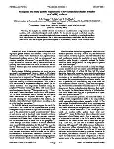
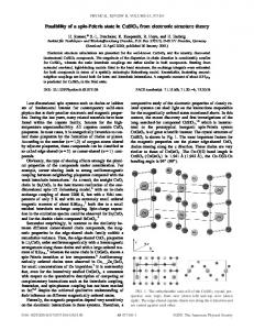
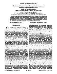
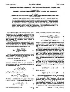
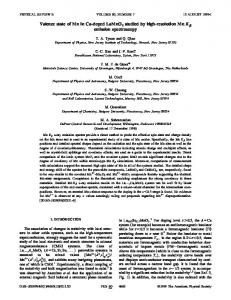
A simple experiment showed the crucial importance of the surrounding atmosphere on the electrical properties of the SWNTm. The ER variations of samples previously stored in air were studied during the first thermal outgassing cycle ( P⬍4⫻10⫺5 mbar). Figure 1 shows the electrical resistivity variation of a compacted SWNT mat during successive thermal cycles. In the step AB, the ‘‘as prepared’’ sample was maintained at 25 °C and pumped from the atmospheric pressure down to 10⫺5 mbar. Initially, the resistance increases while gas is removed from the sample. After 30 min the value of the resistance stabilizes 共point B兲. The total resistance increase is about 17%. A first heating from 25 °C to 220 °C 共step BC兲 during 1 h leads to a quasiexponential decrease of the resistance with an activation energy of about 13 meV. During the next 3 h 共step CD兲 the temperature was kept constant 共220 °C兲. Between D and E, the outgassed sample was cooled down to 25 °C still under vacuum. At this stage, the resistance versus temperature data fits to an Arrhenius law 10 000
©2000 The American Physical Society
PRB 62
BRIEF REPORTS
FIG. 1. Electrical resistance variations versus the temperature of the sample during the first thermal cycles. A resistance increase of 17% after room-temperature pumping is first observed 共A to B兲. But after a thermal cycle including 1-h ramp heating up to 220 °C 共B to C兲, pumping for 3 h at 220 °C 共C to D兲, and cooling down 共D to E兲, the final sample resistance was found noticeably higher 共E兲. Further thermal cycles exhibit superimposed traces 共E-F-G兲. This shows that high-temperature outgassing is necessary before achieving reproducible behavior.
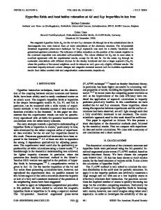
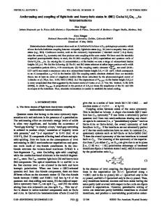
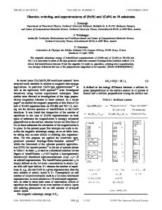
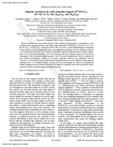
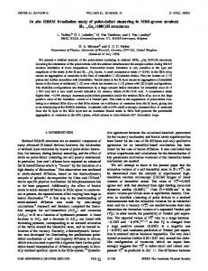
with an activation energy of about 20 meV. We observe that BC and DE traces are not identical. In fact, the roomtemperature resistance of the carefully outgassed sample 共E兲 is not only significantly higher than the ‘‘as prepared’’ one 共A兲 but is also noticeably higher than the ‘‘pumped only’’ sample 共B兲. Further cooling down 共step EF兲 or heating up 共FG兲 of the same outgassed sample exhibits perfectly superimposed traces. Starting from an outgassed sample, 50 l of distillated water were injected in the resistance measurement system 共volume of 1 l兲. All the experimental apparatus was maintained at 25 °C to establish an homogeneous pressure distribution inside. Figure 2 shows the evolution of the sample resistance during exposure to water vapor. During the first few minutes after injection a small resistance increase occurs, followed by a more important decrease with a time constant larger than 10 h. We notice that heating the exposed sample under vacuum at 220 °C led to total recovery of the resistance value in a few hours. These observations clearly show that water vapor is responsible for the variation of resistance in the exposed
FIG. 2. Sample resistance evolution after the injection of 50 l of distillated water. After a noticeable 共but relatively small兲 resistance increase, a more important decrease is clearly seen with a time constant larger than 10 h. Heating the exposed sample under vacuum at 220 °C led to recovery in a few hours.
10 001
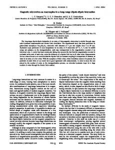
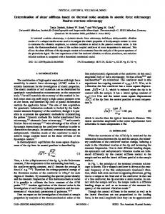
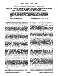
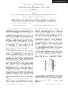
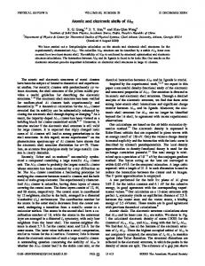
FIG. 3. Sample resistance evolution versus the water volume injected 共5-l H2O injection兲. The inset depicts the first three injections confirming the increase of the resistance in the beginning of the water exposure. The amplitude of the resistance variation is around 0.3% for the first two steps 共increasing resistance兲 but around 4% beyond the fourth injection 共decreasing resistance兲.
sample. Starting again from the same outgassed sample, we now inject water in 5-l steps. Figure 3 shows the sample resistance evolution versus the water volume injected. Every arrow corresponds to 5-l H2O injection. The inset depicts the first three injections confirming the increase of the resistance in the beginning of the water exposure (dR/dV⬎0) where V is the total injected liquid water volume. The amplitude of the resistance variation is around 0.3% for the first two steps and much higher 共4%兲 beyond the fourth one, after which the resistance versus the injected water volume becomes negative (dR/dV⬍0). Conductance variation of the sample versus injected water volume is displayed on Fig. 4. The i conductance value associated to i⫻5 l volume of injected water corresponds to the sample conductance just before the i⫹I injection. To explain the data we propose the following scenario. As it has been demonstrated by theoretical calculation and experimental observations,5,13 individual semiconducting SWNT or a mixture of metallic and semiconducting nanotubes show a global p-type semiconducting behavior. The electrical resistivity in such a system is dominated by holes scattering through the material. The Fermi level of single semiconducting SWNT is typically located at 25 mV above the valence band13. This energy value is in good agreement with the activation energy measured in our outgassed sample. Our previous work12 and many others recent works have established that SWNT electrical resistance exhibits an important sensitivity upon exposure to gaseous molecules such as CO2, NO2, NH3, or O2. 11,13,14 The effect of such an exposure strongly depends on the chemical nature of species used. It has been suggested that NH3 molecules are depleting the hole population, shifting the valence band of the nanotube away from the Fermi level thus reducing conductance;13 on the other hand, exposure to NO2 molecules is supposed to increase the hole carriers density and to enhance the sample conductance.13 As we have proposed,12 H2O molecules can be adsorbed on the nanotube and act like electron donors in a p-type semiconductor.17 In a first step, the minute quantity of injected water reduces the holes density in the SWNT. For an injected volume of V⬃12 l all the holes of semiconducting SWNT become compensated by the water doping and the
BRIEF REPORTS
10 002
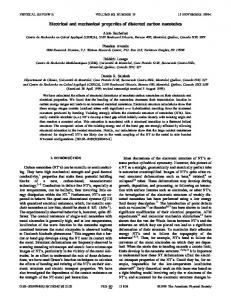
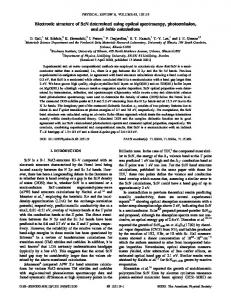
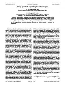
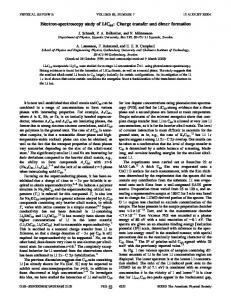
FIG. 4. Conductance of the sample versus injected water volume. The conductance values have been extracted from the Fig. 3 data. The i conductance value associated with i⫻5 l volume corresponds to the sample conductance just before the i⫹1 injection.
Fermi level shifts to the middle of the gap. After compensation, the SWNTm becomes an extrinsic n-type semiconductor. From the slopes of Fig. 4, we can estimate the ratio of electron to hole effective mass by 共 d⌬ /dV 兲 p/ 共 d⌬ /dV 兲 n⬃m n /m p ⫽0.12,
where ⌬ p ⬃(p 0 ⫺aV)/m p is the variation of the sample conductivity before the compensation, and ⌬ n ⬃(aV ⫺ p 0 )/m n is the variation of the sample conductivity after the compensation. p and n are, respectively, the electrical conductivity in the p-type and n-type regimes, aV is the number of electrons injected in the system 共supposed proportional to the water volume V, a is a positive constant兲, p 0 is the number of holes in the outgassed sample 共p 0 ⫽aV at compensation兲, and m n and m p are the electron and hole effective masses. Hall-effect measurements are in progress in order to confirm this result. In an attempt to analyze the observed time dependence in terms of a diffusion phenomenon, the variation of conductance (1/R⫺1/R 0 ) versus time is plotted in log-log scales 共Fig. 5兲 for the resistance decreasing part of Fig. 2 共time origin at the maximum resistance兲, R 0 being the initial resistance of the outgassed sample. In a normal diffusion process through isotropic material, the diffusion front is Gaussian and a log-log plot of the quantity of diffusing species versus the diffusion time led to a linear relationship with a 0.5 slope. In fact, the plot on Fig. 5 exhibits two separate quasilinear regimes: a very fast one, during the first 15 min, with a slope around 0.7, and a more slower one 共slope around 0.35兲 from 15 min to 14 h. If we suppose that the number of electrons injected in the SWNT mat is proportional to the injected volume of water 共below saturation兲, then the water diffusion in the SWNTm as shown on Fig. 5, is abnormal.
*Email:
[email protected] S. Iijima, Nature 共London兲 354, 56 共1991兲. 2 S. A. Tans et al., Nature 共London兲 386, 474 共1997兲. 3 C. T. White and T. N. Todorov, Nature 共London兲 393, 240 共1998兲. 4 R. Marte et al., Appl. Phys. Lett. 73, 2447 共1998兲. 1
PRB 62
FIG. 5. The variation of conductance (1/R⫺1/R 0 ) versus time is plotted in log-log scales, R 0 being the initial resistance of the outgassed sample. This plot exhibits two separate quasilinear regimes. First, a very fast regime with a slope around 0.7, and a more slower one 共slope around 0.3兲 until the end of the process.
The first part of the process is dominated by an enhanced diffusion 共0.7 slope兲. Enhanced diffusion is observed in porous layered systems, fractal geometry 共the diffusion front is more than two-dimensional兲, or more exotic systems.18 In our case, the compacted sample exhibits different porosity scales 共porosity between tubes inside the bundles, between the bundles, and between aggregates of bundles,...兲. A water molecule will then undergo a series of independent steps with a broad distribution in length while diffusing in the sample that might explain the observed effect. For a longer time scale, the propagation is dominated by a ‘‘subdiffusive’’ behavior 共slope 0.3兲. This abnormal diffusion is more frequent19 and can be well explained by a trapping mechanism associated with the adsorption of a water molecule outside and/or inside the bundles. CONCLUSION
To summarize, our experiments have shown that the electronic properties of SWNT can be deeply modified by the presence, in the surrounding atmosphere or inside poorly degassed SWNTm, of minute quantities of H2O. In particular, the conductivity type of the SWNT can be changed from p-type to n-type by adsorption of H2O water acting as an electron donor. An important consequence of this study is that careful preparation of SWNT should include hightemperature degassing, and that only dry, high purity gases should be used in order to avoid artifacts when studying their effects on nanotubes. ACKNOWLEDGMENTS
We are grateful to the Dr. P. Bernier’s group for providing the electric-discharge-produced SWNT samples 共L. Vaccarini, S. Tahir, and R. Aznar兲. We thank E. Alibert for efficient technical support, and Dr. F. Molino and Dr. J. L. Bantignies for helpful discussions. S. J. Tans, R. M. Verschueren, and C. Dekker, Nature 共London兲 393, 49 共1998兲. 6 S. Paulson et al., Appl. Phys. Lett. 75, 2936 共1999兲. 7 A. Bezryadin et al., Phys. Rev. Lett. 80, 4036 共1998兲. 8 R. Gaa´l, J.-P. Salvetat, and L. Forro´, Phys. Rev. B 61, 7320 共2000兲. 5
PRB 62
BRIEF REPORTS
L. Grigorian et al., Phys. Rev. B 58, R4195 共1998兲. C. Bower, S. Suzuki, and K. Tanigaki, Appl. Phys. A: Mater. Sci. Process. 67, 47 共1998兲. 11 P. G. Collins, M. Ishigami, and A. Zettl, Bull. Am. Phys. Soc. 44, 1889 共1999兲. 12 C. Marlie`re et al., in Proceeding of the Material Research Society, Boston, 1999 共Materials Research Society, Pittsburg, in press兲. 13 J. Kong et al., Science 287, 622 共2000兲.
10 003
P. G. Collins et al., Science 287, 1801 共2000兲. C. Journet and P. Bernier, Appl. Phys. A: Mater. Sci. Process. 67, 1 共1998兲. 16 L. Vaccarini et al., Synth. Met. 103, 2492 共1999兲. 17 H. Aria and T. Seiyama, Sensor: A Comprehensive Survey 共VCH Verlag, Weinheim, 1992兲, Vol. 3, p. 371. 18 J. P. Bouchaud et al., Phys. Rev. Lett. 64, 2503 共1990兲. 19 J. P. Bouchaud et al., J. Phys. II 1, 1465 共1991兲.
9
14
10
15