Value Function Approximation in Reinforcement Learning using the ...

Value Function Approximation in Reinforcement Learning using the Fourier Basis George Konidaris

Sarah Osentoski

Technical Report UM-CS-2008-19 Autonomous Learning Laboratory Computer Science Department University of Massachusetts Amherst {gdk, sosentos}@cs.umass.edu Abstract We describe the Fourier Basis, a linear value function approximation scheme based on the Fourier Series. We empirically evaluate its properties, and demonstrate that it performs well compared to Radial Basis Functions and the Polynomial Basis, the two most popular fixed bases for linear value function approximation, and is competitive with learned Proto-Value Functions even though no extra experience or computation is required.

1

Introduction

Reinforcement learning in continuous state spaces requires function approximation. Most work in this area focuses on linear function approximation, where the value function is represented as a weighted linear sum of a set of features (also known as basis functions) computed from the available state variables. Linear function approximation results in a simple update rule and quadratic error surface, even though the basis functions themselves may be arbitrarily complex. Reinforcement learning researchers have employed a wide variety of basis function schemes, most commonly Radial Basis Functions (RBFs) and CMACs (Sutton and Barto, 1998). For most problems, choosing the right basis function set is criticial for successful learning. Unfortunately, most approaches require significant design effort or problem insight, and no basis function set is both sufficiently simple and sufficiently reliable to be generally satisfactory. Recent work (Mahadevan, 2005) has focused on learning basis function sets from experience, removing the need to design a function approximator but introducing the need to gather data to create one before learning can take place. In the applied sciences the most common continuous function approximation method is the Fourier Series. Although the Fourier Series is a simple and effective function approximator with solid theoretical underpinnings, it is almost never used for value function approximation. In this paper we describe the Fourier Basis, a linear function approximation scheme that uses the terms of the Fourier Series as basis functions, resulting in a simple fixed basis scheme that should perform well generally. We present results that show that it performs well compared to Radial Basis Functions and the Polynomial Basis, the fixed bases most commonly used for linear value function approximation, and is competitive with learned Proto-Value Functions even though no extra experience or computation is required.

1

2

Background

A continuous-state Markov Decision Process (MDP) can be described as a tuple: a a M = hS, A, Pss 0 , Rss0 i, a where S ⊂ Rd is a set of possible state vectors, A is a discrete set of actions, Pss 0 is the transition model (modelling a the probability of moving from one state to another given an action), and Rss0 is the reward function.

The goal of reinforcement learning is to learn a policy π that maps a state vector to an action so as to maximize return a (discounted sum of rewards). When Pss 0 is known, this can be achieved by learning a value function V that maps a a given state vector to return, and selecting actions that result in the states with highest V . When Pss 0 not available, the agent must learn an action-value function Q that maps state-action pairs to expected return. Since the theory underlying the two cases is similar in the discussions that follow we consider only the value function case. V is commonly approximated as a weighted sum of a set of given basis functions φ1 , ..., φn : V¯ (x) =

n X

wi φi (x).

(1)

i=1

This is termed linear value function approximation since learning then entails finding the set of weights w = [w1 , ..., wn ] corresponding to an approximate optimal value function V¯ ∗ , and the value function is linear in w. Linear function approximation methods are attractive because they result in simple update rules (often using gradient descent) and possess a quadratic error surface that (except in degenerate cases) has a single minimum. In addition, they can potentially represent very complex value functions since the basis functions themselves can be arbitrarily complex.

2.1

The Polynomial Basis

Given a set of n state variables x = [x1 , ..., xn ], the simplest linear scheme is to use each variable directly as a basis function along with a single constant basis function, and set φ0 (x) = 1 and φi (x) = xi . However, most interesting value functions are too complex to be represented this way. This scheme was therefore generalized to the Polynomial Basis (Lagoudakis and Parr, 2003): φi (x) =

n Y

m

xj j ,

(2)

j=1

where each mj is an integer between 0 and k. We describe such a basis as an order k Polynomial Basis.

2.2

Radial Basis Functions

Another common basis scheme is Radial Basis Functions: φi (x) = √

1

2

2πσ 2

e−||ci −x||

/2σ 2

,

(3)

for a given set of centers ci and variance σ 2 . The centers are typically distributed evenly along each dimension, leading 2 to k n centers for a given k. The parameter σ 2 can be varied but is often set to k−1 . One advantage of RBFs is that they only generalize locally—changes in one area of the state space do not affect the entire state space. However, this limited generalization is often reflected in slow initial performance.

2

2.3

Proto-Value Functions

Recent research has focused on learning basis functions given experience. The most prominent type of learned basis functions are Proto-Value Functions or PVFs (Mahadevan, 2005). In their simplest form, an agent builds an adjacency matrix A by experience and then computes the Laplacian L of A: L = (D − A),

(4)

where D is a diagonal matrix with D(i, i) being the out-degree of state i. The eigenvectors of L form a set of bases that respect the topology of the state space (as reflected in A), and can be used as a set of orthogonal bases for a discrete domain. Mahadevan et al. (2006) extended PVFs to continuous domains, where a local distance metric is required to construct the graph and an out-of-sample method (which may be expensive to compute) is required for obtaining the values of each basis function at states not represented in A. Although the given results are promising, PVFs in continuous spaces require not only a large set of samples to produce the adjacency matrix and an expensive eigenvector decomposition to build the basis functions, but also require the programmer to make several potentially difficult design decisions.

3

The Fourier Basis

In this section we describe the Fourier Series for one and multiple variables, and use it to define the univariate and multivariate Fourier Bases.

3.1

The Univariate Fourier Series

The nth degree Fourier expansion of function f (x) with period T is given by:  n  2π 2π a0 X ak cos(k x) + bk sin(k x) , + f¯(x) = 2 T T

(5)

k=1

where ak = bk =

2 T

Z

2 T

Z

T

2π x) dx T

(6)

2π x) dx. T

(7)

f (x) cos(k 0 T

f (x) sin(k 0

For the remainder of this paper we assume for simplicity that T = 2, with the variables of the function we wish to approximate scaled appropriately. In the reinforcement learning setting f is unknown and so we cannot compute a0 , ..., an and b1 , ..., bn , but we can consider them coefficients to be learned in a linear function approximation scheme, setting:  i=0  1 cos( i+1 πx) i > 0, i odd φi (x) = 2  sin( 2i πx) i > 0, i even. Thus a full nth order Fourier approximation to a one-dimensional value function results in a linear function approximator with 2n + 1 terms. However, as we shall see below, we can usually use only n + 1 terms.

3

3.2

Even, Odd and Non-periodic Functions

If f is known to be even (that is, f (x) = f (−x), so that f is symmetric about the y-axis), then ∀i > 0, ai = 0 and we do not need to include the sin terms. This results in a value function that is guaranteed to be even, and reduces the number of terms required for an nth order Fourier approximation to n + 1. Similarly, if f is known to be odd (that is, f (x) = −f (−x), so that f is symmetric with respect to the origin) then ∀i > 0, bi = 0 and we can omit the cos terms. However, in general value functions are not even, odd, or periodic (or at least not known to be in advance). In such cases, we can define our approximation over [−1, 1] but only project the relevant variable to [0, 1]. This results in a function that is periodic on [−1, 1] but unconstrained on (0, 1]. Moreover, we are now free to choose whether or not the function is even or odd over [−1, 1] so that we can drop half of the terms in the approximation. In general, we expect that it will be better to use the “half-odd” approximation and drop the sin terms because it results in only a slight discontinuity at the origin. Thus, we define the univariate kth order Fourier Basis as: φi (x) = cos(iπx),

(8)

for i = 0, ..., k.

3.3

The Multivariate Fourier Series

The Fourier expansion of the multivariate function F (x) with period T in m dimensions is:  X 2π 2π F¯ (x) = ac cos( c.x) + bc sin( c.x) , T T c

(9)

where c = [c1 , ..., cm ], ci ∈ [0, ..., n], 0 ≤ i ≤ m. This results in 2(n + 1)m basis functions for an nth order full Fourier approximation to a value function in m dimensions, which can be reduced to (n + 1)m if we drop either the sin or cos terms for each variable as described above. We thus define the kth order Fourier Basis for m variables: φi (x) = cos(πci · x),

(10)

where ci = [c1 , ..., cm ], cj ∈ [0, ..., k], 0 ≤ j ≤ m. Each basis function thus has a coefficient vector c that attaches an integer coefficient (less than or equal to k) to each variable in x; the basis set is obtained by systematically varying the variables in c. This basis has the benefit of being easy to compute accurately even for high degrees, since cos is bounded in [−1, 1], and its arguments are formed by multiplication and summation rather than exponentiation. Although the Fourier Basis seems like a natural choice for value function approximation, we know of very few instances (e.g., Kolter and Ng (2007)) of its use in reinforcement learning, and no empirical study of its properties.

3.4

Variable Coupling

When applying reinforcement learning to continuous domains it is common to use an approximation scheme that assumes that each variable contributes independently to the value function. For example, an order 1 Polynomial Basis function contains φ terms for 1, x1 , x2 and x1 x2 ; assuming that x1 and x2 contribute independently means that we can drop the x1 x2 term. We call such a basis uncoupled. For higher order function approximators, uncoupling removes the curse of dimensionality: for an order k Polynomial Basis with 4 variables, the full basis has (k+1)4 terms, whereas the uncoupled basis has only 4(k+1) terms. Although this can lead to bad approximations (because in many cases the variables do not contribute independently) in many continuous domains it does not significantly degrade performance. However, a more sophisticated approach would involve the use of prior knowledge about which variables are likely to interact to obtain a smaller but still accurate function approximator. 4

The Fourier Basis facilitates this through constraints of c, the coefficient vector used in equation 10. For example, we can obtain an uncoupled basis by requiring that only one element of c is ever non-zero. Alternatively, if we know that the interaction of variables xi and xj is important for learning then we can constrain c so that only ci and cj can be non-zero simultaneously. We expect that most domains in which a decoupled basis performs badly are actually weakly coupled, in that we can use very low-order terms for the interaction between variables and high-order order terms for each variable independently. The Fourier Basis lends itself naturally to implementing such a scheme.

4 4.1

Empirical Evaluation The Swing-Up Acrobot

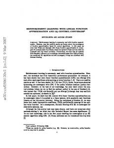
The acrobot is an underactuated two-link robot, show in Figure 1, where the first link is suspended from a point and the second is able to exert torque. The goal of the swing-up acrobot task is to swing the tip of the acrobot’s second joint one unit above the level of its suspension, much like a gymnast hanging from a pole and swinging above it using their waist. Since the acrobot is underactuated it cannot do this directly; instead it must swing back and forth to gain momentum. The resulting task has four continuous variables (an angle and a velocity for each joint) and three possible actions (exerting a negative, positive or zero unit of torque on the middle joint). Sutton and Barto (1998) contains a more detailed description.

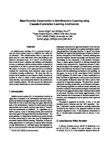
Figure 1: The Acrobot. We employed Sarsa(λ) (γ = 1.0, λ = 0.9,  = 0) with Fourier Bases of orders 3 (resulting in 256 basis functions), 5 (resulting in 1296 basis functions) and 7 (resulting in 4096 basis functions) and RBF, Polynomial and PVF bases of equivalent sizes to empirically compare their performance on the Acrobot task. (We did not run PVFs with 4096 basis functions because the nearest-neighbour calculations for a graph that size proved too expensive) We systematically varied α (the gradient descent term) to obtain the best performance for each basis function type and order combination. The resulting α values are shown in Table 1. The PVFs were built using the Normalized Laplacian: L = D−1/2 (D − W )D−1/2 , scaling the resulting eigenvectors so that they were in the range [−1, 1]. We also rescaled by Acrobot state variables by [1, 1, 0.05, 0.03] for local distance calculations. We found that a random walk did not suffice to collect samples that adequately cover the state space, and thus biased the sample collection to only keep examples where the random walk actually reached the target within 800 steps. We kept 50 of these episodes, leading to a sample size of approximately 3200 samples. We subsampled these initial samples to graphs of 1200 or 1400 points, created using nearest 30 neighbors. We did not optimize these settings as well as might have been possible, and thus the PVF averages are not as good as they could have been. However, our intention was to consider the performance of each method as generally used, and a full exploration of the parameters of PVF methods (or better construction methods, e.g. Johns et al. (2007); Mahadevan and Maggioni (2007)) was beyond the scope of this work. We ran 20 episodes averaged over 100 runs for each type of learner. The results, shown in Figure 2, demonstrate that the Fourier Basis learners outperformed all other types of learning agents for all sizes of function approximators. 5

Basis Fourier RBF Poly PVF

O(3) 0.001 0.0075 0.0075 0.0075

O(5) 0.0005 0.001 0.0075 0.0075

O(7) 0.0001 0.00075 0.01 —

Table 1: α values used for the Swing-Up Acrobot. In particular, the Fourier Basis performs better initially than the Polynomial Basis (which generalizes broadly) and converges to a better policy than the RBF Basis (which generalizes locally). It also performs slightly better than PVFs, even though the Fourier Basis is a fixed, rather than learned, basis. 1400 O(5) Fourier 1200

6 RBFs

1200

1000

1000

900

1296 PVFs 1000

800 700

Steps

800

600 Steps

800 Steps

O(7) Fourier 8 RBFs O(7) Polynomial

O(5) Polynomial O(3) Fourier 4 RBFs O(3) Polynomial 256 PVFs

600 600

500 400

400

400

300 200

200

200

100

0

0 0

2

4

6

8

10 12 Episodes

14

16

18

20

0

5

10 Episodes

(a)

(b)

15

20

0

0

2

4

6

8

10 12 Episodes

14

16

(c)

Figure 2: Learning curves for agents using (a) order 3 (b) order 5 and (c) order 7 Fourier Bases, and RBFs and PVFs with corresponding number of basis functions. However, the value function for Acrobot does not contain any discontinuities, and is therefore not the type of problem that PVFs are designed to solve. In the next section, we consider a continuous domain with an obstacle that induces a discontinuity in the value function.

4.2

The Discontinuous Room

In the Discontinuous Room, show in Figure 3, an agent in a room must reach a target; however the direct path to the target is blocked by a wall, which the agent must go around. The room measures 10x6 units, and the agent has four actions which move it 0.5 units in each direction. This domain is intended as a simple continuous domain with a large discontinuity, to empirically determine how the Fourier Basis handles such a discontinuity compared to Proto Value Functions, which were specifically designed to handle discontinuities by modelling the connectivity of the state space. In order to make a reliable comparison, agents using PVFs were given a perfect adjacency matrix containing every legal state and transition, thus avoiding sampling issues and removing the need for an out-of-sample extension method. Figure 4 shows learning curves for agents in the Discontinuous Room learning using Sarsa(λ) (γ = 0.9, λ = 0.9,  = 0) using Fourier Bases of order 5 (α = 0.025) and order 7 (α = 0.025) and agents using 36 (α = 0.025) and 64 (α = 0.025) PVFs. The agents using the Fourier Basis do not initially perform as well as the agents using PVFs, probably because of the discontinuity, but this effect is transient and the Fourier Basis agents eventually perform better.

6

18

20

Figure 3: The Discontinuous Room, where an agent must move from the lower left corner to the upper left corner by skirting around a wall through the middle of the room. 1000 800 600

Reward

400 200 0 −200 36 PVFs −400

64 PVFs O(5) Fourier

−600 −800

O(7) Fourier 0

10

20

30

40

50 60 Episodes

70

80

90

100

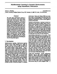
Figure 4: Learning curves for the Discontinuous Room, for agents using O(5) and O(7) Fourier Bases and agents using 36 and 64 PVFs. Figure 5 shows example value functions for for an agent using an order 7 Fourier Basis and a corresponding agent using 64 PVFs. The PVF value function is clearly a better approximation to an optimal policy value function, and in particular shows very precise modelling of the discontinuity around the wall. In contrast, the Fourier Basis value function is noisier and does not model the discontinuity as cleanly. However, the results in Figure 4 suggest that this does not significantly impact the quality of the resulting policy, and it appears that the Fourier Basis agent has learned to avoid the discontinuity. This suggests that, at least for continuous problems with a small number of discontinuities, the Fourier Basis is sufficient, and that the extra complexity (in terms of samples and computation) of PVFs only becomes really necessary in more complex problems.

4.3

Mountain Car

The Mountain Car (Sutton and Barto, 1998), as shown in Figure 6 is an underpowered car that must drive up a steep cliff in a valley; to do so, it must first accelerate up the back of the valley, and then use the resulting momentum to drive up the other side. This induces a steep discontinuity in the value function which makes learning difficult, which we use to examine the properties of the Fourier Basis in a domain very difficult for bases with global support. We employed Sarsa(λ) (γ = 1.0, λ = 0.9,  = 0) with Fourier Bases of orders 3 and 5, and RBFs and PVFs of equivalent sizes (we were unable to learn with the Polynomial Basis). Here we found it best to scale the α values for 1 the Fourier Basis by 1+m , where m was the maximum degree of the basis function. This allocated lower learning 7

(a)

(b)

Figure 5: Value functions for the Discontinuous Room from agents using (a) an O(7) Fourier Basis and (b) 64 PVFs.

Figure 6: The Mountain Car. rates to higher frequency basis functions. The α values used for learning are shown in Table 2. Basis Fourier RBF PVF

O(3) 0.025 0.025 0.01

O(5) 0.025 0.025 0.025

Table 2: α values used for Mountain Car. The results (shown in Figure 7) indicate that for low orders, the Fourer Basis outperforms RBFs and PVFs. For higher orders, we see a repetition of the learning curve in Figure 4, where the Fourier Basis initially performs worse (because it does not model the discontinuity in the value function well) but converges to a better solution. Thus, although the Fourier Basis is not always the best choice for domains with discontinuities, it works reliably.

5

Discussion

Our results show that the Fourier Basis provides a simple and reliable basis for value function approximation. We expect that for many problems, the Fourier Basis will be sufficient to learn a good value function without any extra work. If necessary, the ability to include prior knowledge about symmetry or variable interaction provides a simple and useful tool to induce structure in the value function.

8

1100

1400 O(3) Fourier 4 RBFs 16 PVFs

1200

6 RBFs O(5) Fourier 36 PVFs

1000 900 800

1000

700 Steps

Steps

800

600

600 500 400

400

300 200

200 0

0

5

10 Episodes

15

100

20

(a)

0

5

10 Episodes

15

20

(b)

Figure 7: Learning curves for agents using (a) order 3 (b) order 5 Fourier Bases, and RBFs and PVFs with corresponding number of basis functions. The one area in which we find that the Fourier Basis has difficulty representing is flat areas in value functions; moreover, for high order Fourier Basis approximations sudden discontinuities may induces “ringing” around the point of discontinuity, known as Gibbs phenomenon (Gibbs, 1898). This may result in policy difficulties near the discontinuity. Another challenge posed by the Fourier Basis (and all fixed basis function approximators) is how to select basis functions when a full order approximation of reasonable size is too large to be useful. PVFs, by contrast, scale with the size of the sample graph (and thus could potentially take advantage of the underlying complexity of the manifold). It may be possible to do something similar by sampling and then using the properties of the resulting data to select a good set of Fourier Basis functions for learning. Another potential difficulty we have encountered is that the use of a single α term in gradient-descent based algorithms (such as Sarsa(λ)) creates difficulties for very high-order Fourier Basis function approximators. This is because a single α must be found that is able to handle basis functions of very different frequencies. This difficulty will affect PVFs and the Polynomial Basis, but not Radial Basis functions because each RBF is the same size. Least-squares based methods are not affected by this problem. Nevertheless, our experiences with the Fourier Basis show that this simple and easy to use basis set reliably performs well on a range of different problems. As such, although it may not perform well for domains with several significant discontinuities, its simplicity and reliability suggest that the Fourier Basis should be the first function approximator used when reinforcement is applied to a problem.

6

Summary

We have described the Fourier Basis, a linear function approximation scheme using the terms of a Fourier series as features. Our experimental results show that this simple and easy to use basis performs well compared to two popular fixed bases and a learned set of basis functions in two continuous reinforcement learning benchmarks, and is competitive with a popular learned basis even though no extra experience or computation is required.

9

References Gibbs, J. (1898). Fourier series. Nature, 59(200). Johns, J., Mahadevan, S., and Wang, C. (2007). Compact spectral bases for value function approximation using kronecker factorization. In Proceedings of the Twenty-second National Conference on Artificial Intelligence (AAAI07). Kolter, J. and Ng, A. (2007). Learning omnidirectional path following using dimensionality reduction. In Proceedings of Robotics: Science and Systems. Lagoudakis, M. and Parr, R. (2003). Least-squares policy iteration. Journal of Machine Learning Research, 4, 1107– 1149. Mahadevan, S. (2005). Proto-value functions: Developmental reinforcement learning. In Proceedings of the Twenty Second International Conference on Machine Learning. Mahadevan, S. and Maggioni, M. (2007). Proto-value functions: A laplacian framework for learning representation and control in markov decision processes. Journal of Machine Learning Research, 8, 2169–2231. Mahadevan, S., Maggioni, M., Ferguson, K., and Osentoski, S. (2006). Learning representation and control in continuous markov decision processes. In Proceedings of the Twenty First National Conference on Artificial Intelligence. Sutton, R. and Barto, A. (1998). Reinforcement Learning: An Introduction. MIT Press, Cambridge, MA.

10