Vision-based Mobile Robot Localization And Mapping ... - CiteSeerX

Vision-based Mobile Robot Localization And Mapping using Scale-Invariant Features Stephen Se, David Lowe, Jim Little Department of Computer Science University of British Columbia Vancouver, B.C. V6T 1Z4, Canada {se,lowe,little}@cs.ubc.ca Abstract A key component of a mobile robot system is the ability to localize itself accurately and build a map of the environment simultaneously. In this paper, a vision-based mobile robot localization and mapping algorithm is described which uses scale-invariant image features as landmarks in unmodified dynamic environments. These 3D landmarks are localized and robot ego-motion is estimated by matching them, taking into account the feature viewpoint variation. With our Triclops stereo vision system, experiments show that these features are robustly matched between views, 3D landmarks are tracked, robot pose is estimated and a 3D map is built.

1

Introduction

Mobile robot localization and mapping, the process of simultaneously tracking the position of a mobile robot relative to its environment and building a map of the environment, has been a central research topic for the past few years. Accurate localization is a prerequisite for building a good map, and having an accurate map is essential for good localization. Therefore, Simultaneous Localization And Map Building (SLAMB) is a critical underlying factor for successful mobile robot navigation in a large environment, irrespective of the higher-level goals or applications. To achieve SLAMB, there are different types of sensor modalities such as sonar, laser range finders and vision. Many early successful approaches [2] utilize artificial landmarks, such as bar-code reflectors, ultrasonic beacons, visual patterns, etc., and therefore do not function properly in beacon-free environments. Vision-based approaches using stable natural landmarks in unmodified environments are highly desirable for a wide range of applications. Harris’s 3D vision system DROID [8] uses the visual motion of image corner features for 3D reconstruction. Kalman filters are used for tracking features

from which it determines both the camera motion and the 3D positions of the features. It is accurate in the short to medium term, but long-term drifts can occur. The ego-motion and the perceived 3D structure can be self-consistently in error. It is an incremental algorithm and it runs at near real-time. A stereo vision algorithm for mobile robot mapping and navigation is proposed in [13], where a 2D occupancy grid map is built from the stereo data. However, since the robot does not localize itself using the map, odometry error is not corrected and hence the map may drift over time. [10] proposed combining this 2D occupancy map with sparse 3D landmarks for robot localization, and corners on planar objects are used as stable landmarks. However, landmarks are used for matching only in the next frame but not kept for matching subsequent frames. Markov localization was employed by various teams with success [15, 17]. For example, the Deutsches Museum Bonn tour-guide robot RHINO [3, 6] utilizes a metric version of this approach with laser sensors. However, it needs to be supplied with a manually derived map, and cannot learn maps from scratch. Thrun et al. [19] proposed a probabilistic approach for map building using the Expectation-Maximization (EM) algorithm. The E-step estimates robot locations at various points based on the currently best available map and the M-step estimates a maximum likelihood map based on the locations computed in the E-step. It searches for the most likely map by simultaneously considering the locations of all past sonar scans. After traversing a cyclic environment, the algorithm revises estimates backward in time. It is a batch algorithm and cannot be run in real-time. Unlike RHINO, the latest museum tour-guide robot MINERVA [18] learns its map and uses camera mosaics of the ceiling for localization in addition to the laser scan occupancy map. It uses the EM algorithm in [19]

to learn the occupancy map and the novelty filter in [6] for localization. The Monte Carlo Localization method was proposed in [5] based on the CONDENSATION algorithm [9]. This vision-based Bayesian filtering method uses a sampling-based density representation. Unlike the Kalman filter based approaches, it can represent multi-modal probability distributions. Given a visual map of the ceiling obtained by mosaicing, it localizes the robot using a scalar brightness measurement. Sim and Dudek [16] proposed learning natural visual features for pose estimation. Landmark matching is achieved using principal components analysis and a tracked landmark is a set of image thumbnails detected in the learning phase, for each grid position in pose space. Using global registration and correlation techniques, [7] proposed a method to reconstruct consistent global maps from laser range data reliably. Recently, Thrun et al. [20] proposed a novel realtime algorithm combining the strengths of EM algorithms and incremental algorithms. Their approach computes the full posterior over robot poses to determine the most likely pose, instead of just using the most recent laser scan as in incremental mapping. When closing cycles, backwards correction can be computed from the difference between the incremental guess and the full posterior guess. Most existing mobile robot localization and mapping algorithms are based on laser or sonar sensors, as vision is more processor intensive and stable visual features are more difficult to extract. In this paper, we propose a vision-based SLAMB algorithm by tracking SIFT features. As our robot is equipped with Triclops [14], a trinocular stereo system, the estimated 3D position of the landmarks can be obtained and hence a 3D map can be built and the robot can be localized simultaneously. The 3D map, represented as a SIFT landmark database, is incrementally updated over time and adaptive to dynamic environments. Section 2 explains the SIFT features and the stereo matching process. Ego-motion estimation by matching features across frames is described in Section 3 and SIFT database landmark tracking is presented in Section 4. Experimental results are shown in Section 5, where our 10m by 10m lab environment is mapped with more than 3000 SIFT landmarks. Section 6 describes some enhancements to the SIFT database. Finally, we conclude and discuss some future work in Section 7.

2

SIFT Stereo

SIFT (Scale Invariant Feature Transform) was developed by Lowe [12] for image feature generation in

(a)

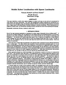
(b) (c) Figure 1: SIFT features found, with scale and orientation indicated by the size and orientation of the squares. (a) Top image. (b) Left image. (c) Right image. object recognition applications. The features are invariant to image translation, scaling, rotation, and partially invariant to illumination changes and affine or 3D projection. These characteristics make them suitable landmarks for robust SLAMB, since when mobile robots are moving around in an environment, landmarks are observed over time, but from different angles, distances or under different illumination. At each frame, we extract SIFT features in each of the three images, and stereo match them among the images. Matched SIFT features are stable and will serve as landmarks for the environment.

2.1

Generating SIFT Features

Key locations are selected at maxima and minima of a difference of Gaussian function applied in scale space. They can be computed by building an image pyramid with resampling between each level. Furthermore, SIFT locates key points at regions and scales of high variation, making these locations particularly stable for characterizing the image. [12] demonstrated the stability of SIFT keys to image transformations. Figure 1 shows the SIFT features found on the top, left and right images. The resolution is 320x240 and 8 levels of scales are used. A subpixel image location,

scale and orientation are associated with each SIFT feature. The size of the square surrounding each feature in the images is proportional to the scale at which the feature is found, and the orientation of the squares corresponds to the orientation of the SIFT features. Image Top Left Right

2.2

Number of SIFT features found 193 166 189

Stereo Matching

The right camera in the Triclops serves as the reference camera, as the left camera is at 10cm right beside it and the top camera is at 10cm directly above it. In addition to the epipolar constraint and disparity constraint, we also employ the SIFT scale and orientation constraints for matching the right and left images. Subpixel horizontal disparity is obtained for each match. These resulting matches are then matched with the top image similarly, with an extra constraint for agreement between the horizontal and vertical disparities. If a feature has more than one match satisfying these criteria, it is ambiguous and discarded so that the resulting matches are more consistent and reliable. From the positions of the matches and knowing the camera intrinsic parameters, we can compute the 3D world coordinates (X, Y, Z) relative to the robot for each feature in this final set. They can subsequently serve as landmarks for map building and tracking. The disparity is taken as the average of the horizontal disparity and the vertical disparity. The orientation and scale of each matched SIFT feature are taken as the average of the orientation and scale among the corresponding SIFT feature in the left, right and top images.

2.3

Results

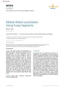
There are 106 matches between the right and left images shown in Figure 1. After matching with the top image, the final number of matches is 59. The result is shown in Figure 2(a), where each matched SIFT feature is marked; the length of the horizontal line indicates the horizontal disparity and the vertical line indicates the vertical disparity for each feature. Figures 2(b) and (c) show more SIFT stereo results for slightly different views when the robot makes some small motion. Figure Number of final matches Figure 2(a) 59 Figure 2(b) 66 Figure 2(c) 60 Relaxing some of the constraints above does not necessarily increase the number of final matches be-

(a)

(b) (c) Figure 2: Stereo matching results for slightly different views. Horizontal line indicates its horizontal disparity and vertical line indicates its vertical disparity. Line lengths are proportional to the corresponding disparities. Closer objects will have larger disparities. cause some SIFT features will then have multiple potential matches and therefore be discarded.

3

Ego-motion Estimation

We obtain [r, c, s, o, d, X, Y, Z] for each stereo matched SIFT feature, where (r, c) is the measured image coordinates in the reference camera, (s, o, d) are the scale, orientation and disparity associated with each feature, (X, Y, Z) are its 3D coordinates relative to the camera. To build a map, we need to know how the robot has moved between frames in order to put the landmarks together coherently. The robot odometry data can only give a rough estimate and it is prone to error such as drifting, slipping, etc. To find matches in the second view, the odometry allows us to predict the region to search for each match more efficiently. Once the SIFT features are matched, we can use the matches in a least-squares procedure to compute a more accurate camera ego-motion and hence better localization. This will also help adjust the 3D coordinates of the SIFT landmarks for map building.

3.1

Predicting Feature Characteristics

From the 3D coordinates of a SIFT landmark and the odometry data, we can compute the expected 3D relative position and hence the expected image coordinates and disparity in the new view. The expected scale is computed accordingly as it is inversely related to the distance. We can search for the appropriate SIFT feature match within a region (currently 5 by 5 pixels) in the next frame, using the disparity constraint together with the SIFT scale and orientation constraints.

3.2

Matching Results

For the images shown in Figure 2, the rough camera movement from the odometry is: Figure Figure 2(a) Figure 2(b) Figure 2(c)

(a)

Movement Initial position Forward 10cm Rotate clockwise 5◦

The frames are then matched: Figures to match Figure 2(a) and (b) Figure 2(b) and (c)

No. of matches 43 41

% of matches 73% 68%

Figure 3 shows the match results visually where the shift in image coordinates of each feature is marked. The white dot indicates the current position and the white cross indicates the new position; the line shows how each matched SIFT feature moves from one frame to the next, analogous to sparse optic flow. Figures 3(a) is for a forward motion of 10cm and Figures 3(b) is for a clockwise rotation of 5◦ . It can be seen that the matches found are very consistent.

3.3

Least-Squares Minimization

Once the matches are obtained, the ego-motion is determined by finding the camera movement that would bring each projected SIFT landmark into the best alignment with its matching observed feature. To minimize the errors between the projected image coordinates and the observed image coordinates, we employ a least-squares minimization [11] to compute this camera ego-motion. Although our robot can only move forward and rotate, we use a full 6 degrees of freedom for the general motion. Newton’s method computes a correction term to be subtracted from the initial estimate, using the error measurements between the expected projection of the SIFT landmarks and the image position observed for the matching feature. The Jacobian matrix is estimated numerically and Gaussian elimination with pivoting is employed to solve the linear system. The good feature matching quality implies very high percentage of inliers, and therefore, outliers are simply eliminated by discarding

(b) Figure 3: The SIFT feature matches between consecutive frames: (a) Between Figure 2(a) and (b) for a 10cm forward movement. (b) Between Figure 2(b) and (c) for a 5◦ clockwise rotation. features with significant residual errors E (currently 3 pixels). Minimization is repeated with the remainder matches to obtain the new correction term.

3.4

Results

We pass the SIFT feature matches in Figure 3 to the least-squares procedure with the odometry as the initial estimate of ego-motion. For between-frame movement over a smooth floor, odometry is quite accurate and can be used to judge the accuracy of the solution. The following results are obtained, where the least-squares estimate [X, Y, Z, θ, α, β] corresponds to the translations in X, Y, Z directions, yaw, pitch and roll respectively: Fig 3(a)

Odometry Z=10cm

3(b)

θ=5◦

Mean E 1.328 (pixels) 1.693 (pixels)

Least-Squares Estimate [1.353cm,-0.534cm,11.136cm, 0.059◦ ,−0.055◦ ,−0.029◦ ] [0.711cm,0.008cm,-0.9890cm, 4.706◦ ,0.059◦ ,−0.132◦ ]

4

Landmark Tracking

After matching SIFT features between frames, we would like to maintain a database containing the SIFT landmarks observed and use it to match features found in subsequent views. Each SIFT feature has been stereo matched and localized in 3D coordinates. Its entry in the database: [X, Y, Z, s, o, l] where (X, Y, Z) is the current 3D position of the SIFT landmark relative to the camera, (s, o) are its scale and orientation, and l is a count to indicate how many consecutive frames this landmark has been missed. Over subsequent frames, we would like to maintain this database, add new entries to it, track features and prune entries when appropriate, to cater for dynamic environments and occlusions.

4.1

Track Maintenance

Between frames, we obtain a rough estimate of camera ego-motion from robot odometry to predict the feature characteristics for each database landmark in the next frame. There are the following types of landmarks to consider: Type I. This landmark is not expected to be within view in the next frame. Therefore, it is not being matched and its miss count remains unchanged. Type II. This landmark is expected to be within view, but no matches can be found in the next frame. Its miss count is incremented by 1. Type III. This landmark is within view and a match is found according to the position, scale, orientation and disparity criteria described before. Its miss count is reset to 0. Type IV. This is a new landmark corresponding to a SIFT feature in the new view which does not match any existing landmarks in the database. All the Type III landmarks matched are then used in the least-squares minimization to obtain a better estimate for the camera ego-motion. The landmarks in the database are currently updated by averaging. This update can be replaced by some data fusion methods such as the Kalman filter [1] (Section 6.4). If there are insufficient Type III matches due to occlusion for instance, the odometry will be used as the ego-motion for the current frame.

4.2

Track Initiation

Initially the database is empty. When SIFT features from the first frame arrive, we start a new track for each of the features initializing their miss count l to 0. In subsequent frames, a new track is initiated for each of the Type IV landmarks.

4.3

Track Termination

If the miss count l of any landmark in the database reaches a predefined limit N (20 was used in experi-

ments), i.e., it has not been observed at its predicted position for N consecutive frames, this landmark track is terminated and pruned from the database. This removes features belonging to objects that moved in a dynamic environment.

4.4

Field of View

Firstly, we compute the expected 3D coordinates (X 0 , Y 0 , Z 0 ) from the current coordinates and the odometry. For a database landmark to be within the field of view in the next frame, we check Z 0 > 0 (not behind the camera), tan−1 (|X 0 |/Z 0 ) < 30◦ and tan−1 (|Y 0 |/Z 0 ) < 30◦ , as the Triclops camera lens field of view is around 60◦ wide.

4.5

Reference Coordinate Frame

We use the initial camera coordinate frame as the reference and make all the landmarks relative to this fixed frame. Therefore, Type I and Type II landmarks do not need to be transformed using the camera egomotion estimate at each frame. Matching the SIFT landmarks referenced to the initial frame with features observed in the current frame helps avoid error accumulation.

5

Experimental Results

SIFT feature detection, stereo matching, egomotion estimation and tracking algorithms have been implemented in our robot system. A SIFT database is kept to track the features over frames. As the robot camera Y location does not change much over flat ground, we reduce the estimation from 6 d.o.f. to 5, forcing the height change parameter to 0. Depending on the distribution of features in the scene, there is ambiguity between a yaw rotation and a sideways movement, which is a well-known problem. Moreover, we set a limit to the correction terms allowed for the least-squares minimization as the odometry for between-frame movement should be quite good. This will safeguard frames which have erroneous matches that may lead to excessive correction terms and mess up the subsequent estimation. As our ego-motion estimation determines the movement of the camera which is not placed in the centre of the robot, we need to adjust the odometry information to get the camera motion. The following experiment was carried out on the fly while the robot is moving around. We manually drive the robot to go around a chair in the lab for one loop and come back. At each frame, it keeps track of the SIFT landmarks in the database, adds new ones and updates existing ones if matched. Figure 4 shows some frames of the 320x240 image sequence (249 frames in total) captured while the robot is moving around. The white markers indicate

(a)

4 metres and then has come back with its trajectory shown in Figure 5. The maximum robot translation and rotation speeds are set to around 40cm/sec and 10◦ /sec respectively such that there are sufficiently many matches between consecutive frames. The accuracy of the ego-motion estimation depends on the SIFT landmarks and their distribution, the number of matches, etc. In this experiment, there are sufficiently many matches at each frame, ranging mostly between 40 and 60, depending on the particular part of the lab and the viewing direction. At the end when the robot comes back to the original position (0,0,0) judged visually: SIFT estimate: X:-2.09cm Y:0cm Z:-3.91cm θ:0.30◦ α:2.10◦ β:−2.02◦

(b)

(c) (d) Figure 4: Frames of an image sequence with SIFT features marked. (a) 1st frame. (b) 60th frame. (c) 120th frame. (d) 180th frame.

6

Our basic approach has been described above, but there are various enhancements dealing with the SIFT database that can help our tracking to be more robust and our map-building to be more stable.

6.1 1600

1400

1200

1000

800

600

400

200

0

−200

−400 −1000 −800

−600

−400

−200

0

200

400

600

800

1000

Figure 5: Bird’s eye view of the SIFT landmarks (including ceiling features) in the database after 249 frames. The cross at (0,0) indicates the initial robot position and the dashed line indicates the robot path. the SIFT features found. At the end, a total of 3590 SIFT landmarks, with 3D positions relative to the initial robot position, are gathered in the SIFT database. Figure 5 shows the bird’s eye view of these features. Consistent clusters are observed corresponding to chairs, shelves, posters, computers etc. in the scene. The robot has traversed forward more than

SIFT Database

Database Entry

In order to assess the reliability of a certain SIFT feature in the database, we need some information regarding how many times this feature has been matched and has not been matched so far. The new database entry is [X, Y, Z, s, o, m, n, l] where l is still the count for the number of times being missed consecutively, which is used to decide whether or not the feature should be pruned from tracking. m is a count for the number of times it has been missed so far and n is a count for the number of times it has been seen so far. Each feature has to appear at least 3 times (n ≥ 3) to be considered as a valid feature. This is to eliminate false alarms and noise, as it is highly unlikely that some noise will cause a feature to match in the right, left & top images for 3 times (a total of 9 camera views). In this experiment, we move the robot around the lab environment without the chair in the middle. In order to demonstrate visually that the SIFT database map is three-dimensional, we use a visualization package Geomview. Figure 6 shows several views of the 3D SIFT map from different angles in Geomview. We can see that the centre region is clear, as false alarms and noise features are discarded. Visual judgement indicates that the SIFT landmarks correspond well to actual objects in the lab.

6.2

Permanent Landmarks

In a scene where there could be many volatile features, e.g., when someone blocks the camera view for a while, stable features observed earlier are not matched for a number of consecutive frames, and will be discarded.

(a)

(b) (c) Figure 6: 3D SIFT database map viewed from different angles in Geomview. Each feature has appeared consistently in at least 9 camera views. (a) From top. (b) From left. (c) From right. Therefore, when the environment is clear, we can build a SIFT database beforehand and mark them as permanent landmarks, if they are valid (having appeared in at least 3 frames) and if the percentage of their occurrence, given by n/(n+m), is above a certain threshold. Afterwards, this set of reliable landmarks will not be wiped out even if they are being missed for many consecutive frames. They are important for subsequent localization after the view is unblocked.

6.3

Viewpoint Variation

Although SIFT features are invariant in image orientation and scale, they are image projections of 3D landmarks and hence vary with large changes of viewpoints and as different parts of the object are observed or part of the object is occluded. For example, when the front of an object is seen first, after the robot moves around and views the object from the back, the image feature is in general completely different. As the original feature may not be observable from this viewpoint, or observable but appear different, its miss count will increase gradually and it will be pruned even though it is still there. Therefore, we allow each SIFT landmark to have more than one SIFT characteristics, where each SIFT characteristic (scale and orientation) is associated with a view vector keeping track of the viewpoint from

which the feature is observed. Subsequently, if the new view direction differs from the original view direction by more than a threshold (currently set to 20◦ ), its miss count will not be incremented even if it does not match. This way we can avoid corrupting the feature information gathered earlier by the current partial view of the world. If a feature matches from a direction larger than the threshold, we add a new view vector with the associated SIFT characteristic to the existing landmark. Therefore, a database landmark can have multiple SIFT characteristics (si , oi , vi ) where si and oi are the scale and orientation for the view direction vi . Over time, if a landmark is observed from various directions, much richer SIFT information is gathered. The matching procedure is as follows: • compute view vector v between the database landmark and the current robot position • find the existing view direction vi associated with the database landmark which is closest to v, i.e., with minimal angle φ between the two vectors • check whether φ is less than 20◦ : – if so, update the existing s and o if feature matching succeeds, or increment miss count if feature matching fails – else, add a new entry of SIFT characteristics (s, o, v) to the existing landmark if feature matching succeeds The 3D positions of the landmarks are updated accordingly if matched.

6.4

Error Modeling

There are various errors such as noise and quantization associated with the images and the features found. They introduce inaccuracy in both the landmarks’ position as well as the least-squares estimation of the robot position. In stochastic mapping, a single filter is used to maintain estimates of landmark positions, the robot position and the covariances between them [4], with high computational complexity. In more recent work, we have employed a Kalman Filter [1] for each database SIFT landmark which now has a 3x3 covariance matrix for its position, assuming the independence of landmarks. When a match is found in the current frame, the covariance matrix in the current frame will be combined with the covariance matrix in the database so far, and its 3D position will be updated accordingly. An ellipsoidal uncertainty based on its covariance is associated with each landmark position. The ellipses shrink when the landmarks are matched over frames, indicating they are localized better. On the other hand, the ellipses expand when the landmarks are missed, indicating higher positional uncertainty.

7

Conclusion

In this paper, we proposed a vision-based SLAMB algorithm based on the SIFT features. Being scale and orientation invariant, SIFT features are good natural visual landmarks for tracking over long periods of time from different views. These tracked landmarks are used for concurrent robot pose estimation and 3D map building, with promising results shown. The algorithm currently runs at 2Hz for 320x240 images on our mobile robot with a Pentium III 700MHz processor. As the majority of the processing time is spent on SIFT feature extraction, MMX optimization is being investigated. At present, the map is re-used only if the robot starts up again at the last stop position or if the robot starts at the position of the initial reference frame. Preliminary work on the ‘kidnapped robot’ problem, i.e., initializing localization, has been positive. This will allow the robot to re-use the map at any arbitrary robot position by matching the rich SIFT database. We are currently looking into recognizing the return to a previously mapped area and detecting the occurrences of drift and to correct for it.

Acknowledgements

[8]

[9]

[10]

[11]

[12]

[13]

[14]

Our work has been supported by the Institute for Robotics and Intelligent System (IRIS III), a Canadian Network of Centres of Excellence.

References [1] Y. Bar-Shalom and T.E. Fortmann. Tracking and Data Association. Academic Press, Boston, 1988. [2] J. Borenstein, B. Everett, and L. Feng. Navigating Mobile Robots: Systems and Techniques. A. K. Peters, Ltd, Wellesley, MA, 1996. [3] W. Burgard, A.B. Cremers, D. Fox, D. Hahnel, G. Lakemeyer, D. Schulz, W. Steiner, and S. Thrun. The interactive museum tour-guide robot. In Proceedings of the Fifteenth National Conference on Artificial Intelligence (AAAI), Madison, Wisconsin, July 1998. [4] A.J. Davison and D.W. Murray. Mobile robot localisation using active vision. In Proceedings of Fifth European Conference on Computer Vision (ECCV’98) Volume II, pages 809–825, Freiburg, Germany, June 1998. [5] F. Dellaert, W. Burgard, D. Fox, and S. Thrun. Using the condensation algorithm for robust, vision-based mobile robot localization. In Proceedings of IEEE Conference on Computer Vision and Pattern Recognition (CVPR’99), Fort Collins, CO, June 1999. [6] D. Fox, W. Burgard, S. Thrun, and A.B. Cremers. Position estimation for mobile robots in dynamic environments. In Proceedings of the Fifteenth National Conference on Artificial Intelligence (AAAI), Madison, Wisconsin, July 1998. [7] J. Gutmann and K. Konolige. Incremental mapping of large cyclic environments. In Proceedings of the

[15]

[16]

[17]

[18]

[19]

[20]

IEEE International Symposium on Computational Intelligence in Robotics and Automation (CIRA), California, November 1999. C. Harris. Geometry from visual motion. In A. Blake and A. Yuille, editors, Active Vision, pages 264–284. MIT Press, 1992. M. Isard and A. Blake. Condensation - conditional density propagation for visual tracking. International Journal of Computer Vision, 29(1):5–28, 1998. J.J. Little, J. Lu, and D.R. Murray. Selecting stable image features for robot localization using stereo. In Proceedings of IEEE/RSJ International Conference on Intelligent Robotic Systems (IROS’98), Victoria, B.C., Canada, October 1998. D.G. Lowe. Fitting parameterized three-dimensional models to images. IEEE Trans. Pattern Analysis Mach. Intell. (PAMI), 13(5):441–450, May 1991. D.G. Lowe. Object recognition from local scaleinvariant features. In Proceedings of the Seventh International Conference on Computer Vision (ICCV’99), pages 1150–1157, Kerkyra, Greece, September 1999. D. Murray and C. Jennings. Stereo vision based mapping and navigation for mobile robots. In Proceedings of the IEEE International Conference on Robotics and Automation (ICRA’97), pages 1694–1699, New Mexico, April 1998. D. Murray and J. Little. Using real-time stereo vision for mobile robot navigation. In Proceedings of the IEEE Workshop on Perception for Mobile Agents, Santa Barbara, CA, June 1998. I. Nourbakhsh, R. Powers, and S. Birchfield. Dervish: An office-navigating robot. AI Magazine, 16:53–60, 1995. R. Sim and G. Dudek. Learning and evaluating visual features for pose estimation. In Proceedings of the Seventh International Conference on Computer Vision (ICCV’99), Kerkyra, Greece, September 1999. R. Simmons and S. Koenig. Probabilistic robot navigation in partially observable environments. In Proceedings of the Fourteenth International Joint Conference on Artificial Intelligence (IJCAI), pages 1080– 1087, San Mateo, CA, 1995. Morgan Kaufmann. S. Thrun, M. Bennewitz, W. Burgard, A.B. Cremers, F. Dellaert, D. Fox, D. Hahnel, C. Rosenberg, N. Roy, J. Schulte, and D. Schulz. Minerva: A secondgeneration museum tour-guide robot. In Proceedings of IEEE International Conference on Robotics and Automation (ICRA’99), Detroit, Michigan, May 1999. S. Thrun, W. Burgard, and D. Fox. A probabilistic approach to concurrent mapping and localization for mobile robots. Machine Learning and Autonomous Robots (joint issue), 31(5):1–25, 1998. S. Thrun, W. Burgard, and D. Fox. A real-time algorithm for mobile robot mapping with applications to multi-robot and 3d mapping. In IEEE International Conference on Robotics and Automation (ICRA 2000), San Francisco, CA, April 2000.