Visual Odometry and Mapping for Indoor Environments ... - Springer

Visual Odometry and Mapping for Indoor Environments Using RGB-D Cameras Bruno M.F. Silva(B) and Luiz M.G. Gon¸calves Department of Computer Engineering and Automation, Federal University of Rio Grande do Norte Natal, Natal, Brazil {brunomfs,lmarcos}@dca.ufrn.br

Abstract. RGB-D cameras (e.g. Microsoft Kinect) offer several sensing capabilities that can be suitable for Computer Vision and Robotics. Low cost, ease of deployment and video rate appearance and depth streams are examples of the most appealing features found on this class of devices. One major application that directly benefits from these sensors is Visual Odometry, a class of algorithms responsible to estimate the position and orientation of a moving agent at the same time that a map representation of the sensed environment is built. Aiming to compute 6DOF camera poses for robots in a fast and efficient way, a Visual Odometry system for RGB-D sensors is designed and proposed that allows real-time position estimation despite the fact that no specialized hardware such as modern GPUs is employed. Through a set of experiments carried out on publicly available benchmark and datasets, we show that the proposed system achieves localization accuracy and computational performance superior to the state-of-the-art RGB-D SLAM algorithm. Results are presented for a thorough evaluation of the algorithm, which involves processing over 6, 5 GB of data corresponding to more than 9000 RGB-D frames. Keywords: Visual odometry

1

· RGB-D cameras · 3D reconstruction

Introduction

Recently, low cost depth sensing devices were introduced into the market designed for entertainment purposes. One such sensor is the RGB-D camera called Microsoft Kinect [20], which is capable to deliver synchronized color and depth data at 30 Hz and VGA resolution. Although initially designed for gesture based interfaces, RGB-D cameras are now being employed in scientific applications as for example object recognition [1] and 3D modeling [6]. Previously inaccessible data (range sensing) and hard to solve problems (color and depth registration) are now available and consolidated with RGB-D sensors, enabling sophisticated algorithms for Robotics and for one of its most studied research topics, SLAM (Simultaneous Localization and Mapping). Due to the particularities involved in the process of estimating depth measurements from images, SLAM with pure visual sensors (Visual SLAM) can be considered a nontrivial problem. However, systems relying on Visual SLAM are c Springer-Verlag Berlin Heidelberg 2015  F.S. Os´ orio et al. (Eds.): LARS/SBR/Robocontrol 2014, CCIS 507, pp. 16–31, 2015. DOI: 10.1007/978-3-662-48134-9 2

Visual Odometry with RGB-D Cameras

17

very efficient in dealing with issues such as data association (by tracking visual features between different images) and loop closing (by detecting previously visited locations using image similarity). Since RGB-D cameras employ accurate depth estimation techniques (e.g. structured light stereo used in the Microsoft Kinect), SLAM can benefit from both visual data and range sensing.

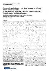
Fig. 1. (a) Top view of the resulting 3D map of the sequence FR1 floor, obtained by concatenating the RGB-D data of each frame in a single point cloud. The resulting map can be used for robot navigation and obstacle avoidance, despite the fact that no SLAM techniques were used in the reconstruction process. (b–f) Some sample images used to build the map are also shown.

The problem of map building and localization can also be solved by Visual Odometry [9,28]. In contrast to Visual SLAM, that allows long term localization by associating visual data with a global map, Visual Odometry systems incrementally estimate frame to frame pose transformations. Consequently, faster computation times are prioritized over localization accuracy. In light of this, mapping and localization with RGB-D sensors can be designed to be both fast and accurate. In this work, a Visual Odometry solution for RGB-D sensors is proposed for indoor mobile robots. By tracking and detecting visual salient features across consecutive frames, the pose (position and orientation) of a moving sensor can be computed in a fast and robust manner with RANSAC [8]. Also, by registering RGB-D data utilizing the respective estimated transformation, a map of the environment is built, as illustrated in Fig. 1. The system is evaluated through

18

B.M.F. Silva and L.M.G. Gon¸calves

a set of experiments carried out on public RGB-D datasets [32] to demonstrate the accuracy and computation performance of the method. In the remaining text, Sect. 2 lists the related works on Visual SLAM and Odometry based on RGB-D sensors. Section 3 describes the inner workings of the proposed system, while the experiments and results are discussed on Sect. 4. Finally, we close the paper in Sect. 5.

2

Related Work

Robot localization is a well studied problem with solutions emerging from research in Simultaneous Localization and Mapping (SLAM). Successful strategies are being achieved with range sensors such as lasers [21] or Time of Flight cameras [19]. Solutions with perspective cameras are also employed in monocular [5] and stereo [13] configurations. The work of Nist´er et al. [22] introduces the “Visual Odometry” terminology, which refers to systems that employ cameras to estimate the position and orientation of a moving agent. This class of systems is generally formed by incremental Structure from Motion [11] approaches that estimate frame to frame pose transformations instead of finding the position relative to a global map (which is the general definition of SLAM). A tutorial paper on the subject was recently pusblished [9,28]. Once unaffordable, depth measurement devices are now being employed in solutions to the localization and mapping problem with the advent of consumer grade RGB-D sensors. These solutions are either dense [16,25,30,35] or feature based [7,12,14,26,31] approaches. Dense solutions [16,25,30,35] directly use the input color/depth data i.e. they do not rely on the extraction and matching of visual features. Steinbruecker et al. [30] propose a method to compute camera motion by estimating the warping transformation between adjacent frames under the assumption of constant image brightness. This work is later complemented [16] to support probabilistic motion models and robust estimators in the transformation estimation, resulting in a system more resilient to moving objects in the scene. Whelan et al. [35] extend the solution of Steinbruecker et al. with a GPU implementation of the algorithm and the incorporation of feature based visual front-ends to the pose estimation process. Osteen et al. [25] take an innovative direction proposing a Visual Odometry algorithm that works by computing correlations between the frequency domain representations of the scene normals. Alternatively, feature based solutions work by matching extracted features between sequential pair of images and then estimating the corresponding transformation through sets of three point matches and RANSAC [8] and/or Iterative Closest Point (ICP) [2]. Henry et al. [12] detect and match FAST [27] features using Calonder descriptors [4] and optimize an error function with RANSAC and a non-linear version of ICP. After detecting loop closures, Bundle Adjustment [33] or graph optimization [10] is executed to ensure global pose consistency. Paton and Kosecka [26] and Hu et al. [14] propose a similar system, although the latter has a strategy to switch between the algorithm of Henry et al. and a

Visual Odometry with RGB-D Cameras

19

Fig. 2. The proposed Visual Odometry method.

pure monocular Visual Odometry algorithm. This strategy is employed to deal with situations in which the available depth data is not sufficient. The detection and extraction of sparse visual features was also the direction taken by Endres et al. When designing RGB-D SLAM [7], which works by extracting SIFT features [18] on a GPU implementation and optimizing the pose graph with g2o [17]. Finally, St¨ uckler and Benhke [31] employ a surfel representation of the scene containing depth and color statistics which are later matched and registered in a multi-resolution scheme. Our work relies on sparse visual features and incremental pose estimation between adjacent frames. However, in contrast to all mentioned solutions of this class, we do not employ tracking by detection in frame to frame matching. Instead of extracting keypoints and matching them using their descriptors, we track features using a short baseline optical flow tracker. As evidenced by the experiments, the system can rapidly estimate accurate camera poses without the need of using state-of-the-art GPUs.

3 3.1

Proposed System Overview

Our goal is to estimate the pose (position and orientation) of a moving sensor (a Kinect style RGB-D camera) using only the captured color and depth information. Camera poses are estimated relative to the first RGB-D frame (the origin reference frame). A map consisting of all registered RGB-D frames is also computed at each time step. The proposed system tracks visually salient features across consecutive image pairs It−1 , It , adds keypoints on an as-needed basis and then robustly estimates the camera pose [Rt |tt ] using the feature points. Each step of the algorithm, depicted on Fig. 2, is explained as follows. 3.2

Tracking Visual Features

At the initial time step (frame I0 ), Shi-Tomasi corners [29] are extracted and invalid keypoints (points without a depth measurement) are removed. ˆ = [x, y, d]t , The remaining points form the initial set of features {ˆ x}0 , with x where d is the depth of the point at image coordinates x, y. Then, for each frame x}t are tracked through sparse multiscale It with t > 0, the points of the set {ˆ optical flow [3], assuming a small capture interval between It−1 and It and image brightness held constant. Since a point can become lost (or invalid) after tracking, invalid points are removed once again. Then, the resulting set of tracked

20

B.M.F. Silva and L.M.G. Gon¸calves

points {x}t and the set with the corresponding points on the previous time step {x}t−1 are used to estimate the current camera pose [Rt |tt ], as explained in Sect. 3.3. We proceed with the following strategy for the management of keypoints being currently tracked. Instead of detecting and adding keypoints only when the number of tracked keypoints is below a threshold, we extract Shi-Tomasi corners at every frame, although each keypoint is only added to the tracker if two conditions are met: the current number of active keypoints is below a threshold τ and the keypoint lies in a region in the image without any tracked point. ˆ of the set of newly extracted points {ˆ To accomplish this, every point p p}t is checked to test whether it lies inside any of the rectangular perimeter Wj ˆ is not inside any centered around each tracked point xj of the set {x}t . If p rectangular region, it is added to the tracker in the set {p}t . Note that it can only be used to estimate the camera pose on the next frame, since it does not have a correspondence at t − 1 yet. Points with invalid depth measurements once again discarded. This process is illustrated in Fig. 3.

Fig. 3. Feature tracking strategy: (a) At I0 , the initial set of features {ˆ x}0 (blue crosses) x}t (gray crosses) is tracked into {x}t (blue crosses). is extracted. (b) At It with t > 0, {ˆ Keypoints that could not be tracked are shown in yellow. (c) The set of added keypoints {p}t is shown with green crosses, whereas the rejected points, which are within the rectangular perimeter (dashed rectangles) of the tracked points, are shown with red crosses (Color figure online).

By varying the maximum number of active points τ and the size of the rectangular windows Wj , different configurations of the algorithm can be achieved, allowing tuning based on application requirements (such as accuracy or performance). 3.3

Frame to Frame Motion Estimation

The sets containing all tracked points in the current {x}t and in the previous frame {x}t−1 are used to estimate the camera pose [Rt |tt ]. For this, points are reprojected to 3D as ⎤ ⎡ ⎤ ⎡ d(x − cx )/fx X ⎣ Y ⎦ = ⎣ d(y − cy )/fy ⎦, d Z

Visual Odometry with RGB-D Cameras

21

resulting in the sets {X}t and {X}t−1 of 3D points referenced in the camera frames of It and It−1 respectively. The terms fx , fy , cx , cy are the intrinsic parameters of the Kinect RGB sensor. The current camera pose can be estimated by finding the rigid transformation [R∗ |t∗ ] that minimizes in the least squares sense the alignment error in 3D space between the two point sets, as shows Eq. 1. We proceed with the method proposed by Umeyama [34] which uses Singular Value Decomposition to solve for the transformation parameters.    ||Xit−1 − RXit + t ||2 (1) R∗ , t∗ = argmin R,t

i

Since point correspondences Xit , Xit−1 can be falsely estimated (due to occlusions, bad lighting conditions, the aperture problem inherent to optical flow, etc.), a robust pose estimator should be employed to compute the desired transformation. The RANSAC [8] algorithm accomplishes this function. RANSAC works by sampling a minimal set of data to estimate a model, which in our case are point correspondences and a camera transformation respectively. For a given number of iterations, minimal sets of three point matches are randomly chosen to estimate a hypothesis pose by minimizing Eq. 1. All other point correspondences are then used to count the number of inliers (correspondences with alignment error below a specified threshold ). The hypothesis with the largest number of inliers is elected as the winner transformation. Using all the inliers corresponding to the winner solution, a new least squares transformation is computed, resulting in the sought [Rt |tt ]. This last step results in camera poses significantly better than simply taking the R and t related to the winner transformation and the performance penalty is negligible. The RANSAC algorithm can run faster by using an adaptive termination of the procedure that takes into account an estimate of the fraction of inlier correspondences [8]. Hence, by updating this fraction with the largest ratio found after each iteration of the algorithm, a significant speedup is achieved. The last step in our algorithm involves registering the RGB-D frame It with that of It−1 . The estimated pose is used to transform the 3D points in the current camera frame to the reference frame relative to the previous camera by applying the [Rt |tt ] to each point of {X}t . By doing so, the current transformation is always estimated relative to the origin reference frame and a map formed by all registered RGB-D frames until time step t is computed. 3.4

Algorithm Parameterization

In the current implementation, all rectangular regions Wj of the tracked points have a fixed size. All experiments of Sect. 4 are executed with maximum number of tracked points τ = 1000 and window Wj with size 30 × 30. RANSAC parameters are set with a correspondence error threshold  of 8 mm (which automatically rejects the imprecise measurements for features with large depth) and a maximum of 10000 iterations. The reported values for all parameters were found after running the algorithm through several initial experiments.

22

B.M.F. Silva and L.M.G. Gon¸calves

4

Experiments and Results

4.1

Methodology

The proposed Visual Odometry system is evaluated with respect to its localization accuracy and computational performance. All experiments were carried out on a desktop PC with an Intel Core i5 3470 3.2 GHz processor and 8 GB of RAM running on Ubuntu Linux 12.04. The system is implemented in C++ using Point Cloud Library [23] and OpenCV [24]. We note that the OpenCV library provides a parallelized implementation of the optical flow algorithm based on Threading Building Blocks [15], a multithread library that was key to achieve the reported performance of the algorithm. We resort to the datasets and benchmark proposed by Sturm et al. [32] to evaluate our system. Using the provided RGB-D data (with synchronized ground truth collected by a motion capture system), we assess the localization accuracy of the proposed system by estimating the translational and rotational Relative Positioning Error (RPE). The RPE is a performance metric suitable to Visual Odometry systems since it gives a measure of the drift (accumulated error) per unit of time. Accordingly, we report the Root Mean Square Error (RMSE) between all possible pairs of consecutive frames Ii , Ii+1 , provinding thus a robust statistic of all estimated trajectories. The same error statistics are also computed for the RGB-D SLAM system [7] to clarify how the proposed system compares against state-of-the-art algorithms in RGB-D localization. The results from RGB-D SLAM are available at the website from the authors of the benchmark used in the experiments1 . A total of eight datasets having different characteristics such as linear and angular camera velocities, total trajectory length and number of input frames on different scenes were selected for the experiments. All of the chosen image sequences were captured by a sensor hand-held by a moving person and have plenty of texture from which visual features can be extracted. The details about the image sequences are shown in Table 1. 4.2

Accuracy

Exploiting the fact that the RPE gives independent measurements for the translational and rotational motion estimation, the results after executing the algorithm on each image sequence are presented on two different tables, Tables 2 and 3. The RMSE and maximum translational and rotational error accumulation per frame are shown for both the proposed system and RGB-D SLAM. The proposed Visual Odometry system shows superior or equivalent accuracy regarding the RMSE translational and rotational drifts per frame compared to RGB-D SLAM. Error reductions in the translational RMSE varies between 0.3 mm (on FR1 XYZ ) to 14.4 mm (FR1 plant), which represents respectively an 1

https://svncvpr.in.tum.de/cvpr-ros-pkg/trunk/rgbd benchmark/rgbd benchmark tools/data/rgbdslam/.

Visual Odometry with RGB-D Cameras

23

Table 1. Details of the datasets used in the experiments. Sequence

Length

Frames Avg. Transl. Vel Avg. Ang. Vel

9.236 m

573

0.413 m/s

23.327◦ /s

FR1 desk2 10.161 m

620

0.426 m/s

29.308◦ /s

FR1 room 15.989 m 1352

0.334 m/s

29.882◦ /s

FR1 floor

12.569 m

979

0.258 m/s

15.071◦ /s

FR1 XYZ

7.029 m

792

0.058 m/s

8.920◦ /s

18.880 m 2893

0.193 m/s

6.338◦ /s

FR1 plant 14.795 m 1126

0.365 m/s

27.891◦ /s

FR1 teddy 15.709 m 1401

0.315 m/s

21.320◦ /s

FR1 desk

FR2 desk

Table 2. Comparison between the proposed system and the state-of-the-art implementation of RGB-D SLAM. Shown are the RMSE and maximum translational Relative Positioning Error, which gives the resulting drift in meters per frame. Best results are in boldface. Translational relative positioning error (m/frame) Sequence

Prop. System

FR1 desk

0.0105 m (0.0476 m) 0.0117 m (0.0630 m)

10.2 %

FR1 desk2 0.0101 m (0.0508 m) 0.0175 m (0.2183 m)

42.2 %

FR1 room 0.0096 m (0.1100 m) 0.0137 m (0.1590 m)

29.9 %

FR1 floor

0.0030 m (0.0141 m) 0.0037 m (0.0271 m)

18.9 %

FR1 XYZ

0.0054 m (0.0203 m) 0.0057 m (0.0212 m)

5.2 %

FR2 desk

0.0039 m (0.0164 m) 0.0047 m (0.0685 m)

17.0 %

FR1 plant 0.0063 m (0.0715 m) 0.0207 m (0.1210 m)

69.5 %

FR1 teddy 0.0194 m (0.1836 m)

RGB-D SLAM

Improvement

0.0254 m (0.1094 m) 23.6 %

Table 3. Comparison between the proposed system and the state-of-the-art implementation of RGB-D SLAM. Shown are the RMSE and maximum rotational Relative Positioning Error, which gives the resulting drift in degrees per frame. Best results are in boldface. Rotational relative positioning error (◦ /frame) Sequence

Prop. System

RGB-D SLAM Improvement

FR1 desk

0.5378 2.0777 0.7309 6.8548 26.4 %

FR1 desk2 0.5464 3.1128 1.0665 9.6320 48.7 % FR1 room 0.4057 1.9463 0.6319 5.1501 35.7 % FR1 floor

0.2418 1.7575 0.2833 1.9288 14.6 %

FR1 XYZ

0.3380 1.0935 0.3529 1.6332

4.2 %

FR2 desk

0.2712 1.2527 0.2999 2.4685

9.5 %

FR1 plant 0.3592 2.1466 1.2550 4.1202 71.3 % FR1 teddy 0.5900 4.6240 1.4490 7.2330 59.2 %

24

B.M.F. Silva and L.M.G. Gon¸calves

Fig. 4. Camera path computed by the proposed Visual Odometry algorithm (shown in blue) in comparison to the ground truth trajectory (shown in black). The red lines are the distance between the computed and ground truth positions for corresponding time steps, which were equally sample at every 10 frames (Color figure online).

Visual Odometry with RGB-D Cameras

25

improvement of 5.2 % and 69.5 % over the compared algorithm. Similar results also hold for the rotational error, with improvements ranging from 4.2 % (on FR1 XYZ ) up to 71.3 % (on FR1 plant). On average, the RMSE translational and rotational RPEs are 8.5 mm/frame and 0.411◦ /frame for the proposed system and 12.8 mm/frame and 0.758◦ /frame for RGB-D SLAM, although loop closures and drift minimization are not employed as does RGB-D SLAM. Figure 4 shows the resulting camera trajectory computed by the proposed system along with the ground truth trajectory and positional error for equally sampled time steps. Remarkably, the proposed system shows accurate localization on several adverse situations. The camera pose can be computed with good accuracy on image sequences with high speed camera movement (and thus considerable amounts of motion blur) and even on sequences consisting on a large number of frames and traveled distances. 4.3

Computational Performance

The performance of the proposed algorithm is assessed by collecting the total time spent on the execution of each RGB-D frame. The average, standard deviation and maximum time per frame are shown in Table 4. Figure 5 depicts the running time of each image sequence used in the experiments. The resulting running times for the proposed algorithm stays in an stable margin during most of the time, as can be noticed from the reported running times and standard deviations. Despite the fact that no specialized hardware (e.g. modern GPUs) is used by our system, the camera pose can be computed at more than 36 Hz, as evidenced by the computed average over all sequences (27.346 ms per frame). The slowest time spent on a single frame (∼170 ms) is still faster than the reported average of RGB-D SLAM (330/350 ms without/with global optimization respectively) [7] and is still fast enough for doing real-time Table 4. Performance of the proposed RGB-D Visual Odometry system. Shown are the average, standard deviation and maximum running times computed over all frames of each sequence. Sequence

Avg

FR1 desk

25.041 ms

4.988 ms 101.109 ms

FR1 desk2 25.642 ms

9.558 ms 137.624 ms

FR1 room 24.304 ms

4.072 ms

FR1 floor

34.217 ms

8.548 ms 103.023 ms

FR1 XYZ

22.573 ms

1.521 ms

30.905 ms

FR2 desk

23.127 ms

1.629 ms

39.451 ms

FR1 plant 26.767 ms

Std. dev

Max

66.056 ms

6.334 ms 131.797 ms

FR1 teddy 37.097 ms 22.962 ms 171.980 ms Total avg

27.346 ms

26

B.M.F. Silva and L.M.G. Gon¸calves

Fig. 5. Running times for each image sequence used in the evaluation of the proposed system. The varying quantity of extracted and tracked features and oscillations in the RANSAC runtime explain the peaks in the estimated timings collected among different sequences.

Visual Odometry with RGB-D Cameras

27

vision based applications (∼7 Hz). The varying quantity of extracted and tracked features and oscillations in the RANSAC runtime explain the peaks in the estimated timings collected among different sequences. Specifically on the sequence FR1 floor, a large number of keypoints is tracked in each frame due to the large amount of texture in the scene, which results in an almost uniform sampling of points for tracking and thus in a higher execution time. 4.4

Qualitative Results

We also show qualitative results of the proposed Visual Odometry method. Two resulting 3D maps are shown in Figs. 1 and 6, along with image samples of the respective sequences. A third reconstruction is illustrated on Fig. 7 depicting the result of our system after processing our own datasets. For this, 217 RGB-D frames captured at the Natalnet Laboratory (situated at the Department of Computer Engineering and Automation from the Federal University of Rio Grande do Norte) were supplied to the algorithm. These maps are built in a straightforward manner by simply transforming and concatenating the RGB-D data corresponding to each frame in a globally registered point cloud. The maps show local consistency and very few noticeable registration errors, even though no global optimization is performed. The resulting point cloud can be post processed and then employed in a number of applications such as an

Fig. 6. (a) 3D map of the sequence FR1 desk2, obtained by concatenating the RGB-D data of each frame in a single point cloud with 1 cm resolution. The algorithm runs in real-time and is robust against fast camera movements. Note the quality of the map, despite the fact that no SLAM techniques were used in the reconstruction process. (b–f) Some sample images used to build the map (some of them showing noticeable motion blur).

28

B.M.F. Silva and L.M.G. Gon¸calves

in-hand scanner for object and environment digitalization and also for robot navigation and obstacle avoidance. Additionally, we supply videos of our algorithm processing selected sequences on the YouTube page of the author2 .

Fig. 7. (a) 3D reconstruction of the Natalnet laboratory computed by the proposed algorithm. Each RGB-D frame is concatenated in a globally registered point cloud with voxels of 1 cm resolution. (b–f) Some sample images used in the reconstruction.

4.5

Algorithm Limitations

In the current implementation, the proposed algorithm has two main limitations: (a) processing textureless images; and (b) processing images without depth measurements. Therefore, the use of the system in its current state is restricted to texture rich indoor environments. The former limitation can be tackled by employing strategies to detect textureless environments and then switching to registration methods on range data, as performed by the work of Henry et al. [12]. The latter limitation is inherent to range based methods and can be overcomed with solutions from the monocular Visual Odometry literature.

5

Conclusion

In this work, we propose a Visual Odometry system based on RGB-D sensors that estimates camera poses using appearance/depth measurements. At each 2

https://www.youtube.com/user/brunomfs/videos.

Visual Odometry with RGB-D Cameras

29

RGB-D frame, visual features are detected and tracked through sparse optical flow with new features being added if they do not fall within regions related to already tracked features. Camera poses computed as the transformation between adjacent frames using RANSAC can then be estimated in a fast and accurate manner. The accuracy and computational performance of the proposed system is demonstrated by experiments carried out on public available RGB-D datasets and benchmark [32] and a comparison with the state-of-the-art RGB-D SLAM algorithm [7] is presented to clarify how competitive is our proposal. The average RMSE translational and rotational RPE are 8.5 mm/frame and 0.411◦ /frame for the proposed system and 12.8 mm/frame and 0.758◦ /frame for RGB-D SLAM, at the same time that the running times for the proposed algorithm are almost one order of magnitude faster on average. This results are achieved without the use of expensive and specialized hardware such as modern GPUs. The proposed Visual Odometry and mapping algorithm can be employed in a number of important applications related to real-time 3D reconstruction and Robotics, such as object digitalization, indoor mapping and robot navigation. Future works will focus on detcting loop closures and trajectory optimization algorithms using the Visual Odomety module as a front-end in a full SLAM solution. Acknowledgments. This work is supported by the Coordination for the Improvement of Higher Education Personnel (CAPES) and the Funding Agency for Studies and Projects (FINEP).

References 1. Aldoma, A., Marton, Z., Tombari, F., Wohlkinger, W., Potthast, C., Zeisl, B., Rusu, R., Gedikli, S., Vincze, M.: Tutorial: point cloud library: three-dimensional object recognition and 6 DOF pose estimation. Robot. Autom. Mag. 19(3), 80–91 (2012) 2. Besl, P., McKay, N.D.: A method for registration of 3-D shapes. IEEE Trans. Pattern Anal. Mach. Intel. 14(2), 239–256 (1992) 3. Bouguet, J.Y.: Pyramidal implementation of the lucas kanade feature tracker. Intel Corporation, Microprocessor Research Labs (2000) 4. Calonder, M., Lepetit, V., Fua, P.: Keypoint signatures for fast learning and recognition. In: Forsyth, D., Torr, P., Zisserman, A. (eds.) ECCV 2008, Part I. LNCS, vol. 5302, pp. 58–71. Springer, Heidelberg (2008) 5. Davison, A.: Real-time simultaneous localisation and mapping with a single camera. In: Proceedings of IEEE International Conference on Computer Vision (ICCV) (2003) 6. Du, H., Henry, P., Ren, X., Cheng, M., Goldman, D., Seitz, S., Fox, D.: Interactive 3D modeling of indoor environments with a consumer depth camera. In: Proceedings of the International Conference on Ubiquitous Computing (UbiComp). ACM, New York (2011) 7. Endres, F., Hess, J., Engelhard, N., Sturm, J., Cremers, D., Burgard, W.: An evaluation of the RGB-D SLAM system. In: Proceedings of IEEE International Conference on Robotics and Automation (ICRA), St. Paul, MA, USA, May 2012

30

B.M.F. Silva and L.M.G. Gon¸calves

8. Fischler, M., Bolles, R.: Random sample consensus: a paradigm for model fitting with applications to image analysis and automated cartography. Commun. ACM 24(6), 381–395 (1981) 9. Fraundorfer, F., Scaramuzza, D.: Visual odometry: part ii: matching, robustness, optimization, and applications. IEEE Robot. Autom. Mag. 19(2), 78–90 (2012) 10. Grisetti, G., Stachniss, C., Burgard, W.: Nonlinear constraint network optimization for efficient map learning. IEEE Trans. Intel. Transp. Syst. 10(3), 428–439 (2009) 11. Hartley, R.I., Zisserman, A.: Multiple View Geometry in Computer Vision, 2nd edn. Cambridge University Press, Cambridge (2004) 12. Henry, P., Krainin, M., Herbst, E., Ren, X., Fox, D.: RGB-D mapping: using kinectstyle depth cameras for dense 3D modeling of indoor environments. Int. J. Robot. Res. 31(5), 647–663 (2012) 13. Howard, A.: Real-time stereo visual odometry for autonomous ground vehicles. In: Proceedings of IEEE/RSJ International Conference on Intelligent Robots and Systems (IROS) (2008) 14. Hu, G., Huang, S., Zhao, L., Alempijevic, A., Dissanayake, G.: A robust RGB-D SLAM algorithm. In: Proceedings of IEEE/RSJ International Conference on Intelligent Robots and Systems (IROS), pp. 1714–1719 (2012) 15. Intel: Threading Building Blocks (TBB) (2014). https://www.threadingbuilding blocks.org/home. Accessed 1 October 2014 16. Kerl, C., Sturm, J., Cremers, D.: Robust odometry estimation for RGB-D cameras. In: Proceedings of IEEE International Conference on Robotics and Automation (ICRA), May 2013 17. Kummerle, R., Grisetti, G., Strasdat, H., Konolige, K., Burgard, W.: G2O: a general framework for graph optimization. In: Proceedings of IEEE International Conference on Robotics and Automation (ICRA), pp. 3607–3613 (2011) 18. Lowe, D.: Distinctive image features from scale-invariant keypoints. Int. J. Comput. Vis. 60(2), 91–110 (2004) 19. May, S., Droeschel, D., Holz, D., Fuchs, S., Malis, E., N¨ uchter, A., Hertzberg, J.: Three-dimensional mapping with time-of-flight cameras. J. Field Robot. 26(11– 12), 934–965 (2009) 20. Microsoft: Microsoft Kinect (2014). http://www.xbox.com/en-US/kinect. Accessed 1 October 2014 21. Newman, P., Cole, D., Ho, K.: Outdoor SLAM using visual appearance and laser ranging. In: Proceedings of IEEE International Conference on Robotics and Automation (ICRA), pp. 1180–1187 (2006) 22. Nist´er, D., Naroditsky, O., Bergen, J.: Visual odometry. In: Proceedings of IEEE Computer Society Conference on Computer Vision and Pattern Recognition (CVPR), pp. 652–659 (2004) 23. Open Perception: Point Cloud Library (PCL) (2014). http://pointclouds.org. Accessed 1 October 2014 24. OpenCV Foundation: OpenCV Library (2014). http://opencv.org. Accessed 1 October 2014 25. Osteen, P., Owens, J., Kessens, C.: Online egomotion estimation of RGB-D sensors using spherical harmonics. In: Proceedings of IEEE International Conference on Robotics and Automation (ICRA), pp. 1679–1684 (2012) 26. Paton, M., Kosecka, J.: Adaptive RGB-D localization. In: Conference on Computer and Robot Vision (CRV), pp. 24–31 (2012) 27. Rosten, E., Drummond, T.W.: Machine learning for high-speed corner detection. In: Leonardis, A., Bischof, H., Pinz, A. (eds.) ECCV 2006, Part I. LNCS, vol. 3951, pp. 430–443. Springer, Heidelberg (2006)

Visual Odometry with RGB-D Cameras

31

28. Scaramuzza, D., Fraundorfer, F.: Visual odometry [tutorial]. IEEE Robot. Autom. Mag. 18(4), 80–92 (2011) 29. Shi, J., Tomasi, C.: Good features to track. In: Proceedings of IEEE Conference on Computer Vision and Pattern Recognition (CVPR), pp. 593–600 (1994) 30. Steinbruecker, F., Sturm, J., Cremers, D.: Real-time visual odometry from dense RGB-D images. In: Workshop on Live Dense Reconstruction with Moving Cameras at the International Conference on Computer Vision (ICCV) (2011) 31. St¨ uckler, J., Behnke, S.: Integrating depth and color cues for dense multi-resolution scene mapping using RGB-D cameras. In: Proceedings of IEEE International Conference on Multisensor Fusion and Information Integration (MFI), September 2012 32. Sturm, J., Engelhard, N., Endres, F., Burgard, W., Cremers, D.: A benchmark for the evaluation of RGB-D SLAM systems. In: Proceedings of IEEE/RSJ International Conference on Intelligent Robot Systems (IROS), October 2012 33. Triggs, B., McLauchlan, P.F., Hartley, R.I., Fitzgibbon, A.W.: Bundle adjustment – a modern synthesis. In: Triggs, B., Zisserman, A., Szeliski, R. (eds.) ICCV-WS 1999. LNCS, vol. 1883, pp. 298–372. Springer, Heidelberg (2000) 34. Umeyama, S.: Least-squares estimation of transformation parameters between two point patterns. IEEE Trans. Pattern Anal. Mach. Intel. 13(4), 376–380 (1991) 35. Whelan, T., Johannsson, H., Kaess, M., Leonard, J., McDonald, J.: Robust realtime visual odometry for dense RGB-D mapping. In: Proceedings of IEEE International Conference on Robotics and Automation (ICRA), Karlsruhe, Germany, May 2013

http://www.springer.com/978-3-662-48133-2