Visual Training and Classification of Textured Scene Images - CiteSeerX

Visual Training and Classification of Textured Scene Images Markus Turtinen and Matti Pietik¨ainen Department of Electrical and Information Engineering Machine Vision Group, Infotech Oulu P.O. Box 4500, FIN-90014 University of Oulu, FINLAND Email: [email protected], [email protected] Telephone: +358-8-533 2796, Fax: +358-8-533 2796

Abstract— Classification of textures in scene images is very difficult due to the high variability of the data within and between images caused by effects such as non-homogeneity of the textures, changes in illumination, shadows, foreshortening and self-occlusion. For these reasons, finding proper features and representative training samples for a classifier is very problematic. Even defining the classes which can be discriminated with texture information is not so straightforward. In this paper, a visualization-based approach for training a texture classifier is presented. Powerful local binary patterns (LBP) are used as texture features and a self-organizing map (SOM) is employed for visual training and classification, providing very promising results in the classification of outdoor scene images.

I. I NTRODUCTION The analysis of 3D-textured real-world images has recently been a topic of increasing interest due to many potential applications. These include, for example, classification and inspection of materials or objects from varying viewpoints, classification and segmentation of scene images e.g. for navigation purposes, aerial image analysis, and retrieval of scene images from multimedia databases. Analysis of outdoor scene images, for example for navigating a mobile robot, is very challenging. Texture could play an important role in this kind of application, because it is much more robust than color with respect to changes in illumination and it could also be utilized in night vision [1]. Castano et al. argued that classification is a more important issue in the vast majority of applications rather than clustering or unsupervised segmentation. Regardless of its importance, texture classification has been rarely utilized. Setchell and Campbell [2] used color Gabor texture features for classifying pre-labeled regions from images in the Bristol Image Database [3]. Castano et al. assessed the performance of two Gabor filtering based texture classification methods on a number of real-world images relevant to autonomous navigation on crosscountry terrain and to autonomous geology [1]. They obtained satisfactory results for rather simple terrain images containing four classes (soil, trees, bushes/grass, and sky), but the results for the rock dataset were much poorer. Recently, Pietik¨ainen et al. applied local binary pattern (LBP) texture features [4] to the classification of scene images taken by a person walking along a street [5]. Five texture classes were defined: sky, trees, grass, road and buildings. A

view-based classification method using multiple LBP distributions as texture models provided an accuracy of up to 85%. They also applied the same methodology to the classification Columbia-Utrecht database (CUReT) textures imaged under different viewpoints and illuminations, exceeding the performance obtained by earlier studies [6]. Outdoor scene image analysis sets high requirements for the features used. There are wide illumination variations even in a single image and for example, the influences of shadowing and overall illumination on classification performance should be considered. Also the foreshortening effect and nonhomogeneity of objects set extra requirements for the features. Even without these problems the scene classification is difficult because of the great variability within classes; consider for example different kinds of trees. The variation between classes also changes greatly. For example, in some scenes the grass can resemble a road in a certain illumination, but on the other hand it can also look like the leaves of trees in some other aspect. Because of these hard conditions and problems, a tool for selecting classes, features and representative training samples would be highly desirable. Recently, a method based on visual training has provided a significant breakthrough in wood inspection performance [7]. It combines an intuitive user interface with an unsupervised classifier. The idea is to project the unlabeled training data into two dimensions with some dimensionality reduction method like a self-organizing map (SOM) [8]. Then the training data is visualized on the 2D map where the user determines the boundaries between classes. The approach does not require labeling of separate samples, which is often an inconsistent and error prone task reducing the accuracy required. The decision of the class boundaries is based on observing the data set as a whole, utilizing visualization and clustering of the data. A similar SOM-based method using LBP texture features has provided outstanding results in paper characterization [9]. A visualization-based approach could also be very useful in the training of a classifier for 3D scene analysis. Most of the research, however, has not paid much attention to the significant roles of the training sample and feature selection in these applications. In [5], an approach for learning appearance models for view-based recognition using self-organization of feature distributions was introduced and applied to the

recognition of CUReT textures. In this paper, we will explore the use of visual training and classification in the analysis of outdoor scene images. Separate training and testing sets are used in the experiments. The images to be analyzed are divided into small non-overlapping blocks, and distributions of LBP features are computed within each block. LBP distributions are then fed to a self-organizing map for clustering the high-dimensional feature data on a twodimensional map. The visualization of the SOM is used for selecting a representative training set for classification. In the testing phase, the classification of image blocks is done with either a SOM-based or a k-NN classifier. In addition to the training set selection, the developed tool can also be used for evaluating the performance of chosen texture features. The approach presented is experimentally evaluated with a set of outdoor scene images taken from the Outex database [10]. The classification performance is determined by classifying pre-labeled ground truth regions, but also examples of segmenting the whole images are shown. II. A NALYSIS T OOL Fig. 1 shows a block diagram of the analysis method used. First the original image is divided into non-overlapping blocks of a chosen size. The texture features are extracted within each block and used as an input for the self-organizing map. The two-dimensional SOM obtained is then used for selecting the training data for classification. The user can also see from the map how well the chosen texture features can discriminate different classes into separate clusters, and try again with other features if the discrimination is not good enough. In the testing phase, the classification performance of selected features is determined with an independent data set.

Training images

Division to sub images

Feature extraction

SOM Visualization

Selecting training data

Testing images

Fig. 1.

Feature analysis

Classification SOM

Block diagram of analysis method

A. Texture Feature Extraction For the present implementation, we chose the local binary pattern operator, which has shown excellent performance in

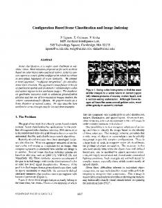
the classification of 2D [4] and 3D [5] textures. LBP is a gray-scale invariant texture primitive statistic. This is a very important property, because the scene textures tend to have significant local and global gray-scale variations. The LBP features are also very fast to compute allowing processing at video rates. For each pixel in an image, a binary code is produced by thresholding its neighborhood with the value of the center pixel. A histogram is created to collect up the occurrences of different binary patterns. The basic version of the LBP operator considers only the eight neighbors of a pixel, but the definition can be extended to include all circular neighborhoods with any number of pixels [4]. By extending the neighborhood one can collect larger-scale texture primitives. In our research, we considered neighborhoods with 8, 16 and 24 samples and radii 1, 3 and 5. In order to reduce the number of bins needed, we adopted the ”uniform” pattern approach proposed in [4]. The operators chosen were ”rotationdependent” operators LBPu2 8,1 (uniform, 8 samples; radius 1) and multiresolution LBPu2 8,1+16,3+24,5 (uniform; 8, 16 and 24 samples; radii 1, 3 and 5). The multiresolution operator is obtained by concatenating histograms produced by operators at three resolutions into a single histogram. B. Visual Training and Feature Analysis The self-organizing map is used to reduce the dimensionality of the feature data. In dimensionality reduction, the data is projected to a two-dimensional space and clustered according to similarity [8]. Similar texture features cluster close to each other, while more distant ones construct their own node clusters on the SOM grid. Fig. 2 illustrates the principle of SOM-based visual training and feature analysis in scene analysis. Each sub-image (block) extracted from the original scene image is considered as a separate sample. Texture feature vectors (= LBP histograms) derived from these samples are then used as input for the SOM. After training the SOM, we visualize it and select a few nodes from the visualized map for further analysis. A new smaller-sized SOM is then trained by using selected samples representing given class(es) as its input. Visualizing this new SOM reveals if there are samples from some other classes mixed with the class under consideration. The nodes, and samples inside them, representing each correct class are then selected and labeled to be included in the training set of the classifier. The following steps summarize how the visual training is performed and Fig. 3 shows a real-world example of actual visualization parts. The original training images can be used as help when rejecting nodes, but usually rejection can be done directly based on the appearance of nodes. 1) Divide training images to small sub-images and calculate features from these small images. 2) Train a self-organizing map with these features. 3) Visualize the map and select nodes with similar appearance.

s

t

tree

sky

grass grass road

road

grass

road

tree

g r

b scene image

g

sky

tree tree

SOM mapping samples back to the original scece: feature analysis add to training set

tree

not tree

tree

tree

Select nodes representing the class ’grass’ and train a new SOM with these samples

feature analysis Fig. 2.

SOM-based visual training

4) Train a new smaller map with samples inside the selected nodes. 5) Visualize the smaller SOM and reject nodes representing samples from other classes. All other sampes are added to the training set and labeled similarly. 6) Goto step 3 until all classes have been gone through. Feature analysis is also made in this phase. By selecting a group of nodes and mapping samples inside them back to the original image, we can see if the features can discriminate this data well. We can, for example, select a group of nodes assumed to represent trees in the scene and see how the samples inside these nodes are actually located in the original image. If different classes construct compact clusters and do not mix too much with the other classes, we can make an assumption that the chosen features are good enough. Otherwise, if the nodes of the class ’tree’, for example, are spread all over the SOM and different classes are mixed badly inside nodes, we can assume that the features cannot separate the classes in question well enough. Fig. 4 shows a real-world example of how the feature analysis and visualization of clustering work. The images are shown to the user with full color, even though the texture features were extracted after gray scale conversion. For a human it is much easier to discriminate details from color than gray scale images. The upper part of the figure shows a SOM with selected nodes assumed to represent the class ’tree’, and the lower part shows the original scene image. Those samples that are selected from the SOM are also selected in the original image. We can see that the features work quite well, because the cluster is compact in the SOM and also the mixture with other classes is small. C. Classification In the present system, the classification is made either with a SOM-based approach or with a k-NN classifier. The chosen

Select suspicious nodes and map them back to the training image

Samples inside selected nodes seem to belong to the class ’road’, so they can be rejected Fig. 3.

Visual training example

classifier utilizes the labeled training set constructed in the training and feature analysis phase. Some details about the SOM classifier are given below. The label for each node in the SOM is selected in such a way that each node gets the same label as the majority of the training samples in that node. The nodes getting no training samples are labeled by finding the nearest training sample. Instead of the Euclidean distance normally used with SOM, we used a log-likelihood statistic for finding the nearest node and sample in the training of the SOM and in classification. This distance measure has performed very well in the earlier

SOM with selected nodes

Mapping selected samples back to the scene Fig. 4.

Visual feature analysis

studies with LBP features [4]. The log-likelihood statistic is calculated as: L(S, M ) =

B X

Sb log Mb ,

(1)

b=1

where S and M are the sample and model distributions, B is the number of bins and Sb and Mb correspond to the sample and model probabilities at bin b [4]. In the classification stage, the image to be analyzed is first divided into blocks as in the training phase. Each block is then classified with a SOM, and as a result a segmented image is generated and displayed. Classification is simple: samples are compared directly to the nodes of the SOM and the closest nodes are found. The performance of the classification can be determined considering only blocks located inside pre-labeled ground truth regions. The classification could also be made pixel-wise by centering a circular disk with a radius of chosen size at the pixel being classified. Then we compute the sample feature histogram over the disk, and assign the pixel to the class whose model is most similar to the sample. III. E XPERIMENTS The same data set as in [5] was used, where image classification was done pixel-wise using a circular disk with a radius of 30 pixels at the pixel being classified. First the scenes were divided into ground-truth regions (sky, trees, grass, road and buildings) by hand and model LBP distributions for each class were determined. In classification, a pixel was assigned to the class whose model was most similar to the sample. The block-based classification used in our present experiments is rougher than the pixel-based one, but it makes

real-time processing possible. The block size affects the segmentation resolution in such a way that the width of the block (N ) is basically the smallest distance between different segments or classes that can be detected. In the case of texturebased classification, this approach still leads to a rather good resolution when the original images are very large compared to the blocks. The image data consisted of a sequence of 22 outdoor scene images of 2272x1704 pixels. The set is available at the Outex database [10] in the test suite ID Outex NS 00001 (see http://www.outex.oulu.fi). The chosen block size was 64x64 pixels, and therefore we had 910 (= 35x26) blocks from each scene. The remaining 32 pixels from the left and 40 pixels from the bottom of each image were left out because they did not fit in the blocks. We selected the LBPu2 8,1 operator, which gave rather good results also in [5] (80.92 %). In addition, LBPu2 8,1+16,3+24,5 was used, obtaining an 85.43 % accuracy in the previous study. The training set was created scene by scene. First, a SOM of its own was built for each scene image. Then, the areas representing a specific class were selected from each SOM and a new SOM was created using this selected data. This was repeated for all classes to be considered. The SOMs representing all scenes and classes were then combined to form the final training set for the classifier. A feature analysis was also made for each scene separately. Fig. 5 shows an example how the texture operators used cluster the ’road’ class from the training image P9100032. We can see that ’road’ is mixed quite often to the class ’grass’. The textures of ’road’ and ’grass’ resemble each other even though they differ much in color. Also the ’road’ and ’grass’ clusters in SOM are very close to each other and partly mixed. Fig. 5 also shows how LBPu2 8,1 can discriminate the class ’sky’. Now the confusion with the other classes is very small, and the cluster in the SOM is more compact (see the nodes in the upper right corner of LBPu2 8,1 SOM). It is clear that the use of small image blocks instead of pixels could cause problems in the classification of such blocks that contain pixels from more than one class, for example blocks containing boundaries between ’grass’ and ’road’. Our approach offers a way to learn also these kinds of classes and they can be labeled separately. But in this study we held in the original classification problem and did not handle class boundaries differently. After creating the training set, the classification SOM was trained with it. The size of the SOM was set to 15x15 nodes. The separate testing images were then segmented by classifying each block. Table I summarizes the classification results for the ground-truth data used. Fig. 6 shows an example image with manually selected ground-truth regions. The blocks located inside these regions were then classified to determine the performance of the approach. This was done both for the training and testing sets. Fig. 7 shows an example scene (P910039 in the Outex database) and its segmentation with the visually trained method using both SOM-based and kNN (k=5) classification with LBPu2 8,1 features. For comparison,

Original image and LBPu2 8,1 clustering class ’sky’

Fig. 6.

Example image of manually selected ground truth regions

LBPu2 8,1 SOM and scene clustering class ’road’

Original image

SOM-based segmentation

k-means clustering

k-NN classification (k=5)

LBPu2 8,1+16,2+24,3 SOM and scene clustering class ’road’ Fig. 5.

Two different LBP operators clustering the classes ’road’ and ’sky’

the segmentation obtained by an iterative k-means clustering (k=5) method is also presented [11]. The results for k-NN are slightly better than for the SOM-based classifier, but the latter one can perform classification in real-time. This demonstrates that we can use the visualization-based method for training and then use another type of classifier for classification and segmentation. We can also see that the k-means clustering method mixes the classes quite badly and suffers from the limited number of classes that it uses. TABLE I C LASSIFICATION OF LABELED GROUND TRUTH DATA

AGAINST THE

VISUALLY CREATED TRAINING SET

Classification Method k-NN + LBPu2 8,1 , k=3 k-NN + LBPu2 8,1 , k=5 SOM + LBPu2 8,1

Training Set [%] 90.5 90.4 85.7

Testing Set [%] 84.3 84.9 82.3

k-NN + LBPu2 8,1+16,3+24,5 , k=3 k-NN + LBPu2 8,1+16,3+24,5 , k=5 SOM + LBPu2 8,1+16,3+24,5

91.7 92.1 86.3

89.1 89.0 82.6

For some scenes the confusion between classes was higher than for the others. The class ’building’ seemed to be quite

Fig. 7. Segmentation result with SOM-based classification, k-means clustering and k-NN classification

difficult to distinguish. The main reason for this is that the number of models from this class was very low compared to the others and it did not get many nodes from the classification SOM. With k-NN classification the buildings were easier to discriminate, but still many of them could not be recognized. The confusion between the classes ’grass’ and ’road’ was surprisingly high and again the k-NN classifier performed a little better than the SOM-based one. The class ’tree’ was the easiest one to discriminate. Also most of the samples in the scene images belonged to this class giving many nodes of the classification SOM a ’tree’ label. Also the ’sky’ class was quite easy containing very even texture. IV. D ISCUSSION Classification of textures in scene images is very difficult due to the high variability of the data within and between images caused by effects such as non-homogeneity of the textures, changes in illumination, shadows, foreshortening and self-occlusion. For these reasons, finding proper features and representative training samples for a classifier is highly problematic. In this paper, we presented a visualization-based tool for the analysis of textured scene images. The images to be analyzed

are divided into non-overlapping blocks and the features computed within these blocks are fed to a self-organizing map. The SOM is used for visualization with which a user can easily create a proper training set with class labels. The visualization can also be used for analyzing how well different features can discriminate the data. The SOM can also be used as a very fast classifier to provide rapid feedback on the performance obtained with the chosen models and features. The usefulness of the tool was demonstrated with a set of outdoor scene images. The visualization of high dimensional texture data extracted from difficult textured materials gives important information about the data. We can see how features can discriminate different classes and use this for feature selection. We can also visualize how the method learns the models for different classes and concentrate more on the difficult ones. Fast and relatively accurate classification combined with the visualization based feature and data analysis can be advanced in various applications. In the future we plan to utilize this visualization based approach when developing more general outdoor scene classification methods, where the within class variation is even more than here and the models for the classes and features used must be considered very carefully. The approach described in this paper could be extended and generalized in many ways. After creating a proper training set we can produce models for all classes and use many kinds of classifiers for actual classification. Even though we used block-based segmentation, also the pixel-wise approach could be utilized in the classification phase. Also the training part could be made much easier: now it is quite laborious to manually define class boundaries in the SOM for every training image. We can, for example, produce one larger SOM for the whole training data and use that for determining class models. Another way would be to automate the selection of class regions using previous knowledge of model feature distributions and use visualization for deciding if we need to manually adjust the selection. This enables us to rapidly check the number of images giving potential for analysing larger data sets. ACKNOWLEDGMENT The financial support provided by the Infotech Oulu Graduate School and Tauno T¨onning Foundation is gratefully acknowledged. R EFERENCES [1] R. Castano, R. Manduchi, and J. Fox, “Classification experimetns on real-world texture,” in Third Workshop on Empirical Evaluation Methods in Computer Vision, 2001, pp. 3–20. [2] C. J. Setchell and N. W. Campbell, “Using colour Gabor texture features for scene understanding,” in 7th International Conference on Image Processing And Its Applications, July 1999, pp. 372–376. [3] N. Campbell, W. Mackeown, B. Thomas, and T. Troscianko, “Automatic interpretation of outdoor scenes,” in Proceedings of British Machine Vision Conference, 1995, pp. 297–306. [4] T. Ojala, M. Pietik¨ainen, and T. M¨aenp¨aa¨ , “Multiresolution gray-scale and rotation invariant texture classification with local binary patterns,” IEEE Transactions on Pattern Analysis and Machine Intelligence, vol. 24, no. 7, pp. 971–987, 2002. [5] M. Pietik¨ainen, T. Nurmela, T. M¨aenp¨aa¨ , and M. Turtinen, “View-based recognition of real-world textures,” Pattern Recognition, 2003, in press.

[6] M. Varma and A. Zisserman, “Classifying images of materials: Achieving viewpoint and illumination independence,” in Proc. 7th European Conference on Computer Vision, vol. 3, 2002, pp. 255–271. [7] O. Silv´en, M. Niskanen, and H. Kauppinen, “Wood inspection with nonsupervised clustering,” Machine Vision and Applications, no. 13, pp. 275–285, 2003. [8] T. Kohonen, Self-organizing Maps. Springer-Verlag, Berlin, Germany, 1997. [9] M. Turtinen, M. Pietik¨ainen, O. Silv´en, T. M¨aenp¨aa¨ , and M. Niskanen, “Paper characterization by texture using visualization-based training,” International Journal of Advanced Manufacturing Technology, 2003, in press. [10] T. Ojala, T. M¨aenp¨aa¨ , M. Pietik¨ainen, J. Viertola, J. Kyll¨onen, and S. Huovinen, “Outex - new framework for empirical evaluation of texture analysis algorithms,” in Proc. 16th International Conference on Pattern Recognition, vol. 1, Quebec, Canada, 2002, pp. 701–706. [11] L. Shapiro and G. Stockman, Computer Vision. Prentice-Hall, Inc New Jersey, 2001.