Visualization of Topology Representing Networks Agnes Vathy-Fogarassy1 , Agnes Werner-Stark1 , Balazs Gal1 and Janos Abonyi2 1
University of Pannonia, Department of Mathematics and Computing, P.O.Box 158,Veszprem, H-8201 Hungary,
[email protected] 2 University of Pannonia, Department of Process Engineering, P.O.Box 158, Veszprem, H-8201 Hungary
[email protected], WWW home page: http://www.fmt.uni-pannon.hu/softcomp
Abstract. As data analysis tasks often have to face the analysis of huge and complex data sets there is a need for new algorithms that combine vector quantization and mapping methods to visualize the hidden data structure in a low-dimensional vector space. In this paper a new class of algorithms is defined. Topology representing networks are applied to quantify and disclose the data structure and different nonlinear mapping algorithms for the low-dimensional visualization are applied for the mapping of the quantized data. To evaluate the main properties of the resulted topology representing network based mapping methods a detailed analysis based on the wine benchmark example is given.
1
Introduction
In the majority of practical data mining problems high-dimensional data has to be analyzed. Because humans simply can not see high-dimensional data, it is very informative to map and visualize the hidden structure of complex data set in a low-dimensional space. The goal of dimensionality reduction is to map a set of observations from a high-dimensional space (D) into a low-dimensional space (d, d ¿ D) preserving as much of the intrinsic structure of the data as possible. Three types of dimensionality reduction methods can be distinguished: (i) metric methods try to preserve the distances of the data defined by a metric, (ii) non-metric methods try to preserve the global ordering relations of the data, (iii) other methods that differ from the previously introduced two groups. Principal Component Analysis (PCA) [6, 7], Sammon mapping (SM) [14] and multidimensional scaling (MDS) [2] are widely used dimensionality reduction methods. Sammon mapping minimizes the Sammon stress function by the gradient descent method, while the classical MDS though similarly minimizes the cost function, but it uses an eigenvalue decomposition based (single step) algorithm. So e.g. the optimization algorithm used by the Sammon mapping can stuck in local minima,hence it is sensitive to the initialization. The MDS has
2
a metric and a non-metric variant, thereby it can also preserve the pairwise distances or the rank ordering among the data objects. In the literature there are several neural networks proposed to visualize highdimensional data in low-dimensional space. The Self-Organizing Map (SOM) [8] is one of the most popular artificial neural networks. The main disadvantage of SOM is that it maps the data objects into a topological ordered grid, thereby it is needed to utilize complementary methods (coloring scheme such as U-matrix) to visualize the relative distances between data points on the map. The Visualization Induced Self-Organizing Map (ViSOM) [18] is an effective extension of SOM. ViSOM is an unsupervised learning algorithm, which is proposed to directly preserve the local distance information on the map. ViSOM preserves the inter-point distances as well as the topology of data, therefore it provides a direct visualization of the structure and distribution of the data. ViSOM constrains the lateral contraction forces between neurons and hence regularizes the interneuron distances so that distances between neurons in the data space are in proportion to those in the input space [18]. The motivation of the development of the ViSOM algorithm was similar to the motivation of this work, but here the improvement of the Topology Representing Network based data visualization techniques are in focus. Dimensionality reduction methods in many cases are confronted with lowdimensional structures nonlinearly embedded in the high-dimensional space. In these cases the Euclidean distance is not suitable to compute distances among the data points. The geodesic distance [1] is more suitable to catch the pairwise distances of objects lying on a manifold, because it is computed in such a way that it always goes along the manifold. To compute the geodesic distances a graph should be built on the data. The geodesic distance of two objects is the sum of the length of the edges that lie on the shortest path connecting them. Although most of the algorithms utilize the neighborhood graphs for the construction of the representative graph of the data set, there are other possibilities to disclose the topology of the data, too. Topology representing networks refers to a group of methods that generate compact, optimal topology preserving maps for different data sets. Topology representative methods combine the neural gas (NG) [11] vector quantization method and the competitive Hebbian learning rule [5]. There are many methods published in the literature proposing to capture the topology of the given data set. Martinetz and Shulten [12] showed how the simple competitive Hebbian rule forms Topology Representing Network (TRN). Dynamic Topology Representing Networks (DTRN) were introduced by Si at al. [15]. In their method the topology graph incrementally grows by adding and removing edges and vertices. Weighted Incremental Neural Network (WINN) [13] produces a weighted connected net. This net consists of weighted nodes connected by weighted edges. Although, the TRN, DTRN and WINN algorithms are quite similar, the TRN algorithm gives the most robust representation of the data. The aim of this paper is to analyze the different topology representing network based data visualization techniques. For this purpose we round up the
3
techniques being based on this method and perform an analysis on them. The analysis compares the mapping qualities in the local environment of the objects and the global mapping properties. The organization of this paper is as follows. Section 2 gives an overview of the Topology Representing Network and introduces the related mapping methods. Section 3 introduces the measurement of the mapping quality and gives application example to show the results of the analysis. Section 4 concludes the paper.
2 2.1
Topology Representing Network Based Mapping Algorithms Topology Representing Network
Given a set of data (X = {x1 , x2 , . . . , xN }, xi ∈ RD , i = 1, . . . , N ) and a set of codebook vectors (W = {w1 , w2 , . . . , wn }, wi ∈ RD , i = 1, . . . , n) (N > n). TRN algorithm distributes the pointers wi between the data objects by neural gas algorithm, and forms connections between them by applying competitive Hebbian rule. The algorithm of the Topology Representing Network firstly selects some random points (units) in the input space. The number of units (n) is a predefined parameter. The algorithm then iteratively selects an object from the input data set randomly and moves all units closer to this pattern. After this step, the two units closest to the randomly selected input pattern will be connected. Finally, edges exceeding a predefined age are removed. This iteration process is continued until a termination criterion is satisfied. The run of the algorithm results in a Topology Representing Network that means a graph G = (W, C), where W denotes the nodes (codebook vectors, neural units, representatives) and C yields the set of edges between them. The detailed description of the TRN algorithm can be found in [12]. The algorithm has many parameters. The number of the iterations (tmax ) and the number of the codebook vectors (n) are determined by the user. Parameter λ, step size ε and lifetime T are dependent on the number of the iterations. This time dependence can be expressed by the following general form: µ g(t) = gi
gf gi
¶t/tmax (1)
where gi denotes the initial value of the variable, gf denotes the final value of the variable, t denotes the iteration counter, and tmax denotes the maximum number of iterations. (For example for parameter λ it means: λ(t) = λi (λf /λi )t/tmax .) Paper [12] gives good suggestions to tune these parameters. In the literature few methods are only published, that utilize the topology representing networks to visualize the data set in the low-dimensional vector space. The Online Visualization Neural Gas (OVI-NG) [3] is a nonlinear projection method, in which the codebook positions are adjusted in a continuous output space by using an adaptation rule that minimizes a cost function that favors the
4
local distance preservation. As OVI-NG utilizes Euclidean distances to map the data set it is not able to disclose the nonlinearly embedded data structures. The Geodesic Nonlinear Projection Neural Gas (GNLP-NG) [4] algorithm is an extension of OVI-NG, that uses geodesic distances instead of the Euclidean ones. Abreast with these algorithms J.Abonyi and A. Vathy-Fogarassy from among the authors of this article have developed a new group of the mapping methods, called Topology Representing Network Map (TRNMap) [16]. TRNMap also utilizes the Topology Representing Network and the resulted graph is mapped by MDS into a low-dimensional vector space. Hence TRNMap utilizes geodesic distances during the mapping process, it is a nonlinear mapping method, which focuses on the global structure of data. As the OVI-NG is not able to disclose the nonlinearly embedded manifolds in the following we will not deal with this method. 2.2
Geodesic Nonlinear Projection Neural Gas
The GNLP-NG algorithm is a nonlinear mapping procedure, which includes the following two major steps: (1) creating a topology representing network to depict the structure of the data set, and (2) mapping this approximate structure into a low-dimensional vector space. The first step utilizes the neural gas vector quantization method to define the codebook vectors (wi ) in the input space, and it uses the competitive Hebbian rule for building a connectivity graph linking these codebook vectors. The applied combination of the neural gas method and the Hebbian rule differs slightly from the TRN algorithm: it connects not only the first and the second closest codebook vectors to the randomly selected input pattern, but it creates connection between the k-th and the k +1-th nearest units (1 ≤ k ≤ K), if it does not exist already, and the k + 1-th nearest unit is closer to the k-th nearest unit than to the unit closest to the randomly selected input pattern. The parameter K is an accessory parameter compared to the TRN algorithm, and in [4] it is suggested to set to K = 2. Furthermore GNLP-NG increments not only the ages of all connections of the nearest unit, but it also extends this step to the k-th nearest units. During the mapping process the GNLP-NG algorithm applies an adaptation rule for determining the positions of the codebook vectors (wi , i = 1, 2, . . . , n) in the (low-dimensional) projection space. The mapped codebook vectors are called codebook positions (zi , i = 1, 2, . . . , n). The mapping process can be summarized as follows: 1. Compute the geodesic distances between the codebook vectors based on the connections of the previously calculated topology representing network. Set t = 0. 2. Initialize the codebook positions zj , randomly. 3. Select an input pattern x with equal probability for each x. Increase the iteration step t = t + 1. 4. Find the codebook vector wi0 in input space that is closest to x. 5. Generate the ranking (mj ∈ 0, 1, . . . , n − 1) for each codebook vector wi with respect to the wi0 .
5
6. Update the codebook positions in the output space: mj
2
znew = zold + αe−( σ(t) ) i i
(Di0 ,i − δi0 ,i ) (zi0 − zi ) Di0 ,i
(2)
7. If t < tmax go back to step 3. Parameter α is the learning rate, σ is the width of the neighborhood, and they typically decrease with the number of iterations t, in the same way as Equation 1. Dj,k denotes the Euclidean distance of the codebook vectors zj and zk defined in the output space, δj,k yields the geodesic distance between codebook vectors wj and wk measured in the input space, and mj yields the ranking value of the codebook vector wj . Paper [4] gives an extension to the GNLP-NG, to tear or cut the graphs with non-contractible cycles. 2.3
Topology Representing Network Map
Topology Representing Network Map (TRNMap) refers to a group of nonlinear mapping methods, which combines the TRN algorithm and the MDS method to visualize the data structure to be analyzed. The algorithm has the following major steps: (0) data normalization to avoid the influence of the range of the attributes, (1) creating the Topology Representing Network of the input data set, (2) if the resulting graph is unconnected, the algorithm connects the subgraphs together, (3) calculation of the pairwise graph distances, (4) mapping the modified TRN, (5) creating the component planes. A component plane displays the value of one component of each node. If the input data set has D attributes, the TRNMap component plane includes D different maps according to the D components. The structure of these maps is the same as the TRNMap map, but the nodes are represented in greyscale. The mapping process of the TRNMap algorithm can be carried out by the use of metric or non-metric multidimensional scaling, as well. The Topology Representing Network Map algorithm 0. Normalize the input data set X. 1. Create the Topology Representing Network of X by the use of the TRN algorithm. Yield M (D) = (W, C) the resulting graph, let wi ∈ W the representatives (nodes) of M (D) . If exists an edge between the representatives wi and wj (wi , wj ∈ W , i 6= j), ci,j = 1, otherwise ci,j = 0. 2. If M (D) is not connected, connect the subgraphs in the following way: (D) While there are unconnected subgraphs (mi ⊂ M (D) , i = 1, 2, . . .): (D)
(a) Choose a subgraph mi . (D) (b) Let the terminal node t1 ∈ mi and its closest neighbor t2 ∈ / (D) mi from: (D) (D) kt1 − t2 k = minkwj − wk k, t1 , wj ∈ mi , t2 , wk ∈ / mi (c) Set ct1 ,t2 =1.
6
Yield M ∗(D) the modified M (D) . 3. Calculate the geodesic distances between all wi , wj ∈ M ∗(D) . 4. Map the graph M (D) into a 2-dimensional vector space by MDS based on the graph distances of M ∗(D) . 5. Create component planes for the resulting Topology Representing Network Map based on the values of wi ∈ M (D) . The parameters of the TRNMap algorithm are the same as those of the Topology Representing Networks algorithm. The TRNMap algorithm has different variations based on the mapping used. If the applied MDS is a metric MDS method, the mapping process will preserve the pairwise distances of the objects. On the other hand, if the TRNMap algorithm applies a non-metric MDS, the resulted map tries to preserve the global ordering relations of the data. Table 1 gives a systematic overview of GNLP-NG, metric TRNMap (DP TRNMap, DP from distance preserving) and non-metric TRNMap (NP TRNMap, NP from neighborhood preserving). It also includes the combination of the non-metric TRNMap and the GNLP-NG algorithms (NP TRNMap-GNLP NG), which means the fine tuning of the non-metric TRNMap with the GNLP-NG as follows: after the running of the non-metric TRNMap the projected codebook vectors were ’fine tuned’ by the mapping of the GNLP-NG algorithm. This table comparable summarizes the applied topology learning methods, distance measures, and mapping techniques. Table 1. Systematic overview of the Topology Representing Network based mapping methods Algorithm
topology learning GNLP NG modified TRN DP TRNMap TRN NP TRNMap TRN NP TRNMap-GNLP NG TRN
3
distance measure geodesic geodesic geodesic geodesic
mapping iterative adaptation rule metric MDS non-metric MDS combined non-metric MDS and iterative adaptation rule
Analysis of the Topology Representing Network Based Mapping Methods
The aim of this section is to analyze the Topology Representing Network based mapping methods that are able to unfold the nonlinearly embedded manifolds. We have shown that GNLP-NG and TRNMap algorithms are nonlinear mapping methods, which utilize a topology representing network to visualize the
7
high-dimensional data structure in the low-dimensional vector space. Because the GNLP-NG method utilizes a non-metric mapping procedure, and the TRNMap also has a non-metric variant, their mapping qualities of the neighborhood preservation can be compared. 3.1
Mapping Quality
A projection is said to be trustworthy [9, 17] if the nearest neighbors of a point in the reduced space are also close in the original vector space. Let n be the number of the objects to be mapped, Uk (i) be the set of points that are in the k size neighborhood of the sample i in the visualization display but not in the original data space. The measure of trustworthiness of visualization can be calculated in the following way: M1 (k) = 1 −
n X X 2 (r (i, j) − k) , nk(2n − 3k − 1) i=1
(3)
j∈Uk (i)
where r(i, j) denotes the ranking of the objects in the input space. The projection onto a lower dimensional output space is said to be continuous [9, 17] if points near to each other in the original space are also nearby in the output space. Denote Vi (k) the set of those data points that belong to the kneighbors of data sample i in the original space, but not in the visualization. The measure of continuity of visualization is calculated by the following equation: M2 (k) = 1 −
n X X 2 (b r (i, j) − k) , nk(2n − 3k − 1) i=1
(4)
j∈Vk (i)
where rb(i, j) is the rank of the data sample i from j in the output space. 3.2
Analysis of the Methods
In this subsection the local and global mapping qualities of GNLP-NG, TRNMap and its combination are analyzed. The presentation of the results comes true through the well known wine data set coming from the UCI Repository of Machine Learning Databases (http://www.ics.uci.edu). The common parameters of GNLP-NG and TRNMap algorithms were in the simulations set as follows: tmax = 200n, εi = 0.3, εf = 0.05, λi = 0.2n, λf = 0.01, Ti = 0.1n, Tf = 0.5n. The auxiliary parameters of the GNLP-NG algorithm were set as αi = 0.3, αf = 0.01, K = 2, and if the influence of the neighborhood size was not analyzed, the values of parameter σ were set as follows: σi = 0.7n, σf = 0.1. The wine database consists of the chemical analysis of 178 wines from three different cultivars in the same Italian region. Each wine is characterized by 13 continuous attributes, and there are three classes distinguished. Figure 1 shows the trustworthiness and the continuity of mappings at different number of codebook vectors (n = 35 and n = 45). These quality measures are functions of the
8
Trustworthiness
Trustworthiness
1
1
0.99
0.99
0.98
0.98
0.97
0.97
0.96
0.96
0.95
0.95
0.94
0.94
DP_TRNMap
0.93
0.93
NP_TRNMap 0.92
NP_TRNMap
NP_TRNMap−GNLP_NG
0.91
DP_TRNMap
0.92
GNLP
GNLP
0.91
NP_TRNMap−GNLP_NG 0.9 0
2
4
6
8
10
12
14
16
18
20
0.9 0
5
(a) n=35
10
15
20
25
(b) n=45
Continuity
Continuity 1
1
0.99
0.99
0.98
0.98
0.97
0.97
0.96
0.96
DP_TRNMap DP_TRNMap
NP_TRNMap 0.95
0.95
GNLP 0.94 0
2
4
NP_TRNMap GNLP
NP_TRNMap−GNLP_NG 6
8
10
NP_TRNMap−GNLP_NG 12
(c) n=35
14
16
18
20
0.94 0
5
10
15
20
25
(d) n=45
Fig. 1. Trustworthiness and continuity as a function of the number of neighbors k, for the wine data set
number of neighbors k. As small k-nn-s the local reconstruction performance of the model is tested, while at larger k-nns the global reconstruction is measured. It can be seen, that the NP TRNMap and DP TRNMap methods give better performances at larger k-nn values, furthermore these techniques are much less sensitive to the number of the mapped codebooks than the GNLP-GL method. Opposite this the GNLP-NG technique in most cases gives better performance at the local reconstruction, and it is sensitive to the number of the neurons. This could be caused by the fact that GNLP-NG applies a gradient based iterative optimization procedure that can be stuck in local minima (e.g. Fig. 1(b)). The GNLP-NG-based fine tuning of the NP TRNMap improves the local continuity performance of the NP TRNMap at the expense of the global continuity performance. Figure 1 shows that GNLP-NG is very sensitive to the number of the codebook vectors. This effect can be controlled by the σ parameter that controls the locality of the GNLP-NG. Figure 2 shows, that the increase of the values
9
σ increases the efficiency of the algorithm. At larger σ the algorithm tends to focus globally, the probability of getting into local minima is decreasing.
Trustworthiness
Continuity
0.97 0.99 0.985
0.96
0.98
0.95 0.975 0.97
0.94
0.965
0.93 0.96
0.92
0.955
GNLP−NG σ
GNLP−NG σ 0.95
GNLP−NG 2σ
0.91
GNLP−NG 5σ 0.9 0
5
10
15
0.945
20
25
0.94 0
GNLP−NG 2σ GNLP−NG 5σ 5
10
15
20
25
Fig. 2. Trustworthiness and continuity as a function of the number of neighbors k, for the wine data set at different values of σ (n = 45)
The CPU time of different mappings have been also analyzed. The DP TRNMap and NP TRNMap require significantly shorter calculation than the GNLP-NG method. The combination of NP TRNMap with GNLP-NG method decreases the computational time of the GNLP-NG method by a small amount. The mapping methods have also been tested on other benchmark examples, and the results confirmed the previous statements.
4
Conclusion
In this paper we have defined a new class of mapping methods, that are based on the topology representing networks. To detect the main properties of the topology representing network based mapping methods an analysis was performed on them. The primary aim of the analysis was the examination of the preservation of the neighborhood from local and global viewpoint. Both the class of TRNMap methods and the GNLP-NG algorithm utilize neighborhood preservation mapping method, but the TRNMap is based on the MDS technique, while the GNLP-NG utilize an own adaptation rule. It has been shown that: (1) MDS is a global technique, hence it is less sensitive to the number k-nearest neighbors at the calculation of the trustworthiness and continuity. (2) MDS-based techniques can be considered as global reconstruction methods, hence in most cases they give better performances at larger k-nn values. (3) MDS-based techniques are much less sensitive to the number of the mapped codebook vectors than the GNLP-NG technique, which tends to give worse performances when the number of codebook vectors is increased. This could be caused by the fact that GNLP applies a gradient based iterative optimization procedure that can be stuck in
10
local minima. (4) This effect is controlled by parameter σ that influences the locality of the GNLP-NG method. (5) The GNLP-NG-based fine tuning of the MDS-based mapping methods improves the local performance at the expense of the global performance. (6) The GNLP-NG needs more computational time, than the MDS based TRNMap methods. Further research could be the comparison of ViSOM and the proposed TRNMap methods. Acknowledgement: The authors acknowledge the financial support of the Cooperative Research Centre (VIKKK, project 2004-I), the Hungarian Research Found (OTKA 49534), the Bolyai Janos fellowship of the Hungarian Academy ¨ of Science, and the Oveges fellowship.
References 1. Bernstein M. , V. de Silva, Langford J.C., Tenenbaum J.B.: Graph approximations to geodesics on embedded manifolds. Techn. Rep., Stanford Univ. (2000) 2. Borg I., Groenen P.: Modern Multidimensional Scaling: Theory and Applications. Springer Series in Statistics, New York (1997) 3. Est´evez P.A., Figueroa C.J.: Online data visualization using the neural gas network. Neural Networks 19:6 (2006) 923–934 4. Est´evez P.A., Chong A.M., Held C.M., PerezC.A.: Nonlinear Projection Using Geodesic Distances and the Neural Gas Network. ICANN2006 LNCS 4131 (2006) 464–473 5. Hebb D.O.: The organization of behavior. John Wiley and Son Inc New York (1949) 6. Hoteling H.: Analysis of a complex of statistical variables into principal components. Journal of Education Psychology 24 (1933) 417–441 7. Jolliffe I.T.: Principal Component Analysis. Springer, New York (1996) 8. Kohonen T.: Self-Organising Maps. Springer, Berlin (Second edition) (1995) 9. Kaski S., Nikkil¨ a J., Oja M., Venna J., T¨ or¨ onen P., Castr´en E.: Trustworthiness and metrics in visualizing similarity of gene expression. BMC Bioinf. 4:48 (2003) 10. MacQueen J.B.: Some Methods for classification and Analysis of Multivariate Observations. Proceedings of 5-th Berkeley Symposium on Mathematical Statistics and Probability 1 (1967) 281–297 11. Martinetz T.M., Schulten K.J.: A neural-gas network learns topologies. In Kohonen T., M¨ akisara K., Simula O., Kangas J. editors, Artificial Neural Netw. (1991) 397–402 12. Martinetz T.M., Shulten K.J.: Topology representing networks. Neural Networks 7(3) (1994) 507–522 13. Muhammed H.H.: Unsupervised Fuzzy Clustering Using Weighted Incremental Neural Networks. International Journal of Neural Systems 14(6) (2004) 355–371 14. Sammon J.W.: A Non-Linear Mapping for Data Structure Analysis. IEEE Trans. on Computers C18(5) (1969) 401–409 15. Si J., Lin S., Vuong M.-A.: Dynamic topology representing networks. Neural Networks 13 (2000) 617–627 16. Vathy-Fogarassy A., Kiss A., Abonyi J.: Topology Representing Network Map–A new Tool for Visualization of High-Dimensional Data. LNCS Transactions on Computational Science (to appear) 17. Venna J., Kaski S.: Local multidimensional scaling. Neural Networks 19 (2006) 889–899 18. Yin H.: ViSOM–A novel method for multivariate data projection and structure visualisation. IEEE Trans. on Neural Networks 13 (2002) 237–243