THESIS ABSTRACT (ENGLISH). NAME: MOHAMMED ... This is exactly what reverse engineering aims at. The existence of a .... 2.2 Parameterization. When free-form curves or surfaces are reverse engineered, a parametric curve or surface.
VISUALIZATION WITH NURBS USING SIMULATED ANNEALING OPTIMIZATION TECHNIQUE By
MOHAMMED RIYAZUDDIN
A Thesis Presented to the
DEANSHIP OF GRADUATE STUDIES
In Partial Fulfillment of the Requirements For the Degree of MASTER OF SCIENCE IN COMPUTER SCIENCE KING FAHD UNIVERSITY OF PETROLEUM & MINERALS, Dhahran, Saudi Arabia January 2004
KING FAHD UNIVERSITY OF PETROLEUM & MINERALS DHAHRAN 31261, SAUDI ARABIA DEANSHIP OF GRADUATE STUDIES
This thesis written by MOHAMMED RIYAZUDDIN under the direction of his thesis advisor and approved by his thesis committee has been presented to and accepted by the Dean of Graduate Studies, in partial fulfillment of the requirements for the degree of MASTER OF SCIENCE IN COMPUTER SCIENCE.
Thesis Committee ____________________________ Dr. Muhammad Sarfraz (Advisor) ________________________________ Dr. Wasfi Ghassan Al-Khatib (Member) _____________________ Dr. Onur Toker (Member) ___________________ Department Chairman Dr. Faisal A. Kanaan. ______________________ Dean of Graduate Studies Prof. Osama A. Jannadi ____________________ Date
This is dedicated to my Grandmother and Parents.
iii
ACKNOWLEDGEMENTS In the name of Allah, Most Gracious, Most Merciful
All praise and glory to Almighty Allah (Subhanahu Wa Taalaa) who gave me courage and patience to carry out this work. Peace and blessing of Allah be upon last Prophet Muhammad (Peace Be Upon Him). Acknowledgment is due to King Fahd University of Petroleum & Minerals for supporting this research.
My unrestrained appreciation goes to my advisor, Dr. Muhammad Sarfraz, for all the help and support he has given me throughout the course of this work and on several other occasions. I simply cannot begin to imagine how things would have proceeded without his help, his support, and his patience. I also wish to thank my thesis committee members Dr. Wasfi Ghassan Al-Khatib and Dr. Onur Toker for their help, support, and contributions.
I also acknowledge my colleagues and friends as I had a pleasant, enjoyable and fruitful company with them. Finally, I wish to express my gratitude to my family members for being patient with me and offering words of encouragements to spur my spirits, at moments of depression.
iv
CONTENTS ACKNOWLEDGEMENTS.............................................................................................iv CONTENTS .......................................................................................................................v LIST OF TABLES..........................................................................................................viii LIST OF FIGURES..........................................................................................................ix THESIS ABSTRACT (ENGLISH)...............................................................................xiii THESIS ABSTRACT (ARABIC) .................................................................................xiv 1
INTRODUCTION .................................................................................................1
1.1
Review of visualization by curve and surface fitting. ............................................. 1
1.2
Motivation ............................................................................................................... 3
1.3
Objectives and Approach ........................................................................................ 3
1.4
Contributions ........................................................................................................... 4
1.5
Thesis Overview...................................................................................................... 4
2
LITERATURE REVIEW.....................................................................................6
2.1
Introduction ............................................................................................................. 6
2.2
Parameterization...................................................................................................... 7
2.3
Curve and surface fitting ......................................................................................... 8
2.3.1
Curve and Surface Representations..................................................................... 9
2.3.2
Choice of Independent Parameters.................................................................... 11
2.3.3
Optimization Methods Used in Curve and Surface Fitting ............................... 14
3
FITTING OF FREE-FORM SURFACES ........................................................18
3.1
Introduction ........................................................................................................... 18
3.2
Curve and Surface Basics...................................................................................... 18 v
3.2.1
Implicit and Parametric Forms .......................................................................... 18
3.2.2
Bezier Curves .................................................................................................... 21
3.2.3
Rational Bezier Curves...................................................................................... 22
3.2.4
Tensor Product Surfaces.................................................................................... 23
3.3
B-Spline Curves and Surfaces............................................................................... 24
3.3.1
Definition and Properties of B-Spline Basis Functions..................................... 24
3.3.2
Definition and Properties of B-Spline Curves................................................... 27
3.3.3
Definition and Properties of B-Spline Surfaces ................................................ 33
3.4
Rational B-Spline Curves and Surfaces ................................................................ 41
3.4.1
Definition and Properties of Non-Uniform Rational B-Spline Curves ............. 41
3.4.2
Definition and Properties of NURBS Surfaces ................................................. 47
3.5
Curve and Surface Fitting...................................................................................... 51
3.6
Optimization of NURBS Parameters .................................................................... 53
4
SIMULATED ANNEALING .............................................................................56
4.1
Introduction ........................................................................................................... 56
4.2
Simulated Annealing Algorithm ........................................................................... 58
4.3
Parameters of the S.A. algorithm .......................................................................... 61
4.4
S.A. Requirements................................................................................................. 63
5
THE PROPOSED METHOD.............................................................................65
5.1
Introduction ........................................................................................................... 65
5.2
Obtaining a digitized image/surface...................................................................... 66
5.3
Contour extraction................................................................................................. 68
5.4
Parameter extraction.............................................................................................. 74
5.5
Control point generation........................................................................................ 77
5.6
Generation of knot values...................................................................................... 78
5.7
Weight optimization .............................................................................................. 78
5.7.1 5.8
Weight optimization using Simulated Annealing ............................................. 79 Knot optimization.................................................................................................. 81 vi
6
RESULTS.............................................................................................................86
6.1
Introduction ........................................................................................................... 86
6.2
Weight optimization .............................................................................................. 87
6.2.1
Curve Fitting results .......................................................................................... 87
6.2.2
Surface fitting results......................................................................................... 99
6.3
Knot optimization................................................................................................ 108
6.3.1
Curve fitting results ......................................................................................... 108
6.3.2
Surface fitting results....................................................................................... 118
7.
CONCLUSION..................................................................................................128
BIBLIOGRAPHY .........................................................................................................130 VITA ...............................................................................................................................136
vii
LIST OF TABLES Table (5.1) Surface generating functions .......................................................................... 66 Table (5.2) Scanned data points ........................................................................................ 68 Table(5.3) Sample data points for Surface 1..................................................................... 70 Table(5.4) Sample data points for Surface 2..................................................................... 71 Table(5.5) Sample data points for Surface 3..................................................................... 72 Table(5.6) Sample data points for Jar............................................................................... 73 Table (6.1) S.A. parameters for curves. ............................................................................ 87 Table (6.2) Metropol function execution time. ................................................................. 90 Table (6.3) Weight optimization parameters for ‘Pound’. ................................................ 90 Table (6.4) Weight optimization parameters for ‘Aich’. ................................................... 91 Table (6.5) Weight optimization parameters for ‘Ali’....................................................... 93 Table (6.6) Weight optimization parameters for ‘Apple’. ................................................. 95 Table (6.7) Weight optimization parameters for ‘Open Curve’. ....................................... 97 Table (6.8) Weight optimization parameters for ‘Surface 1’. ......................................... 101 Table (6.9) Weight optimization parameters for ‘Surface 2’. ......................................... 103 Table (6.10) Weight optimization parameters for ‘Surface 3’. ....................................... 105 Table (6.11) Weight optimization parameters for ‘Jar’. ................................................. 107 Table (6.12) Knot optimization parameters for ‘Pound’................................................. 108 Table (6.13) Knot optimization parameters for ‘Aich’.................................................... 109 Table (6.14) Knot optimization parameters for ‘Ali’. ..................................................... 111 Table (6.15) Knot optimization parameters for ‘Apple’.................................................. 113 Table (6.16) Knot optimization parameters for ‘Open Curve’........................................ 115 Table (6.17) Knot optimization parameters for ‘Surface 1’............................................ 118 Table (6.18) Knot optimization parameters for ‘Surface 2’............................................ 119 Table (6.19) Knot optimization parameters for ‘Surface 3’............................................ 121 Table (6.20) Knot optimization parameters for ‘Jar’...................................................... 123 Table (6.21) Weight & Knot optimization results summary........................................... 125 viii
LIST OF FIGURES Figure (2.1) Control polygon of free form curve .............................................................. 10 Figure (3.1). A circle of radius 1, centered at the origin. .................................................. 19 Figure (3.2). A sphere of radius 1, centered at the origin.................................................. 20 Figure (3.3) The Non-Zero Zeroth-Degree Basis Functions, U = {0,0,0,1,2,3,4,4,5,5,5} .. 27
Figure (3.4) The nonzero first-degree basis functions, U = {0,0,0,1,2,3,4,4,5,5,5} .(Youssef [35]) ................................................................................................................................... 27 Figure (3.5).The nonzero second-degree basis functions, U = {0,0,0,1,2,3,4,4,5,5,5} .(Youssef [35]) ......................................................................... 27 Figure (3.6) A cubic B-Spline curve on U = {0,0,0,0,1,1,1,1} , i.e., a cubic Bezier curve. (Youssef [35]).................................................................................................................... 28 Figure (3.7a) Cubic basis functions on U = {0,0,0,0,1 / 4,1 / 2,3 / 4,1,1,1,1} .(Youssef [35]).. 30 Figure (3.7b) A cubic curve using the basis functions of figure 3.7a. (Youssef [35]) ...... 30 Figure (3.8a) Quadratic basis functions on U = {0,0,0,1 / 5,2 / 5,3 / 5,4 / 5,1,1,1} .(Youssef [35]) ................................................................................................................................... 30 Figure (3.8b) A quadratic curve using the basis functions of figure 3.8a. (Youssef [35]) 30 Figure (3.9) The strong convex hull property for a quadratic B-Spline curve; for u ∈ [u i , u i +1 ) , C (u ) is in the triangle Pi − 2 Pi −1 Pi .(Youssef [35]) ........................................ 31 Figure (3.10) The strong convex hull property for a cubic B-Spline curve; for u ∈ [ui , ui +1 ) , C (u ) is in the quadrilateral Pi −3 Pi − 2 Pi −1 Pi .(Youssef [35])............................ 31 Figure (3.11) A quadratic B-Spline curve on U = {0,0,0,1 / 5,2 / 5,3 / 5,4 / 5,1,1,1} . The curve is a straight line between C (2 / 5) and C (3 / 5) .(Youssef [35]) ....................................... 31 Figure (3.12) A cubic curve on U = {0,0,0,0,1 / 4,1 / 2,3 / 4,1,1,1,1} ; moving P4 (to P4/ ) changes the curve in the interval [1 / 4,1) .(Youssef [35]) .................................................. 32 Figure (3.13) B-Spline curves (a) A ninth-degree Bezier curve on the knot vector U = {0,0,0,0,0,0,0,0,0,0,1,1,1,1,1,1,1,1,1,1} .(Youssef [35])..................................................... 33
ix
Figure (3.13) B-Spline curves (b) A quadratic curve using the same control polygon defined on U = {0,0,0,1 / 8,2 / 8,3 / 8,4 / 8,5 / 8,6 / 8,7 / 8,1,1,1} .(Youssef [35]) ....................... 34 Figure (3.14) B-Spline curves of different degrees, using the same control polygon. (Youssef [35]).................................................................................................................... 34 Figure (3.15) Product of a cubic and a quadratic basis function (a) N 4 , 3 (u )N 4 , 2 (v ) ; U = {0,0,0,0,1 / 4,2 / 4,3 / 4,1,1,1,1} and V = {0,0,0,1 / 5,2 / 5,3 / 5,3 / 5,4 / 5,1,1,1} (Youssef
[35]). .................................................................................................................................. 35 Figure (3.15) Product of a cubic and a quadratic basis function (b) N 4 , 3 (u )N 2 , 2 (v ) ; U = {0,0,0,0,1 / 4,2 / 4,3 / 4,1,1,1,1} and V = {0,0,0,1 / 5,2 / 5,3 / 5,3 / 5,4 / 5,1,1,1} (Youssef [35]).
........................................................................................................................................... 35 Figure (3.16a) A B-Spline surface-control net (Youssef [35]). ........................................ 37 Figure (3.16b) A B-Spline surface (Youssef [35])............................................................ 37 Figure (3.17a) Product of a cubic and a quadratic B-Spline surface (Youssef [35]). ....... 38 Figure (3.17b) The strong convex hull property (Youssef [35])....................................... 38 Figure (3.18a) A biquadratic surface (Youssef [35]). ....................................................... 39 Figure (3.18b) A biquadratic surface (p = q = 4) using figure 3.18a control points (Youssef [35]).................................................................................................................... 39 Figure (3.19a) A product of a planar quadratic and a cubic surface, U = {0,0,0,1 / 4,1 / 2,3 / 4,1,1,1} and V = {0,0,0,0,1 / 5,2 / 5,3 / 5,4 / 5,1,1,1,1} (Youssef [35]). ... 40
Figure (3.19b) P3,5 is moved, affecting surface shape only in the rectangle [1 / 4,1) × [2 / 5,1) (Youssef [35]). ........................................................................................ 40 Figure (3.20a) U = {0,0,0,0,1 / 4,1 / 2,3 / 4,1,1,1,1} and {w0 ,..., w6 } = {1,1,13,1,1,1} A cubic NURBS curve. (Youssef [35]) .......................................................................................... 43 Figure (3.20b) U = {0,0,0,0,1 / 4,1 / 2,3 / 4,1,1,1,1} and {w0 ,..., w6 } = {1,1,13,1,1,1} Associated basis functions. (Youssef [35]).......................................................................................... 43 Figure (3.21) Rational cubic B-Spline curves, with w3 varying. (Youssef [35]) ............. 44 Figure (3.22a) The cubic basis functions for the curves of figure 3.21 (Youssef [35]) .... 44 Figure (3.22b) The cubic basis functions for the curves of figure 3.21(Youssef [35])..... 44 x
Figure (3.22c) The cubic basis functions for the curves of figure 3.21 (c) w3 = 0 .(Youssef [35]) ................................................................................................................................... 45 Figure (3.23) Rational quadratic curves, with w1 varying. (Youssef [35])....................... 45 Figure (3.24a) The quadratic basis functions for the curves of figure 3.23 w1 = 4 .(Youssef [35]) ................................................................................................................................... 45 Figure (3.24b) The quadratic basis functions for the curves of figure 3.23 w1 = 3 / 10 .(Youssef [35]) .................................................................................................. 46
Figure (3.24c) The quadratic basis functions for the curves of figure 3.23 w1 = 0 .(Youssef [35]) ................................................................................................................................... 46 Figure (3.25) Modification of the weight w3 .(Youssef [35]) ........................................... 46 Figure (3.26a ) Control net and biquadratic NURBS surface, w1,1 = w1, 2 = w2,1 = w2, 2 = 10 with the rest of the weights 1. U = V = {0,0,0,1 / 3,2 / 3,1,1,1} Control net (Youssef [35]). 48
Figure (3.26b) Control net and biquadratic NURBS surface, w1,1 = w1, 2 = w2,1 = w2, 2 = 10 with the rest of the weights 1. U = V = {0,0,0,1 / 3,2 / 3,1,1,1} Biquadratic NURBS surface (Youssef [35]).................................................................................................................... 48 Figure (3.27) Bicubic NURBS surface defined by the control net in figure 3.26a, with U = V = {0,0,0,0,1 / 2,1,1,1,1} and with the same weights (Youssef [35]). .......................... 49
Figure (3.28a) The basis function R4 , 2 (u, v) , with U = {0,0,0,0,1 / 4,1 / 2,3 / 4,1,1,1,1} and V = {0,0,0,1 / 5,2 / 5,3 / 5,3 / 5,4 / 5,1,1,1} , wi , j = 1 for all (i, j) ≠ (4,2) (Youssef [35])........... 50
Figure (3.28b) The basis function R4 , 2 (u, v) , with U = {0,0,0,0,1 / 4,1 / 2,3 / 4,1,1,1,1} and V = {0,0,0,1 / 5,2 / 5,3 / 5,3 / 5,4 / 5,1,1,1} , wi , j = 1 for all (i, j) ≠ (4,2) (Youssef [35])........... 51
Figure (3.29) A curve interpolating five points and two end derivatives.......................... 51 Figure (3.30) A curve approximating m+1 points; the curve is constrained to pass through the end points, Q0 and Qm. ................................................................................................. 52 Figure (4.1a) The Simulated Annealing Algorithm. ......................................................... 58 Figure (4.1b) The Metropolis procedure. .......................................................................... 59 Figure (5.1a) Curve – weight optimization. ...................................................................... 67 xi
Figure (5.1b) Surface – weight optimization..................................................................... 67 Figure (5.2) Input Curves and Surfaces............................................................................. 69 Figure (5.3a) Detailed Curve weight optimization............................................................ 75 Figure (5.3b) Detailed Surface weight optimization. ........................................................ 76 Figure (5.4a) Detailed Curve knot optimization. .............................................................. 84 Figure (5.4b) Detailed Surface knot optimization............................................................. 85 Figure (6.1) GUI for curves............................................................................................... 88 Figure (6.2) Weight optimization for ‘Pound’. ................................................................. 89 Figure (6.3) Weight optimization for ‘Aich’. .................................................................... 92 Figure (6.4) Weight optimization for ‘Ali’ ........................................................................ 94 Figure (6.5) Weight optimization for ‘Apple’ ................................................................... 96 Figure (6.6) Weight optimization for ‘Open Curve’ ......................................................... 98 Figure (6.7) GUI for surfaces. ........................................................................................... 99 Figure (6.8) Weight optimization for ‘Surface 1’ ........................................................... 100 Figure (6.9) Weight optimization for ‘Surface 2’ ........................................................... 102 Figure (6.10) Weight optimization for ‘Surface 3’. ........................................................ 104 Figure (6.11) Weight optimization for ‘Jar’. .................................................................. 106 Figure (6.12) Knot optimization for ‘Pound’ ................................................................. 110 Figure (6.13) Knot optimization for ‘Aich’. .................................................................... 112 Figure (6.14) Knot optimization for ‘Ali’ ....................................................................... 114 Figure (6.15) Knot optimization for ‘Apple’................................................................... 116 Figure (6.16) Knot optimization for ‘Open Curve’......................................................... 117 Figure (6.17) Knot optimization for ‘Surface 1’. ............................................................ 120 Figure (6.18) Knot optimization for ‘Surface 2’. ............................................................ 122 Figure (6.19) Knot optimization for ‘Surface 3’. ............................................................ 124 Figure (6.20) Knot optimization for ‘Jar’. ...................................................................... 126 Figure (6.21) Weight – Knot Comparison....................................................................... 127
xii
THESIS ABSTRACT (ENGLISH) NAME:
MOHAMMED RIYAZUDDIN
TITLE:
VISUALIZATION WITH NURBS USING SIMULATED ANNEALING OPTIMIZATION TECHNIQUE.
MAJOR FIELD:
COMPUTER SCIENCE
DATE OF DEGREE: JANUARY 2004
The global optimization strategy of Simulated Annealing is applied to the optimization of weight and knot parameters of NURBS for curve fitting and surface fitting; the objective being the reduction of fitting error to obtain smooth curves and surfaces with the least cumulative error possible. For weight optimization, a uniform knot vector and a fixed number of control points are calculated using the least squares technique, while the sum of squared errors is taken as the objective function. In knot optimization, the weight vector is set to unity. The number of elements of the weight vector is taken the same as the number of control points. A good initial solution of knot vector is taken. New knot vectors are calculated using the neighborhood function of the Simulated Annealing Algorithm. Finally, results obtained from optimization of weights and knots of NURBS for both curves and surfaces indicate that weight optimization is a better option than knot optimization because knot optimization requires a good initial location of knot vector. Keywords: NURBS, Simulated Annealing, Weight Optimization, Knot Optimization,
Control Polygon, Control Points, B-Splines.
MASTER OF SCIENCE DEGREE KING FAHD UNIVERSITY OF PETROLEUM & MINERALS, DHAHRAN, KSA January 2004
xiii
)THESIS ABSTRACT (ARABIC اﻟﺮﺳﺎﻟﺔ اﻻﺳﻢ:
ﻣﺤﻤﺪ رﻳﺎض اﻟﺪﻳﻦ
ﻋﻨﻮان اﻟﺮﺳﺎﻟﺔ:
ﺗﺤﺴﻴﻦ ﺗﻤﺜﻴﻞ اﻟﺒﻴﺎﻧﺎت ﻋﻦ ﻃﺮﻳﻖ ﻣﻨﺤﻨﻴﺎت ) (NURBSﺑﺎﺳﺘﺨﺪام أﺳﺎﻟﻴﺐ اﻟﺘﺮدد اﻟﺘﻤﺜﻴﻠﻲ
)(Simulated Annealing اﻟﺘﺨﺼﺺ:
ﻋﻠﻮم اﻟﺤﺎﺳﺐ اﻵﻟﻲ
ﺗﺎرﻳﺦ اﻟﺘﺨﺮج2004 :
ﻳﻄﺒﻖ أﺳﻠﻮب اﻟﺘﺮدد اﻟﺘﻤﺜﻴﻠﻲ ) (Simulated Annealingﻟﺘﺤﺴﻴﻦ اﻟﻘﻴﻢ اﻟﻤﺨﺘﺎرة ﻟﻨﻘﺎط اﻟﺘﺤﻜﻢ ﺑﻤﻨﺤﻨﻴﺎت )(NURBS وأوزاﻧﻬﺎ واﻟﺘﻲ ﺗﺴﺘﺨﺪم ﻓﻲ ﺗﻤﺜﻴﻞ اﻟﺒﻴﺎﻧﺎت وﺗﺼﻮﻳﺮهﺎ ﺑﺸﻜﻞ ﻣﺮﺋﻲ ،وﺗﻬﺪف هﺬﻩ اﻟﻌﻤﻠﻴﺔ إﻟﻰ ﺗﻘﻠﻴﻞ اﻷﺧﻄﺎء ﻓﻲ ﺗﻤﺜﻴﻞ اﻟﺒﻴﺎﻧﺎت ﻣﻤﺎ ﻳﺆدي إﻟﻰ اﻟﺤﺼﻮل ﻋﻠﻰ ﻣﻨﺤﻨﻴﺎت اﻧﺴﻴﺎﺑﻴﺔ ﺑﺄدﻧﻰ ﻣﺠﻤﻮع أﺧﻄﺎء ﻣﻤﻜﻦ. ﺗﺒﺪأ ﻋﻤﻠﻴﺔ ﺗﺤﺴﻴﻦ اﻟﻘﻴﻢ اﻟﻤﺨﺘﺎرة ﻟﻤﻌﺎﻣﻼت ﻣﻨﺤﻨﻴﺎت ) (NURBSﺑﺎﺧﺘﻴﺎر ﻗﻴﻢ أوﻟﻴﺔ ﻟﻬﺬﻩ اﻟﻤﻌﺎﻣﻼت ﺑﺎﺳﺘﺨﺪام أﺳﻠﻮب اﻟﻤﺮﺑﻌﺎت اﻟﺼﻐﺮى ) .(least squaresوﻳﻤﺜﻞ ﻣﻘﻴﺎس اﻟﺨﻄﺄ اﻟﻨﺎﺗﺞ ﻣﻦ هﺬا اﻻﺧﺘﻴﺎر هﺪﻓﺎ ﻟﻌﻤﻠﻴﺔ اﻟﺘﺤﺴﻴﻦ .آﻤﺎ ﻳﺘﻢ اﺧﺘﻴﺎر ﻧﻘﺎط اﻟﺘﺤﻜﻢ ﺑﺎﻟﻤﻨﺤﻨﻰ ﻣﻦ ﺧﻼل ﺗﺜﺒﻴﺖ اﻷوزان وﺣﺴﺎب اﻟﻘﻴﻢ اﻟﻤﺜﻠﻰ ﻟﻠﻨﻘﺎط .ﺑﻌﺪ ذﻟﻚ ﻳﺴﺘﻌﻤﻞ هﺬا اﻟﺤﻞ اﻷوﻟﻲ ﻟﺤﺴﺎب ﺣﻠﻮل أﻓﻀﻞ وذات ﻣﻘﻴﺎس ﺧﻄﺄ أﻗﻞ ﺑﺎﺳﺘﺨﺪام اﻟﺪوال اﻟﻤﻌﺮﻓﺔ ﺑﺄﺳﻠﻮب اﻟﺘﺮدد اﻟﺘﻤﺜﻴﻠﻲ. ﺗﺪل ﻧﺘﺎﺋﺞ ﻋﻤﻠﻴﺔ اﻟﺘﺤﺴﻴﻦ ﻟﻨﻘﺎط اﻟﺘﺤﻜﻢ واﻷوزان ﻟﻜﻞ ﻣﻦ ﻣﻨﺤﻨﻴﺎت وﺳﻄﻮح ) (NURBSﻋﻠﻰ أن هﺬﻩ اﻟﻄﺮﻳﻘﺔ أﻓﻀﻞ ﻣﻦ ﺗﺤﺴﻴﻦ اﻟﻨﻘﺎط ﻟﻮﺣﺪهﺎ وذﻟﻚ ﻷن ﻋﻤﻠﻴﺔ ﺗﺤﺴﻴﻦ اﻟﻨﻘﺎط ﺗﻌﺘﻤﺪ ﻋﻠﻰ ﺟﻮدة اﻻﺧﺘﻴﺎر اﻷوﻟﻲ ﻟﻨﻘﺎط اﻟﺘﺤﻜﻢ ﺑﺎﻟﻤﻨﺤﻨﻰ.
ﻣﻔﺮدات ، NURBS :ﻣﺤﺎآﺎة اﻟﺘﺼﻠﺐ ،أﻣﺜﻠﻴﺔ اﻷوزان ،أﻣﺜﻠﻴﺔ اﻟﻌﻘﺪ ،اﻟﻤﻀﻠﻊ اﻟﻤﺘﺤﻜﻢ ،اﻟﻨﻘﺎط اﻟﻤﺘﺤﻜﻤﺔ.B-Splines ،
درﺟﺔ اﻟﻤﺎﺟﺴﺘﻴﺮ ﻓﻲ اﻟﻌﻠﻮم ﺟﺎﻣﻌﺔ اﻟﻤﻠﻚ ﻓﻬﺪ ﻟﻠﺒﺘﺮول واﻟﻤﻌﺎدن اﻟﻈﻬﺮان -اﻟﻤﻤﻠﻜﺔ اﻟﻌﺮﺑﻴﺔ اﻟﺴﻌﻮدﻳﺔ
xiv
1 INTRODUCTION This chapter gives a brief review of the visualization of data by curve and surface fitting, the motivations behind the presented research, the approach followed during the research, the scientific contributions and an overview of the thesis.
1.1 Review of visualization by curve and surface fitting. Visualization has long been a powerful tool for the analysis of data sets, either as a means of communicating results of data gathering/processing or as a precursor to focused quantitative analysis. Familiar examples include histograms, plots, graphs, maps, images, surfaces, and volumes. By harnessing the perceptual abilities of the human vision system we are often able to rapidly obtain insights into the data characteristics (e.g. relationships, patterns, anomalies, trends, clusters and models).
There are many well-known applications in data visualization, in which it is desirable to create geometric models of existing images and objects, for which no such models exist. This is exactly what reverse engineering aims at. The existence of a computer model provides a multitude of gain in improving the quality and efficiency of design, analysis and manufacturing. Thus reverse engineering involves establishing a CAD model from prototypes or manufactured parts such as spare parts of different machines.
1
2 Researches in the past have spent considerable time, figuring out how best to fit curves and surfaces to a set of data points. Curve fitting plays an essential part in many applications. Scientists use curve fitting in application such as data reduction, approximating noisy data, curve and surface fairing and image processing application like generating smooth curves to digitized data [1].
There are several hardware and software tools used in the area of reverse engineering of geometric curves and surfaces. Hardware tools include: (1) laser scanners, (2) tactile sensing co-ordinate measuring machines and (3) tactile sensing robotic arms. The tools sample clouds of points from the prototype. The measured points need further processing in several steps. These steps include: (1) curve and surface identification from the scanned points, (2) parameterization of the scanned points and (3) curve and surface fitting. Research trends in reverse engineering cover the three sub-areas. The third area is of a crucial importance in the data visualization and reverse engineering research.
Accurate fits give better representation of the actual curve and surface. In addition, there are several applications where accurate fits are a must (e.g. aircraft components with tight tolerances). There are several commercial packages that perform the various reverse engineering tasks. These packages are either stand-alone or embedded within famous commercial CAD packages. The fits used in these packages depend heavily on least squares approximations, which give crude fits. The use of optimization in curve and surface fitting is still an open area of research, although it witnessed a proliferating
3 number of applications in the last decade. The presented thesis focuses on the area of minimizing the error between the fitted curve and surface and the laser-scanned points.
1.2 Motivation The available literature in data visualization and reverse engineering focuses on using traditional optimization techniques for the curve and surface-fitting problem. These methods usually linger in local minima and therefore might miss better fits. On the other hand, the few available publications that used global optimization methods used Genetic Algorithms (GA's), which needs a large number of function evaluations. These computationally exhaustive algorithms are not practical in use for reverse engineering applications even when fast computers are used, due to the large number of sampled points involved in the fitting process. Therefore, there is a need for either finding, modifying or devising a global optimization technique that utilize a relatively small number of function evaluations to be used in curve and surface fitting.
1.3 Objectives and Approach The objective of the research reported in this thesis is to develop a procedure for fitting free form curves/surfaces to measured points. The fit should have the lowest possible fitting error. This goal is achieved in this thesis using the following approach: 1. Free form surfaces are modeled using Non-Uniform Rational B-Splines (NURBS) to achieve the maximum possible geometric flexibility.
4 2. The approximate shape of the fitted curve and surface is evaluated using a least squares estimation of the NURBS control points. 3. Further refinement of the fitted curve and surface is obtained by optimizing the values of the NURBS weights and knots separately. 4. The Simulated Annealing (SA) optimization heuristic is used for the global optimization of the fitting error, which has a promising performance and small cumulative error values.
1.4 Contributions The reported research makes the following contributions in the fields of surface fitting and SA: 1. SA is used for the first time in the fitting of free form curves and surfaces to scanned data, leading to better fitting accuracy and lower fitting time as well. 2. The applied SA algorithm utilizes a relatively low execution time than Tabu Search and GA’s and is thus useful for practical reverse engineering applications.
1.5 Thesis Overview The thesis is divided into six chapters and three appendices: 1. Chapter 1 includes the motivation, research objectives, approach and scientific contributions. 2. Chapter 2 surveys the literature related to the optimization of NURBS parameters and application of optimization heuristics to the problem. It also presents a review of
5 related research topics covering areas of reverse engineering, geometric modeling and global optimization. It concludes by pointing out several key issues directly related to the research topic. 3. Chapter 3 describes a procedure for the least squares fitting of NURBS surfaces to scanned data. The chapter starts with an overview of the NURBS theory, the fitting procedure and concludes with the formulation of the optimization problem. 4. Chapter 4 provides a detailed description of the Simulated Annealing optimization heuristic 5. Chapter 5 presents several fitted curves and surfaces to show the merits of the developed algorithm. The chapter concludes with the comparison with curves and surfaces fitted by optimizing the NURBS weights and knots separately. 6. Chapter 6 concludes the thesis and provides suggestions for future research. 7. All procedures and algorithms were developed using MATLAB software.
2 LITERATURE REVIEW 2.1 Introduction Reverse Engineering can be defined as the process of deduction of design criteria and parameters from an existing prototype. It is an increasingly growing discipline that can be divided into several branches [29]. These include: (1) functional analysis where the overall/detailed design function is guessed, (2) material analysis where the possible material composition of the prototype is estimated, and (3) geometric analysis where the prototype's geometry is evaluated. It is desirable, in many areas of industry, to create computerized geometric models of existing objects for which no such model is available.
The existence of a geometric model provides a multitude of gain in improving the quality and efficiency of design, manufacturing, and analysis. A main advantage of such process is the re-manufacturing of spare parts of different machines whose blueprints are unavailable or whose vendors are out of business. Another application that depends heavily on reverse engineering is the die and mold industry where modifications of existing geometric models is a necessity after the die manufacture for subsequent analysis [12]. Further analysis may include finite element analysis, NC path generation and process planning.
6
7 The process of reverse engineering of geometric curves and shapes can be divided into four main consecutive tasks [29]. These are: (1) Data acquisition, (2) Segmentation, (3) Parameterization and (4) Surface Fitting. Since, the presented thesis is concerned with the last task, a brief review of the third task is provided, and then a comprehensive review of the last task is presented.
2.2 Parameterization When free-form curves or surfaces are reverse engineered, a parametric curve or surface is fitted to the measured points. These curves/surfaces are function of a pair of independent parameters. Each measured point needs approximate values of the independent parameters to be associated with it. The estimation of such approximate values is known as parameterization. Piegl [16] proposed three parameterization methods for line-by-line parameterization, and recommended a parameterization method known as the centripetal method. Line by line parameterization, may be plausible for tactile sensing methods and some laser scanning setups, but may not be applicable to some laser scanning methods which produce non-uniform distribution of the sampled points.
Methods for parameterizing unorganized points are given by Hoscheck et. al. [8], which include projection of the data points to planes and the development of approximate parametric patches on which the data points are projected. However, none of their proposed methods can be considered a robust method working for all free-form surfaces
8 and hence they state that all of those methods are to a certain extent ad hoc. A recent publication by Floater et. al. [4] demonstrates a method using iterative projection to balls. Their method is shown to be successful on highly irregular surfaces (a human face was used as an example). However, they state that the method needs further trials and elaborations.
2.3 Curve and surface fitting Fitting of curves and surfaces to the measured points is the last step in the reverse engineering process. In case the exponent r is equal to 2, Equation (2.1) reduces to the least squares function and in case r is equal to infinity, Equation (2.1) reduces to the maximum error. Low values of r are recommended for high measurement or sampling errors, otherwise the minimization of the maximum error gives the best fit.
A study on the exponent r was conducted by Nassef et. al. [15] showing that for laser scanning applications, the sampling error is low due to the large number of sampled points, but the high measurement errors inherent to laser scanners necessitate the use of lower values for r. Generally the fitting problem can be divided into three sub-tasks. These are: (1) the choice of the fitting surface representation, (2) the choice of the independent parameters within the fitting surface, and (3) the choice of the optimization method for error minimization. The following sub-sections review each sub-task.
9
2.3.1 Curve and Surface Representations Fitting curve/surface representations fall into two major categories. These are: (1) implicit curves/surfaces that relate the x, y and z coordinates of a curve/surface implicitly, and (2) parametric curves/surfaces, which relate the coordinates of any given point on a curve/surface to a pair of independent variables. Chivate et. al. provide an excellent review of curve/surface representations in both categories and shows that implicit surface representations are more suitable to the fitting of standard shapes such as planes, cylinders, spheres and tori, while parametric representations yield themselves better to the fitting of free-form surfaces [2].
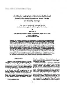
While implicit algebraic representations are easy to formulate, parametric surface representations are more complex and saw continuous evolution since the early seventies. Initially they were formed using power basis functions, which were not easy for CAD representations. Later, Bezier curves and surfaces [16] were introduced with the concept of having an approximating polygon that gives the rough shape of the free form curve. The actual curve is then formed by multiplying the control points on the polygon, which is better known as the control polygon, by some basis functions based on Bernstein polynomials (Figure 2.1).
Bezier curves and surfaces have two major drawbacks:
10 1. They do not offer some form of local control on curve segments (or surface patches) and hence do not provide the maximum flexibility, and 2. The degree of the curves increases with the increase in the number of control points, and hence cannot be used to approximate semi-quadratic surfaces with a large number of control points.
The drawbacks of Bezier surfaces were taken care of when B-Spline curves and surfaces were used for curve and surface fitting in the early nineties [26] [27]. Similar to Bezier curves/surfaces, B-Spline curves/surfaces depend on control polygons/nets to represent the approximate shape of the free form curves/surfaces. Their basis functions are piecewise polynomials defined between breakpoints (known as knot values) along the span of the independent parameters. Such definition over local spans of the independent parameters gives B-Splines a local modification property. In addition, the curve/surface degree is controllable. Control Polygon
3 2 1 0 -1 -6
-4
-2
0
2
4
6
Figure (2.1) Control polygon of free form curve
11 The advantages of B-Spline surfaces led to the fitting of surfaces that were too complex for previous representations such as swept surfaces [36]]. The problem of curve and surface fitting using B-Splines was addressed by Kitson [11].
A more general form of B-Spline curve/surfaces known as Non-Uniform Rational BSplines (NURBS) were used later for representing free form shapes [17]. Although NURBS are more general than mere B-Splines and give the maximum possible flexibility to the fitted curve/surface, their complex equations were not easy to use for surface fitting. Some recent publications [31] [32] and [28] use B-Splines in their initial fit then revert to NURBS for subsequent re-fitting.
2.3.2 Choice of Independent Parameters The fitting curves/surfaces have a multitude of independent parameters that can be used as independent variables for the minimization of the error function (Equation 2.1). Although the best solution to the error minimization problem would involve all independent variables, such choice might yield a large search space for the optimization algorithm. Therefore, reverse engineering researchers resort to the selection of some specific parameters as independent variables.
In the case of fitting implicit algebraic curves/surfaces, the curve/surface coefficients become the independent variables. Such curves/surfaces do not need any reduction in the number of independent variables since they are not as complex as free-form
12 representations. The estimation of such coefficients for different standard shapes is given thoroughly by Werghi et. al. [30].
B-Spline (or NURBS) curves/surfaces have the following parameters that need to be estimated either by some rough approximation or by their inclusion within the independent variables of the error minimization problem. 1. Control Points 2. Knot values 3. Weights (in case of NURBS surfaces) Piegl [17] made some approximate estimation of the knot values and optimized the values of the points. Huang et. al. [9] have Simulated various facial expression in animation by fixing the control points and changing weights, while Prahasto et. al. [19] optimized the knot vector for mult-curve B-Spline approximation.
The key to using a spline is the determination of good knots [23] [3]. In order to obtain a good curve or surface approximation, knots have to be placed as precisely as possible. A new alternative is presented by Yoo et. al. [34], which computes control points for approximation using object-oriented paradigm. This paradigm requires a central constructor evaluator, for generating the control points and derivatives for a given mapping. Computing control points is a classical approximation. Following the object oriented design principles of data hiding, the defining curves (private) control points are only accessed by their homogeneous evaluators and the approximation procedures does
13 not know about the ruling curves. A theoretically optimal solution for this is produced by meta-algorithm[18].
However, almost all of the more recent publications use a subset of the above parameters as independent variables. By adjusting the positions of control points and manipulating associated weights, one can design a large variety of shapes using NURBS. A matrix representation for NURBS curves and surfaces has been described by Gregory et. al. [6]. They represent the matrix form for NURBS by straightforward algebraic manipulation by using Bohem’s knot insertion algorithm instead of Deboor. For a NURB curve of degree ‘d’, the basic handles are control points, weights and knots. The method first performs a
linear transformation between t (knots) and u[0,1] by using a normalized parameter.
Usually subsets of the NURBS parameters are used as independent variables for optimization. The optimization of the control points and then the subsequent knot values was explored by Limeaiem et.al. [12] and Sarkar et. al. [26]. Raza [22] optimized both the knots and the weights corresponding to the control points for curve and surface fitting. Yau et. al. [32], then Shalaby et. al. [28] demonstrated that better flexibility of the fitted curve, and hence lower fitting errors, can be obtained by optimizing over the control points and then the weights of a NURBS curve/surface.
In [25], a simple tool addresses the problem of selecting the parameters of NURBS. It consists of a perspective functional transformation of arbitrary origin O. The extra
14 freedom provided by the weights in rational form is controlled in a geometric way without any numerical input. The displacement of several control points, keeping a common center O, can manipulate NURBS in ways that are simply impossible to achieve in integral form. This tool effectively employs the added flexibility provided by weights. By varying weights, a push/pull in the curve towards/away from the control points is created. Cases involving several control points in perspective functional transformations are also considered.
However, all of the previous fitting research resorted to a two-step approach, where the control points are estimated using least-squares approximation (which is the simplest form of quadratic programming) and then knots or weights are optimized using non-linear programming. The combination of subsets of the above parameters in the optimization problem has always been avoided on grounds of narrowing down the optimization search space, but in fact such combination still has to be explored.
2.3.3 Optimization Methods Used in Curve and Surface Fitting As mentioned in the above sub-section, the control points of a B-Spline/NURBS representation of a fitted curve/surface have been traditionally estimated using least squares. The knot values are either taken to be uniform or approximated according to the distribution of the measured points [17] and the weights are set to unity. After the estimation of the control points, optimizing over either the knot values or the weights further enhances the fitting. This enhancement is usually solved as a non-linear
15 programming problem. Gradient-based methods, such as Levenberg-Marquardt method [21], have been used for knot value optimization [26]. Direct search methods, such as Powell method, have also been used for the weights optimization [32]. Both approaches have the advantage of rapid convergence, but on the other hand may linger in local minima.
Yoshimoto et al.[33] proposed a new method that determines the number of knots and their locations simultaneously and automatically by using a G.A. This has the same problem of enlarged searched space. Raza [22] optimized both the knots and the weights corresponding to the control points using G.A's. The chromosomes have been constructed by considering the candidates of the locations of knots as genes.
Limeaiem et.al. [12] showed that the error minimization of parametric curves/surfaces is a global optimization problem, and used binary-coded GA’s [5] for knot values optimization. Although the binary-coded GA’s arrive to near global optimum solutions, the binary representation of the independent variables tend to enlarge the search space.
Shalaby et. al. [28] used real-coded GA’s for the optimization of the NURBS weights. Real-coded GA’s [37] have been proven to be better suited for continuous domain optimization. The same method has also been used by Nassef et. al. [15] for the fitting of prismatic features. However, both types of GA’s need a large number of objective
16 function evaluations and hence can be used only for fitting small curve/surface patches or prismatic features.
In [13], a general framework is setup for the application of genetic algorithms in curve design. Then, within this scheme, the problem of spline interpolation- a frequently used method for representing complex geometrical shapes in CAD/CAM system- is dealt with. While the method is simple and robust, it suffers from the drawback that some parameters must be given that are needed for the mathematical description but are not closely related to the geometrical input data of the object.
There are two other possible candidate global optimization methods that have not been used yet in surface fitting. These are: (1) Simulated Annealing (SA) and Tabu Search (TS). A good review of these methods is given by Pham et. al. [38]. Regarding the number of objective function evaluations, TS has the same drawback as GA’s, since it needs an excessive amount of objective function evaluations. This leaves SA as the candidate method to be explored for achieving globally minimum fitting errors with lower objective function evaluations.
A modified Tabu Search (T.S) global optimization technique has been used by Youssef [35], to optimize NURBS’ weights to minimize the fitting error in surface fitting, but a clear stopping criterion has not been used for this modified Tabu Search algorithm. To
17 our knowledge, the S.A. global optimization heuristic has not been applied to optimize NURBS parameters.
18
3 FITTING OF FREE-FORM SURFACES 3.1 Introduction As previously discussed in Chapter 2, the measured points obtained by the measuring devices are to be fitted into a surface in order to obtain the geometric model of the required object. The error function between the measured points and the fitted surface is given in equation 2.1. Minimization of this error function is the main problem to be solved. This chapter describes the surface representation used for the fitting operation and the steps performed in order to obtain the initial fit. In addition, the choice of the parameters that can be used as independent variables for the minimization of the error function is discussed in details.
3.2 Curve and Surface Basics 3.2.1 Implicit and Parametric Forms There are two main methods of representing curves and surfaces in geometric modeling. These methods are implicit equations and parametric functions.The implicit equation of a curve lying in the xy plane has the form f ( x, y ) = 0 . Figure 3.1 shows an example of the circle with unit radius centered at the origin, specified by the equation f ( x, y ) = x 2 + y 2 − 1 = 0 .
18
19 In parametric form, each of the coordinates of a point on the curve is represented separately as an explicit function of an independent parameter: C (u ) = ( x(u ), y (u ))
a≤u≤b
(3.1)
Therefore, C(u ) is a vector-valued function of the independent variable, u . Although the interval [a, b] is arbitrary, it is usually normalized to [0,1] . The circle shown in figure 3.1 is defined by the parametric functions: x(u ) = cos(u ) y (u ) = sin(u )
0≤u≤
π
(3.2)
2
Figure (3.1). A circle of radius 1, centered at the origin.
Surfaces can be defined by implicit equations of the form f ( x, y, z ) = 0 . For example the sphere of unit radius centered at the origin, shown in figure 3.2, can be specified by the equation x 2 + y 2 + z 2 − 1 = 0 . A parametric representation of the same sphere is given by S ( x(u, v), y (u , v), z (u , v)) , where x(u, v) = sin(u ) cos(v) y (u, v) = sin(u ) sin(v) z (u, v) = cos(u )
0 ≤u ≤π 0 ≤ v ≤ 2π
,
(3.3)
20 Both implicit and parametric forms have their advantages and disadvantages. Successful geometric modeling is done using both techniques. Piegl [17] gives a comparison between both representations as follows: •
By adding a z coordinate, the parametric method is easily extended to represent arbitrary curves in three-dimensional space, C (u ) = ( x(u ), y (u ), z (u )) ; the implicit form only specifies curves in the xy (or xz or yz ) plane.
Figure (3.2). A sphere of radius 1, centered at the origin.
•
It is difficult to represent bounded curve segments (or surface patches) with the implicit form. However, boundedness is built into the parametric form through the bounds on the parameter interval. On the other hand, unbounded geometry (e.g., a simple straight line given by f ( x, y ) = ax + by + c = 0 ) is difficult to implement using parametric geometry.
•
Parametric curves possess a natural direction of traversal (from C (a ) to C (b) if a ≤ u ≤ b ); implicit curves do not. Hence, it is easy to generate ordered sequences of
21 points along a parametric curve. A similar statement holds for generating meshes of points on surfaces. •
The complexity of many geometric operations and manipulations depends greatly on the method of representation.
Two classic examples are: •
Computing a point on a curve or surface, which is difficult in the implicit form and
•
Determining if a given point is on the curve or surface, which is difficult in the parametric form.
Parametric representations are the most suitable forms for representing free-form surfaces. Since the main concern of the presented thesis is the fitting of free-form surfaces to a set of measured points, the rest of this chapter concentrates on free-form representations.
3.2.2 Bezier Curves One of the early parametric curve and surface representations that became widely used is the Bezier representation. An nth-degree Bezier curve is defined by: n
C (u ) = ∑ Bi ,n (u ) Pi i =0
0 ≤ u ≤1
(3.4)
The basis (blending) functions, { Bi ,n (u ) }, are the classical nth-degree Bernstein polynomials given by:
Bi ,n (u ) =
n! u i (1 − u ) n −i i!(n − i )!
(3.5)
22 The geometric coefficients of this form, { Pi }, are called control points. The control points form a linear approximation of the free-form curve as shown in figure 2.5. The polynomial given by equation 3.5 covers the whole range of the independent parameter u.
3.2.3 Rational Bezier Curves It is known from classical geometry that all conic curves, including circles, can be represented using rational functions, which are defined as the ratio of two polynomials. In fact, they are represented with rational functions of the form:
x(u ) =
X (u ) W (u )
y (u ) =
Y (u ) W (u )
(3.6)
where X (u ), Y (u ) , and W (u ) are polynomials, that is, each of the coordinate functions has the same denominator. Thus an nth-degree rational Bezier curve is defined by: n
C (u ) = ∑ Ri ,n (u ) Pi i =0
where
Ri ,n (u ) =
Bi ,n (u ) wi n
∑ B j ,n (u ) w j
j =0
0 ≤ u ≤1
(3.7)
23 The Pi = (xi, yi, zi) represents control points and Bi,n (u) represents basis functions; the wi n
are scalars, called the weights. Thus, W (u ) = ∑ B j ,n (u ) wi is the common denominator j =0
function. It is assumed that wi > 0 for all i. This ensures that W (u ) > 0 for all u ∈ [0,1] .
3.2.4 Tensor Product Surfaces While a curve C (u ) is a vector-valued function of one parameter, a surface is a vectorvalued
function
of
two
parameters,
u
and
v.
Thus
it
has
the
form
S ( x(u, v), y (u , v), z (u , v)) , (u, v) ∈ R . There are many schemes for representing surfaces. Probably the simplest method, and the one most widely used in geometric modeling applications, is the tensor product scheme.
The tensor product method is basically a bi-directional curve scheme. It uses basis functions and geometric coefficients. The basis functions are bivariate functions of u and
v. Nonrational Bezier surfaces are obtained by taking a bi-directional net of control points and products of the univariate Bernstein polynomials:
S (u, v) = ∑ ∑ Bi ,n (u ) B j ,m (v )Pi , j n
m
i =0 j = o
0 ≤ u, v ≤ 1
(3.8)
A rational Bezier surface is defined as follows: n
m
S (u, v) = ∑ ∑ Ri , j (u, v) Pi , j i =0 j = o
where
0 ≤ u, v ≤ 1
(3.9)
24
Ri , j (u , v) =
Bi ,n (u ) B j ,m (v )wi , j ∑ ∑ Br ,n (u ) Bs ,m (v )wr ,s n
m
r =0 s = 0
Bezier curves and surfaces are considered to be a prelude to the more flexible B-Spline curves and surfaces.
3.3 B-Spline Curves and Surfaces 3.3.1 Definition and Properties of B-Spline Basis Functions Curves consisting of just one polynomial or rational segment (as in the case of Bezier curves) are often inadequate. Their shortcomings are: •
A high degree is required in order to satisfy a large number of constraints; e.g., ( n − 1 )-degree is needed to pass a polynomial Bezier curve through n data points. However, high degree curves are inefficient to process and are numerically unstable.
•
A high degree is required to accurately fit some complex shapes.
•
A change in one control point changes the whole curve and hence, there is no local control on segments of the curve.
The solution is to use curves (surfaces) which are piecewise polynomial, or piecewise rational of which the most common type is the B-Spline curves (surfaces). B-Spline curves use the same structure of Bezier curves, but the Bernstein polynomial (equation 3.5) is replaced with B-Spline basis function.
25 The following paragraph describes how a B-Spline curve is defined. Let U = {u 0 ,..., u m } be a non-decreasing sequence of real numbers, i.e., ui ≤ ui +1 , i = 0,..., m − 1 . The ui are called knots, and U is the knot vector. The ith B-Spline basis function of p-degree (order k), denoted by N i, p (u) , is defined as follows: N i ,0 (u ) = 1
if ui ≤ u < ui +1
N i ,0 (u ) = 0
otherwise
N i , p (u ) =
u i + p +1 − u u − ui N i +1, p −1 (u ) N i , p −1 (u ) + u i + p + 1 − u i +1 ui+ p − ui
(3.10)
Note that: •
N i ,0 (u ) is a step function, equal to zero everywhere except on the half-open interval u ∈ [ui , ui +1 ) .
•
For p > 0 , N i , p (u ) is a linear combination of two (p-1) -degree basis functions.
•
Computation of a set of basis functions requires specification of a knot vector, U, and the degree, p.
•
The N i , p is a piecewise polynomial, defined on the entire real line. Generally the interval [ui , u m ] is of interest.
•
The half-open interval, [ui , ui +1 ) , is called the ith knot span. It can have zero length, since knots need not be distinct.
26 Ex 3.1: Let U = {u 0 = 0, u1 = 0, u 2 = 0, u 3 = 1, u 4 = 2, u 5 = 3, u 6 = 4,
u 7 = 4, u8 = 5, u 7 = 4, u8 = 5, u 9 = 5, u10 = 5} and p = 2 . The zeroth-, first-, and seconddegree basis functions, which are not identically zero, are shown in figures 3.3, 3.4, and 3.5, respectively. B-Spline basis functions possess the following important properties : •
N i , p (u ) if u is outside the interval [ui , ui + p +1 ) (local support property).
•
In any given knot span, [u j , u j +1 ) , at most p + 1 i.e. k of the N i , p (u ) are nonzero, namely the functions N j − p , p ,..., N j , p .
•
N i , p (u ) for all i, p , and u (nonnegativity).
•
For an arbitrary knot span, [ui , ui +1 ) , ∑ N j , p (u ) = 1 for all u ∈ [ui , ui +1 ) (partition of
i
j =i − p
unity). Except for the case p = 0 , N i , p (u ) attains exactly one maximum value. Once the degree is fixed the knot vector completely determines the functions N i , p (u ) . There are several types of knot vectors. In this thesis, only nonperiodic (or clamped or open) knot vectors are considered. These have the form: U = {a,..., a, u p +1 ,..., u m− p −1 , b,..., b}
(3.11)
where there are p + 1 a’s and p + 1 b’s. That is the first and last knots have multiplicity p + 1 . The knots {u p +1 ,..., u m− p −1} are called interior knots. A knot vector U = {u 0 ,..., u m }
27 is defined to be uniform if all the interior knots are equally spaced; otherwise it is nonuniform.
Figure (3.3) The Non-Zero Zeroth-Degree Basis Functions, U = {0,0,0,1,2,3,4,4,5,5,5} .
Figure (3.4) The nonzero first-degree basis functions, U = {0,0,0,1,2,3,4,4,5,5,5} .(Youssef [35])
Figure (3.5).The nonzero second-degree basis functions, U = {0,0,0,1,2,3,4,4,5,5,5} .(Youssef [35])
3.3.2 Definition and Properties of B-Spline Curves A pth-degree B-Spline curve is defined by:
28 n
C (u ) = ∑ N i , p (u ) Pi i =0
(3.12)
where the {Pi } are the control points, and the {N i , p (u )} are the pth-degree B-Spline basis functions defined on the nonperiodic (and nonuniform) knot vector: U = {a,..., a, u p +1 ,..., u m− p −1 , b,..., b} . Generally, it is assumed that a = 0 and b = 1 . The polygon formed by the {Pi } is called the control polygon. Three steps are required to compute a point on a B-Spline curve at a fixed u value: 1. Find the knot span in which u lies. 2. Compute the nonzero basis functions. 3. Multiply the values of the nonzero basis functions with the corresponding control points. Examples of B-Spline curves (in some cases together with their basis functions) are shown in figures 3.6 through 3.14). B-Spline curves have the following properties: •
If n = p and U = {0,...,0,1,...,1} , where there are p+1 number of 0’s and p+1 number of 1’s, then C (u ) is a Bezier curve as shown in figure 3.6.
Figure (3.6) A cubic B-Spline curve on U = {0,0,0,0,1,1,1,1} , i.e., a cubic Bezier curve. (Youssef [35])
29 •
C (u ) is a piecewise polynomial curve (since the N i , p (u) are piecewise polynomials); the degree, p, number of control points, n + 1 , and number of knots, m + 1 , are related by: m = n + p +1
(3.13)
Figures 3.7 and 3.8 show basis functions and sections of the B-Spline curves corresponding to the individual knot span; in both figures the alternating solid/dashed segments corresponds to the different polynomials (knot spans) defining the curve. •
End point interpolation: C (0 ) = P0 and C (1) = Pn .
•
Affine invariance: an affine transformation is applied to the curve by applying it to the control points. Affine transformations include translations, rotations, scaling, and shears.
•
Strong convex hull property: the curve is contained in the convex hull of its control polygon; in fact, if u ∈ [ui , ui +1 ) , p ≤ i ≤ m − p − 1 , then C (u ) is in the convex hull of the control points Pi − p ,..., Pi (figures 3.9, 3.10, and 3.11). This follows from the nonnegativity and partition of unity properties of the N i , p (u ) , and the property that N i , p (u ) = 0 for u ∉ [ui , ui + p +1 ) . Figure 3.11 shows how to construct a quadratic curve containing a straight line segment. Since P2 , P3 , and P4 are colinear, the strong convex hull property forces the curve to be a straight line segment from C (2 / 5) to C (3 / 5) .
30
Figure (3.7a) Cubic basis functions on U = {0,0,0,0,1 / 4,1 / 2,3 / 4,1,1,1,1} .(Youssef [35])
Figure (3.7b) A cubic curve using the basis functions of figure 3.7a. (Youssef [35])
Figure (3.8a) Quadratic basis functions on U = {0,0,0,1 / 5,2 / 5,3 / 5,4 / 5,1,1,1} .(Youssef [35])
Figure (3.8b) A quadratic curve using the basis functions of figure 3.8a. (Youssef [35])
31
Figure (3.9) The strong convex hull property for a quadratic B-Spline curve; for u ∈ [u i , u i +1 ) , C (u ) is in the triangle Pi − 2 Pi −1 Pi .(Youssef [35])
Figure (3.10) The strong convex hull property for a cubic B-Spline curve; for u ∈ [u i , u i +1 ) ,
C (u ) is in the quadrilateral Pi −3 Pi − 2 Pi −1 Pi .(Youssef [35])
Figure (3.11) A quadratic B-Spline curve on U = {0,0,0,1 / 5,2 / 5,3 / 5,4 / 5,1,1,1} . The curve is a straight line between C ( 2 / 5) and C (3 / 5) .(Youssef [35])
32 •
Local modification scheme: moving Pi changes C (u ) only in the interval [ui , ui + p +1 ) (figure 3.12). This follows from the fact that N i , p (u ) = 0 for u ∉ [ui , ui + p +1 ) .
•
As a general rule, the lower the degree, the closer a B-Spline curve follows its control polygon (figures 3.13 and 3.14). The curves of figure 3.14 are defined using the same six control points, and the knot vectors:
p = 1 : U = {0,0,1 / 5,2 / 5,3 / 5,4 / 5,1,1} p = 2 : U = {0,0,0,1 / 4,1 / 2,3 / 4,1,1,1} p = 3 : U = {0,0,0,0,1 / 3,2 / 3,1,1,1,1} p = 4 : U = {0,0,0,0,0,1 / 2,1,1,1,1,1} p = 5 : U = {0,0,0,0,0,0,1,1,1,1,1,1} The reason for this phenomenon is intuitive: the lower the degree, the fewer the control points that are contributing to the computation of C (u0 ) for any given u 0 . The extreme case is p = 1 for which every point C (u ) is just a linear interpolation between two control points. In this case, the curve is the control polygon.
Figure (3.12) A cubic curve on U = {0,0,0,0,1 / 4,1 / 2,3 / 4,1,1,1,1} ; moving P4 (to P4 ) /
changes the curve in the interval [1 / 4,1) .(Youssef [35])
33 •
Moving along the curve from u = 0 to u = 1 , the N i , p (u ) functions act like switches; as u moves past a knot, one N i , p (u ) (and hence the corresponding Pi ) switches off, and the next one switches on (Figure 3.7 and 3.8).
3.3.3 Definition and Properties of B-Spline Surfaces A B-Spline surface is obtained by taking a bi-directional net of control points, two set of knot vectors, and the products of the univariate B-Spline functions: n
m
S (u, v) = ∑ ∑ N i , p (u ) N j ,q (v) Pi , j i =0 j =0
(3.14)
with U = {0,...,0, u p +1 ,..., u r − p −1 ,1,...,1} V = {0,...,0, vq +1 ,..., vs −q −1 ,1,...,1} where we have p + 1 of 0’s and p + 1 of 1’s in both U and V. U has r + 1 knots, and V has s + 1 , where r = n + p + 1 and s = m + q + 1
(3.15)
igure (3.13) B-Spline curves (a) A ninth-degree Bezier curve on the knot vector U = {0,0,0,0,0,0,0,0,0,0,1,1,1,1,1,1,1,1,1,1} .(Youssef [35])
34
Figure (3.13) B-Spline curves (b) A quadratic curve using the same control polygon defined on U = {0,0,0,1 / 8,2 / 8,3 / 8,4 / 8,5 / 8,6 / 8,7 / 8,1,1,1} .(Youssef [35])
Figure (3.14) B-Spline curves of different degrees, using the same control polygon. (Youssef [35])
Five steps are required to compute a point on a B-Spline surface at fixed (u, v) parameter values: 1. Find the knot span in which u lies, say u ∈ [ui , ui +1 ) . 2. Compute the nonzero basis functions N i − p , p (u ),..., N i , p (u ) . 3. Find the knot span in which v lies, say v ∈ [v j , v j +1 ) . 4. Compute the nonzero basis functions N j − q ,q (v),..., N j ,q (v) .
35 5. Multiply the values of the nonzero basis functions with the corresponding control points. Figures (3.15a and 3.15b) show the tensor product basis functions N 4 ,3 (u ) N 4 , 2 (v) and N 4 ,3 (u ) N 2 , 2 (v) respectively. Figures 3.16 to 3.19 show examples of B-Spline surfaces.
Figure (3.15) Product of a cubic and a quadratic basis function (a) N 4 , 3 (u )N 4 , 2 (v ) ;
U = {0,0,0,0,1 / 4,2 / 4,3 / 4,1,1,1,1} and V = {0,0,0,1 / 5,2 / 5,3 / 5,3 / 5,4 / 5,1,1,1} (Youssef [35]).
Figure (3.15) Product of a cubic and a quadratic basis function (b) N 4 , 3 (u )N 2 , 2 (v ) ;
U = {0,0,0,0,1 / 4,2 / 4,3 / 4,1,1,1,1} and V = {0,0,0,1 / 5,2 / 5,3 / 5,3 / 5,4 / 5,1,1,1} (Youssef [35]).
36 The properties of the tensor product basis functions follow from the corresponding properties of the univariate basis functions as follows: •
Nonnegativity: N i , p (u ) N j ,q (v) ≥ 0 for all i, j , p, q, u , v .
•
Partition of unity: ∑ ∑ N i , p (u ) N j ,q (v) = 1 for all (u , v) ∈ [0,1] × [0,1] . n
m
i = 0 j =0
•
If
n= p,
m=q,
U = {0,...,0,1,...,1} ,
and
V = {0,...,0,1,...,1} ,
then
N i , p (u ) N j ,q (v) = Bi ,n (u ) B j ,m (v) for all i, j ; that is, products of B-Spline functions degenerate to products of Bernstein polynomials. •
N i , p (u ) N j ,q (v) = 0 if (u, v) is outside the rectangle [ui , ui + p +1 ) × [v j , v j + q +1 ) (Figures 3.15a and 3.15b).
•
In any given rectangle, [ui0 , ui0 +1 ) × [v j0 , v j0 +1 ) , at most ( p + 1)(q + 1) basis functions are nonzero, in particular the N i , p (u ) N j ,q (v) for i0 − p ≤ i ≤ i0 and j0 − q ≤ j ≤ j0 .
•
If p > 0 and q > 0 , then N i , p (u ) N j ,q (v) attains exactly one maximum value (figures 3.15a and 3.15b).
B-Spline surfaces have the following properties: •
If n = p , m = q , U = {0,...,0,1,...,1} , and V = {0,...,0,1,...,1} , then S (u, v) is a Bezier surface.
•
The surface interpolates the four corner control points: S (0,0 ) = P0 ,0 , S (1,0) = Pn ,0 , S (0,1) = P0 ,m , and S (1,1, ) = Pn ,m (figures 3.16 through 3.19).
37
Figure (3.16a) A B-Spline surface-control net (Youssef [35]).
Figure (3.16b) A B-Spline surface (Youssef [35]). •
Affine invariance: an affine transformation is applied to the surface by applying it to the control points.
•
Strong convex hull property: if (u, v) ∈ [u i0 , u i0 +1 ) × [v j0 , v j0 +1 ) , then S (u, v) is in the convex hull of the control points Pi , j , i0 − p ≤ i ≤ i0 and j0 − q ≤ j ≤ j0 (figure 3.17).
38
Figure (3.17a) Product of a cubic and a quadratic B-Spline surface (Youssef [35]).
Figure (3.17b) The strong convex hull property (Youssef [35]).
39 •
If triangulated, the control net forms a piecewise planar approximation to the surface; as is the case for curves, the lower the degree the better the approximation (figures 3.18a and 3.18b).
Figure (3.18a) A biquadratic surface (Youssef [35]).
Figure (3.18b) A biquadratic surface (p = q = 4 ) using figure 3.18a control points (Youssef [35]).
40 •
Local modification scheme: if Pi , j is moved, it affects the surface only in the rectangle [ui , ui + p +1 ) × [v j , v j + q +1 ) . Now consider figures 3.19a and 3.19b: the initial surface is flat because all the control points lie in a common plane; the control net is offset from the surface only for better visualization. When P3,5 is moved, it affects the surface shape only in the rectangle [1 / 4,1) × [2 / 5,1) .
Figure (3.19a) A product of a planar quadratic and a cubic surface,
U = {0,0,0,1 / 4,1 / 2,3 / 4,1,1,1} and V = {0,0,0,0,1 / 5,2 / 5,3 / 5,4 / 5,1,1,1,1} (Youssef [35]).
Figure (3.19b) P3,5 is moved, affecting surface shape only in the rectangle [1 / 4,1) × [ 2 / 5,1) (Youssef [35]).
41
3.4 Rational B-Spline Curves and Surfaces 3.4.1 Definition and Properties of Non-Uniform Rational B-Spline Curves A Non-Uniform Rational B-Spline Curve, denoted by NURBS, of degree p is defined by: n
C (u ) = ∑ Ri , p (u ) Pi
a≤u≤b
i =0
(3.16)
where Ri , p (u ) =
N i , p (u ) wi
(3.17)
n
∑ N j , p (u ) w j
j =0
where {Pi } are the control points (forming a control polygon), {wi } is the set of weights, the {N i , p (u )} is the set of pth-degree B-Spline basis functions defined on the nonperiodic (and nonuniform) knot vector: U = {a,..., a, u p +1 ,..., u m− p −1 , b,..., b} {Ri , p (u )} is the set of rational basis functions; they are piecewise rational functions on u ∈ [0,1] where we assume that a = 0 , b = 1 , and wi > 0 for all i.
Ri , p (u ) have the following properties: •
Nonnegativity: Ri , p (u ) ≥ 0 for all i, p , and u ∈ [0,1] .
•
Partition of unity: ∑ Ri , p (u ) = 1 for all u ∈ [0,1] . n
i =0
42 •
R0 , p (0) = Rn , p (1) = 1 .
•
For p > 0 , all Ri , p (u ) attain exactly one maximum value on the interval u ∈ [0,1] .
•
Local support: Ri , p (u ) = 0 for u ∉ [ui , ui + p +1 ) . Furthermore, in any given knot span, at most p + 1 i.e. k (order of the curve) of the Ri , p (u ) are nonzero (in general, Ri − p , p (u ),..., Ri , p (u ) are nonzero in [ui , ui +1 ) ).
•
If wi = 0 for all i , then Ri , p (u ) = N i , p (u ) for all i ; i.e., N i , p (u ) is a special case of Ri , p (u ) . In fact, for any a ≠ 0 , if wi = a for all i then Ri , p (u ) = N i , p (u ) for all i .
•
The previous properties yield the following important geometric characteristics of NURBS curves:
•
Affine invariance: an affine transformation is applied to the curve by applying it to the control points; NURBS curves are also invariant under perspective projections, which is very important in computer graphics.
•
Strong convex hull property: if u ∈ [ui , ui +1 ) , then C (u ) lies within the convex hull of the control points Pi − p ,..., Pi (figure 3.20, where C (u ) for u ∈ [1 / 4,1 / 2) (dashed segment) is contained in the convex hull of {P1 , P2 , P3 , P4 } , the dashed area).
•
A NURBS curve with no interior knots is a rational Bezier curve, since the N i , p (u ) reduce to the Bi ,n (u ) . This implies that NURBS curves contain nonrational B-Spline and rational and nonrational Bezier curves as special cases.
43 •
Local approximation: if the control point Pi is moved, or the weight wi is changed, it affects only that portion of the curve on the interval u ∈ [ui , ui + p +1 ) .
Figure (3.20a) U = {0,0,0,0,1 / 4,1 / 2,3 / 4,1,1,1,1} and {w0 ,..., w6 } = {1,1,13,1,1,1} A cubic NURBS curve. (Youssef [35])
Figure (3.20b) U = {0,0,0,0,1 / 4,1 / 2,3 / 4,1,1,1,1} and {w0 ,..., w6 } = {1,1,13,1,1,1} Associated basis functions. (Youssef [35])
The last property is very important for refining surface fits to measured points. Using NURBS curves, both control point movement and weight modification can be utilized to attain local shape control. Figures 3.21 to 3.25 show the effects of modifying a single weight. (eg: Assuming u ∈ [ui , ui + p +1 ) , the effect is that if wi increases (decreases), the point Cu moves closer to (farther from) Pi , and hence the curve is pulled toward (pushed
44 away from) Pi . Furthermore, the movement of Cu for fixed u is along a straight line (figure 3.25)). In figure 3.25, u is fixed and w3 is changing. Let B = C (u; w3 = 0 ) and N = C (u; w3 = 1) . Then the straight line defined by B and N passes through P3 , and for arbitrary 0 < w3 < ∞ , B3 = C (u; w3 ) lies on this line segment between B and P3 .
Figure (3.21) Rational cubic B-Spline curves, with w3 varying. (Youssef [35])
Figure (3.22a) The cubic basis functions for the curves of figure 3.21 (Youssef [35])
Figure (3.22b) The cubic basis functions for the curves of figure 3.21(Youssef [35])
(b) w3 = 3 / 10 .
45
Figure (3.22c) The cubic basis functions for the curves of figure 3.21 (c) w3 = 0 .(Youssef
[35])
Figure (3.23) Rational quadratic curves, with w1 varying. (Youssef [35])
Figure (3.24a) The quadratic basis functions for the curves of figure 3.23 w1 = 4 .(Youssef [35])
46
Figure (3.24b) The quadratic basis functions for the curves of figure 3.23 w1 = 3 / 10 .(Youssef [35])
Figure (3.24c) The quadratic basis functions for the curves of figure 3.23 w1 = 0 .(Youssef [35])
Figure (3.25) Modification of the weight w3 .(Youssef [35])
47
3.4.2 Definition and Properties of NURBS Surfaces A NURBS surface of degree p in the u direction and degree q in the v direction is a bivariate vector-valued piecewise rational function of the form: n
m
S (u , v) = ∑ ∑ Ri , j (u ) Pi , j i =0 j = o
0 ≤ u, v ≤ 1
(3.18)
where Ri , j (u, v) =
N i , p (u ) N j ,q (v) wi , j n m
(3.19)
∑ ∑ N k , p (u ) N l , p (v) wk ,l
k =0 l = 0
{Pi , j } forms a bi-directional control net, {wi , j } is the set of weights, Ri , j (u, v) are the piecewise rational basis functions for 0 ≤ i ≤ n and 0 ≤ j ≤ m , and {N i , p (u )} and {N j ,q (v)} are the nonrational B-Spline basis functions defined on the knot vectors: U = {0,...,0, u p +1 ,..., u r − p −1 ,1,...,1} V = {0,...,0, vq +1 ,..., vs −q −1 ,1,...,1} where there are p + 1 0’s and p + 1 1’s and r = n + p + 1 and s = m + q + 1 Figures 3.26 and 3.27 show examples of NURBS surfaces.
48
Figure (3.26a ) Control net and biquadratic NURBS surface, w1,1 = w1, 2 = w2,1 = w2, 2 = 10 with the rest of the weights 1 . U = V = {0,0,0,1 / 3,2 / 3,1,1,1} Control net (Youssef [35]).
Figure (3.26b) Control net and biquadratic NURBS surface, w1,1 = w1, 2 = w2,1 = w2, 2 = 10 with the rest of the weights 1 . U = V = {0,0,0,1 / 3,2 / 3,1,1,1} Biquadratic NURBS surface (Youssef [35]).
49
Figure (3.27) Bicubic NURBS surface defined by the control net in figure 3.26a, with U = V = {0,0,0,0,1 / 2,1,1,1,1} and with the same weights (Youssef [35]).
The important properties of the functions Ri , j (u, v) are the same as those given in Section 3.3 for the nonrational basis functions,
N i , p (u ) N j ,q (v)
The following are the main properties of NURBS surfaces: •
Corner points interpolation: S (0,0 ) = P0 ,0 , S (1,0) = Pn ,0 , S (0,1) = P0 ,m , S (1,1) = Pn , m .
•
Affine invariance: an affine transformation is applied to the surface by applying it to the control points.
•
Strong
convex
hull
property:
assume
wi , j ≥ 0
for
all
i, j .
If
(u , v) ∈ [u i 0 , u i 0 +1 ) × [ v j0 , v j0 +1 ) , then S (u, v) is in the convex hull of the control points Pi , j , i0 − p ≤ i ≤ i0 and j0 − q ≤ j ≤ j0 . •
Local modification: if Pi , j is moved, or wi , j is changed, it affects the surface shape only in the rectangle [ui , ui + p +1 ) × [vi , v j + q +1 ) .
50 •
Nonrational B-Spline and Bezier and rational Bezier surfaces are special cases of NURBS surfaces. It is obvious that both control point movement and weight modification to locally change the shape of NURBS surfaces. Figures 3.28a and 3.28b show the effects on the basis function Ri , j (u, v) and the surface shape when a single weight, wi , j , is modified. (eg: Assuming (u, v) ∈ [u i , u i + p +1 ) × [v j , v j + q +1 ) , then the effect on the surface if wi , j increases (decreases), the point S (u, v) moves closer to (farther from) Pi , j and hence the surface is pulled toward (pushed away from) Pi , j ).
Figure (3.28a) The basis function R4 , 2 (u , v ) , with U = {0,0,0,0,1 / 4,1 / 2,3 / 4,1,1,1,1} and
V = {0,0,0,1 / 5,2 / 5,3 / 5,3 / 5,4 / 5,1,1,1} , wi , j = 1 for all (i, j) ≠ (4,2) (Youssef [35]).
51
Figure (3.28b) The basis function R4 , 2 (u , v ) , with U = {0,0,0,0,1 / 4,1 / 2,3 / 4,1,1,1,1} and
V = {0,0,0,1 / 5,2 / 5,3 / 5,3 / 5,4 / 5,1,1,1} , wi , j = 1 for all (i, j) ≠ (4,2) (Youssef [35]).
3.5 Curve and Surface Fitting This section describes the fitting of free-form curves and surfaces to an arbitrary set of geometric data, such as points and derivative vectors. Two types of fitting are distinguished : interpolation and approximation. In interpolation, the constructed curve or surface satisfies the given points precisely, e.g., the curve passes through the given points and assumes the given derivatives at the prescribed points. Figure 3.29 shows a curve interpolating five points and the first derivative vectors at the endpoints.
Figure (3.29) A curve interpolating five points and two end derivatives.
52 In approximation, the constructed curves and surfaces do not necessarily satisfy the given data precisely, but only approximately. In some applications, an example is generation of point data by use of coordinate measuring devices or digitizing tablets. In this case it is important for the curve or surface or surface to capture the “shape” of the data, but not to “wiggle” its way through every point. In approximation, it is often desirable to specify a maximum bound on the derivation of the curve or surface from the given data, and to specify certain constraints.
Figure 3.30 shows a curve approximating a set of m+1 points. A maximum deviation bound, E, was specified, and the perpendicular distance, ei, is the approximation error obtained by projecting Qi on the curve. The ei of each point, Qi, is less than E. The end point Qo and Qm were specified as constraints, with the result that eo = em = 0. Input to a fitting problem generally consists of geometric data, such as points or derivatives. Output is a curve or surface, after the calculation of control points and knots. Furthermore, either the degree p (or (p, q) for surfaces) must be input.
Figure (3.30) A curve approximating m+1 points; the curve is constrained to pass through the end points, Q0 and Qm.
53
3.6 Optimization of NURBS Parameters The evaluation of the control points by least squares approximation can be viewed as an initial estimation of the fitted surface. Further refinement can be obtained by optimizing the different NURBS parameters, such as the knot values and the weights in order to achieve better fitting accuracy. The error function between the measured points and the fitted surface is generally given by equation (2.1). This equation has been specified to suit the NURBS representation of the fitted surface as follows: ⎛ s E = ⎜ ∑ Qk − Qek ⎝ k =0
r
⎞ s⎟ ⎠
1/ r
(3.41)
where: 1. Qk is the kth-measured point. 2. Qek is the equivalent point on the surface to the kth-measured point. Accurately, this point would be found by orthogonally projecting the measured point on the fitted surface. Such evaluation would lead to cumbersome computations and hence in Dierckx [3], this point is approximated by P (u k , v l ) , where u k and v l are the independent parameters associated with measured point Qk . 3. r is the exponent. If the average deviation is to be minimized, then r is set to either 1 or 2 (least-squares deviation function). Setting r to infinity leads to the minimization of the maximum deviation. The selection of such exponent depends on the measurement device and its accuracy [15]. For the problem in hand the measurement device is a laser scanner so the value used for r is 2.
54 4. s is the number of measured points.
Shalaby et.al. [28] showed that better results could be obtained by optimizing the weights while keeping the knot values uniformly distributed. The fitting task can be viewed mathematically as an approximation problem between an unknown function, represented by a set of measured points {Q}, and an approximating function, represented by the geometric model of the fitted curve/surface S(α1, ...., αn), where {α1, ...., αn} are the parameters of the fitted curve/surface. The general formulation of the objective function of the optimization problem is represented by the following equation: ⎞ ⎛ s r E = ⎜ ∑ Qi − S (α 1 ,..., α n ) s ⎟ ⎠ ⎝ i =0
1/ r
(3.42)
where s is the number of measured points, and r is an exponent, ranging from 1 to infinity. The fitting task can then be viewed as the optimization of the curve/surface parameters {α 1 ,..., α n } to minimize the error E
However the weights present a large number of independent variables (equaling the number of control points) to the optimization problem, which may lead to a large search space. In addition, the fitting of free-form surfaces to the measured points has been shown by Shalaby et. al.
[28] as well as by Limeaiem et.al. [12] to be a multi-modal
optimization problem. Therefore, global optimization techniques are needed for optimizing such problems. Other researchers have used different variants of Genetic Algorithms (GA’s), but all came to the conclusion that GA’s need a large number of
55 objective function evaluations. Since reverse engineering of free-form surfaces processes a large number of measured points, the single evaluation of the objective function is computationally exhaustive. The above findings inspired the research of the presented thesis to be focused on Simulated Annealing (SA). SA is one of the global optimization methods like GA’s and Tabu Search (TS). The next chapter presents an approach to the global optimization of continuous functions based on Simulated Annealing.
4 SIMULATED ANNEALING 4.1 Introduction Simulated Annealing (S.A.) exploits analogy between the way in which a metal cools and freezes into a minimum energy crystalline structure (the Annealing process) and the search for a minimum in a general system. If a physical system is melted and then cooled slowly, the entire system can be made to produce the most stable (crystalline) arrangement, and not get trapped in a local minimum.
The S.A. algorithm was first proposed by Metropolis et. al. [14] as a means to find equilibrium configuration of a collection of atoms at a given temperature. Kirkpatrick et. al. [10] were the first to use the connection between this algorithm and mathematical minimization as the basis of an optimization technique for combinatorial (as well as other) problems.
S.A’s major advantage over other methods is its ability to avoid being trapped in local minima. The algorithm employs a random search, which not only accepts changes that decrease the objective function E, but also some changes that would increase it. The latter are accepted with a probability
Prob(accept) = exp(-∆E/T)
56
57 where ∆E is the increase in E and T is a control parameter, which by analogy with the original application is known as the system “temperature” irrespective of the objective function involved.
Briefly S.A. works in the following way. Given a function to optimize, and some initial values for the variables, Simulated Annealing starts at a high, artificial, temperature. While cooling the temperature slowly, it repeatedly chooses a subset of the variables, and changes them randomly in a certain neighborhood of the current point. If the objective function has a lower function value at the new iterate, the new values are chosen to be the initial values for the next iteration. If the objective function has a higher function value at the new iterate, then the new values are chosen to be the initial values for the next iteration with a certain probability, depending on the change in the value of the objective function and the temperature.
The higher the temperature and the lower the change, the more probable that the new values are chosen to be the initial variables for the next iteration. Throughout this process, the temperature is decreased gradually, until eventually the values do not change anymore. Then, the function is presumably at its global minimum. The global minimum is obtained by choosing an appropriate “cooling schedule” which includes the temperature and its cooling rate. A cooling schedule describes the temperature parameter T, and gives rules for lowering it as the search progresses.
58
4.2 Simulated Annealing Algorithm The Simulated Annealing algorithm is shown in Figure 4.1(a) and the Metropolis procedure used by the algorithm is shown in figure 4.1(b). Algorithm Simulated_Annealing (So, To, α, β, M, Maxtime); (*So is the initial solution *) (*BestS is the best solution*) (*To is the initial temperature*) (*α is the cooling rate*) (*β a constant*) (*Maxtime is the total allowed time for the Annealing process*) (*M represents the time until the next parameter update*) Begin T = To; CurS = So; BestS = CurS;
/*BestS is the best solution seen so far */
CurCost = Cost(CurS); BestCost = Cost(BestS); Time = 0; Repeat Call Metropolis(CurS, CurCost, BestS, BestCost, T, M ); Time = Time + M; T = α T; M = β M; Until (Time ≥ MaxTime); Return (BestS) End (* of Simulated Annealing *) Figure (4.1a) The Simulated Annealing Algorithm.
59 Algorithm Metropolis(CurS, CurCost, BestS, BestCost, T, M ); Begin Repeat NewS = Neighbor(CurS); NewCost = Cost(NewS);
∆Cost = (NewCost – CurCost); If (∆Cost < 0) Then CurS = NewS; If NewCost < BestCost Then BestS = NewS EndIf Else If (RANDOM < e-∆Cost/T) Then CurS = NewS; EndIf EndIf M=M–1 Until (M = 0) End (*of Metropolis*) Figure (4.1b) The Metropolis procedure.
The Metropolis procedure, which simulates the Annealing process at a given temperature T, is the core of the S.A algorithm. The Metropolis procedure receives as input the current temperature T, and the current solution CurS, which it improves through local search. Finally, Metropolis must also be provided with the value M, which is the amount of time for which Annealing must be applied for a temperature T.
60 The procedure Simulated_Annealing simply invokes Metropolis at decreasing temperatures. Temperature is initialized to a value To at the beginning of the procedure, and is reduced in a controlled manner (typically in a geometric progression); the parameter α is used to achieve this cooling. The amount of time spent in Annealing at a temperature is gradually increased as temperature is lowered. This is done using the parameter β > 1.The variable Time keeps track of the time being expended in each call to the Metropolis. The Annealing procedure halts when Time exceeds the allowed time.
The Metropolis procedure uses the procedure Neighbor to generate a local neighbor NewS of any given solution S. The function Cost returns the cost of a given solution S. If the cost of the new solution NewS is better than the cost of the current solution CurS, then the new solution is accepted, and we do so by setting CurS = NewS. If the cost of the new solution is better than the best solution (BestS) seen thus far, we replace BestS by NewS. If the new solution has a higher cost in comparison to the original solution CurS, Metropolis will accept the new solution on a probabilistic basis. A random number (RANDOM) is generated in the range 0 to 1. If this random number is smaller than e-∆Cost/T , where ∆Cost is the difference in costs, and T is the current temperature, the uphill solution is accepted. This criterion for accepting the new solution is known as the Metropolis criterion. The Metropolis procedure generates and examines M solutions.
The probability that an inferior solution is accepted by the Metropolis, is given by
61 P(RANDOM < e-∆Cost/T). The random number generation is assumed to follow a uniform distribution. Remember that ∆Cost > 0 since we have assumed that NewS is uphill from CurS. At very high temperatures, (when T → ∞), e-∆Cost/T ≈ 1. and hence the above probability approaches 1. On the contrary, when T → 0, the probability e-∆Cost/T falls to 0.
In order to implement Simulated Annealing, we need to formulate a suitable cost function for the problem being solved. In addition, as in the case of local search techniques, we assume the existence of a neighborhood structure, and need Neighbor function to generate new states (neighborhood states) from current states. And finally we need a cooling schedule that describes the temperature parameter T and gives rules for lowering it.
4.3 Parameters of the S.A. algorithm If S.A is allowed to run for an infinitely long time, starting with a high value of T, and allowing T Æ 0, then it will find a desired optimal configuration. In practice, however, Simulated Annealing is only run for a finite amount of time. A finite time implementation can be realized by generating homogeneous Markov chains of finite lengths for a sequence of decreasing values of temperature. T0 achieve this, a set of parameters that govern the convergence of the algorithm must be specified. This set of parameters is commonly referred to as the “cooling schedule”.
62 The Metropolis procedure receives as input the current temperature T, the current solution CurS, and a value M, which is the amount of time for which Annealing must be applied at temperature T. Temperature is initialized to a value T0 at the beginning of the procedure, and is slowly reduced in a geometric progression; the parameter α is used to achieve this cooling. The amount of time spent in Annealing at a given temperature is gradually increased as temperature is lowered. This is done using the parameter β ≥ 1. The variable Time keeps track of the time being expended in each call to the Metropolis. The Annealing procedure halts when Time exceeds the allowed time. The cooling schedule specifies the following: A finite sequence of values of temperature, which are given by the initial value T0 , a decrement factor (α), and the final value, which is specified by the stopping criterion. A finite number of transitions (denoted by βM) at each value of the temperature, which corresponds to the finite length of each homogeneous Markov chain.
Therefore, a cooling schedule is completely specified by setting the values of parameters α, β, M, T0 and Time. It is customary to determine the schedule by trial and error. However, some researches have proposed cooling schedules that rely on some mathematical rigor. In our work, we have used the cooling schedule presented by Kirkpatrick et al [Kirkpatrick 83].
63
4.4 S.A. Requirements In order to use Simulated Annealing to solve a particular problem, a sequence of Markov chains is to be generated at descending values of temperature. As seen earlier, the inner loop of the Annealing algorithm is a homogeneous Markov chain, and T does not change within the loop. Such Markov chains are generated by transforming a current solution to another one by applying a generation mechanism (perturbance or neighbor function) and using an acceptance function which is usually the Metropolis function. Application of the Annealing algorithm therefore requires the following.
1. A concise representation of the state space, where each state represents a configuration, and a cost function that represents the cost effectiveness of the solutions with respect to the optimization objectives. It is important that the solution representation be easy to manipulate. Furthermore, the cost function should be given by a simple expression that is easy to evaluate. This requirement is important because the manipulation of current configurations to generate new neighborhood states and the evaluation of the cost of that solution are done a large number of times. 2. A mechanism for transforming the current solution into a subsequent one to which the search should move. This will involve two steps. a. First, the neighbor function is applied to generate a new solution. T0 guarantees asymptotic convergence to the set of optimal solutions, the
64 neighborhood structure must be properly chosen so that the corresponding generation mechanism induces an irreducible and aperiodic Markov chain. b. Second, the cost of this new solution, and hence the difference in cost ∆Cost is computed. Then, a decision is made whether to accept or reject this newly generated solution. These two steps are the most time consuming and should be executed in a time efficient manner. Therefore, in practice, the neighbor functions are generally simple. 3. Finally, the success of a S.A algorithm depends on the choice of a proper cooling schedule, that is, on the initial value of temperature, the decrement function, the length of the Markov chain and a suitable stopping criterion.
5 THE PROPOSED METHOD 5.1 Introduction Figures 5.1a and 5.1b shows the basic building blocks of our implemented system for curves and surfaces respectively for weight optimization. We discuss Figure 5.1 briefly below.
Initially a character/surface is scanned to get a digitized image. In case of curves, its contour is extracted using boundary detection algorithms, to obtain a number of data points. We assume that the curves are continuous, i.e. they possess single segments. The parametric value ‘u’ for each data point is then calculated using chord length parameterization [24]. In the case of a surface, the parameter calculation is bi-directional. The least squares technique is used to calculate the control points. A uniform knot vector is calculated in the case of a curve and two uniform knot vectors are calculated in the case of a surface, in ‘u’ and ‘w’ directions. Then, Simulated Annealing is used to optimize weights. Once the values of all three space parameters – control points, knot vector and weights are received, the NURBS curve is fitted to obtain a geometric model of the curve.
65
66
5.2 Obtaining a digitized image/surface Figure 5.3 discusses in detail our proposed approach. A digitized image is obtained from an electronic device or by scanning an image. The quality of digitized scanned image depends of various factors such as the image on paper, scanner type and the attributes set during scanning. The quality of digitized image obtained directly from an electronic device depends on the resolution device, source of image, type of image, etc. Some of the digitized images/surfaces are shown in Figure 5.2. The surfaces are generated using mathematical functions. The Table 5.1shows the surfaces, with their respective generator functions. Table (5.1) Surface generating functions
Surfaces
Functions
Surface 1
R = ( x 2 + y 2 ; z = Sin( R) R
Surface 2 [X,Y,Z] = Cylinder( 2 + cos(t)) Surface 3
[X,Y,Z] = Sphere(N)
67
Figure (5.1a) Curve – weight optimization.
Figure (5.1b) Surface – weight optimization.
In Table 5.1, cylinder and sphere are the matlab functions which generate a cylinder and a sphere respectively, where ‘t’ is a parameter in surface 2 and N produces (N+1) by (N+1) matrices of X,Y & Z for surface 3.
68
5.3 Contour extraction The contour of the digitized image is extracted using the boundary detection algorithms. There are numerous algorithms for detecting boundary. We used the algorithm proposed by Quddus [20]. The input to this algorithm is a bitmap file. The algorithm returns a number of segments and for each segment, a number of boundary points and their values. Table 5.1 gives the number of boundary points detected by the boundary detection algorithm for the word ‘Ali’, the symbol ‘Pound’ and the letter ‘Aich’ and the number of points scanned for surfaces.
Table (5.2) Scanned data points
S.No Name of the Figure
# of data points
1
Ali
1640
2
Pound
689
3
Aich
320
4
Apple
1204
5
Open Curve
1001
4
Surface 1
1089
5
Surface 2
441
6
Surface 3
1024
7
Jar
1089
69 In case of surfaces, Table 5.1 shows their generating functions. Using these generating functions, input data points are generated for the surfaces. The Tables 5.3 to 5.6 show the data points generated for Surface1, Surface 2, Surface 3 & Jar respectively.
Aich
Ali
Apple
Surface 2
Open Curve
Surface3 Figure (5.2) Input Curves and Surfaces.
Pound
Surface1
Jar
70 Table(5.3) Sample data points for Surface 1 2.5 -7.5 0.126322 3 -7.5 0.12071 3.5 -7.5 0.1102 4 -7.5 0.0939397 4.5 -7.5 0.0717446 5 -7.5 0.0443133 5.5 -7.5 0.0133241 6 -7.5 -0.0186304 6.5 -7.5 -0.0483008 7 -7.5 -0.0722156 7.5 -7.5 -0.087238 8 -7.5 -0.0911519 -8 -7 -0.0878606 -7.5 -7 -0.0722156 -7 -7 -0.0461727 -6.5 -7 -0.0133328 -6 -7 0.0221048 -5.5 -7 0.0560617 -5 -7 0.0851882 -4.5 -7 0.107264 -4 -7 0.121354 -3.5 -7 0.127726 -3 -7 0.127599 -2.5 -7 0.12279 -2 -7 0.115356 -1.5 -7 0.10728 -1 -7 0.100248 -0.5 -7 0.0955176 0 -7 0.0938552 0.5 -7 0.0955176 1 -7 0.100248 1.5 -7 0.10728 2 -7 0.115356 2.5 -7 0.12279 3 -7 0.127599 3.5 -7 0.127726 4 -7 0.121354 4.5 -7 0.107264 5 -7 0.0851882 5.5 -7 0.0560617 6 -7 0.0221048 6.5 -7 -0.0133328 7 -7 -0.0461727 7.5 -7 -0.0722156 8 -7 -0.0878606 -8 -6.5 -0.0749569 -7.5 -6.5 -0.0483008 -7 -6.5 -0.0133328 -6.5 -6.5 0.0250537 -6 -6.5 0.0618459
-2 -6.5 0.0727498 -1.5 -6.5 0.0566662 -1 -6.5 0.0439599 -0.5 -6.5 0.0358682 0 -6.5 0.0330954 0.5 -6.5 0.0358682 1 -6.5 0.0439599 1.5 -6.5 0.0566662 2 -6.5 0.0727498 2.5 -6.5 0.090402 3 -6.5 0.10728 3.5 -6.5 0.120673 4 -6.5 0.127814 4.5 -6.5 0.126322 5 -6.5 0.114689 5.5 -6.5 0.0927286 6 -6.5 0.0618459 6.5 -6.5 0.0250537 7 -6.5 -0.0133328 7.5 -6.5 -0.0483008 8 -6.5 -0.0749569 -8 -6 -0.0544021 -7.5 -6 -0.0186304 -7 -6 0.0221048 -6.5 -6 0.0618459 -6 -6 0.0951366 -5.5 -6 0.117888 -5 -6 0.127914 -4.5 -6 0.125067 -4 -6 0.110992 -3.5 -6 0.0886112 -3 -6 0.0614677 -2.5 -6 0.0330954 -2 -6 0.00653931 -1.5 -6 -0.0159051 -1 -6 -0.0327292 -0.5 -6 -0.0430819 0 -6 -0.0465692 0.5 -6 -0.0430819 1 -6 -0.0327292 1.5 -6 -0.0159051 2 -6 0.00653931 2.5 -6 0.0330954 3 -6 0.0614677 3.5 -6 0.0886112 4 -6 0.110992 4.5 -6 0.125067 5 -6 0.127914 5.5 -6 0.117888 6 -6 0.0951366
5.5 -5 0.12279 6 -5 0.127914 6.5 -5 0.114689 7 -5 0.0851882 7.5 -5 0.0443133 8 -5 -0.00097552 -8 -4.5 0.0265312 -7.5 -4.5 0.0717446 -7 -4.5 0.107264 -6.5 -4.5 0.126322 -6 -4.5 0.125067 -5.5 -4.5 0.103188 -5 -4.5 0.063807 -4.5 -4.5 0.0126789 -4 -4.5 -0.0430819 -3.5 -4.5 -0.0964682 -3 -4.5 -0.141902 -2.5 -4.5 -0.176131 -2 -4.5 -0.198521 -1.5 -4.5 -0.210717 -1 -4.5 -0.215789 -0.5 -4.5 -0.217107 0 -4.5 -0.217229 0.5 -4.5 -0.217107 1 -4.5 -0.215789 1.5 -4.5 -0.210717 2 -4.5 -0.198521 2.5 -4.5 -0.176131 3 -4.5 -0.141902 3.5 -4.5 -0.0964682 4 -4.5 -0.0430819 4.5 -4.5 0.0126789 5 -4.5 0.063807 5.5 -4.5 0.103188 6 -4.5 0.125067 6.5 -4.5 0.126322 7 -4.5 0.107264 7.5 -4.5 0.0717446 8 -4.5 0.0265312 -8 -4 0.0516787 -7.5 -4 0.0939397 -7 -4 0.121354 -6.5 -4 0.127814 -6 -4 0.110992 -5.5 -4 0.0727498 -5 -4 0.0186864 -4.5 -4 -0.0430819 -4 -4 -0.103622 -3.5 -4 -0.154996 -3 -4 -0.191785
71 Table(5.4) Sample data points for Surface 2 3 0 0 2.85317 0.927051 0 2.42705 1.76336 0 1.76336 2.42705 0 0.927051 2.85317 0 1.83697e-016 3 0 -0.927051 2.85317 0 -1.76336 2.42705 0 -2.42705 1.76336 0 -2.85317 0.927051 0 -3 3.67394e-016 0 -2.85317 -0.927051 0 -2.42705 -1.76336 0 -1.76336 -2.42705 0 -0.927051 -2.85317 0 -5.51091e-016 -3 0 0.927051 -2.85317 0 1.76336 -2.42705 0 2.42705 -1.76336 0 2.85317 -0.927051 0 3 0 0 2.95106 0 0.05 2.80662 0.911927 0.05 2.38745 1.73459 0.05 1.73459 2.38745 0.05 0.911927 2.80662 0.05 1.807e-016 2.95106 0.05 -0.911927 2.80662 0.05 -1.73459 2.38745 0.05 -2.38745 1.73459 0.05 -2.80662 0.911927 0.05 -2.95106 3.614e-016 0.05 -2.80662 -0.911927 0.05 -2.38745 -1.73459 0.05 -1.73459 -2.38745 0.05 -0.911927 -2.80662 0.05 -5.421e-016 -2.95106 0.05 0.911927 -2.80662 0.05 1.73459 -2.38745 0.05 2.38745 -1.73459 0.05 2.80662 -0.911927 0.05 2.95106 0 0.05 2.80902 0 0.1 2.67153 0.868034 0.1 2.27254 1.6511 0.1 1.6511 2.27254 0.1 0.868034 2.67153 0.1 1.72003e-016 2.80902 0.1 -0.868034 2.67153 0.1 -1.6511 2.27254 0.1
0.868034 -2.67153 0.1 1.6511 -2.27254 0.1 2.27254 -1.6511 0.1 2.67153 -0.868034 0.1 2.80902 0 0.1 2.58779 0 0.15 2.46113 0.79967 0.15 2.09356 1.52106 0.15 1.52106 2.09356 0.15 0.79967 2.46113 0.15 1.58456e-016 2.58779 0.15 -0.79967 2.46113 0.15 -1.52106 2.09356 0.15 -2.09356 1.52106 0.15 -2.46113 0.79967 0.15 -2.58779 3.16912e-016 0.15 -2.46113 -0.79967 0.15 -2.09356 -1.52106 0.15 -1.52106 -2.09356 0.15 -0.79967 -2.46113 0.15 -4.75368e-016 -2.58779 0.15 0.79967 -2.46113 0.15 1.52106 -2.09356 0.15 2.09356 -1.52106 0.15 2.46113 -0.79967 0.15 2.58779 0 0.15 2.30902 0 0.2 2.19601 0.713525 0.2 1.86803 1.35721 0.2 1.35721 1.86803 0.2 0.713525 2.19601 0.2 1.41387e-016 2.30902 0.2 -0.713525 2.19601 0.2 -1.35721 1.86803 0.2 -1.86803 1.35721 0.2 -2.19601 0.713525 0.2 -2.30902 2.82773e-016 0.2 -2.19601 -0.713525 0.2 -1.86803 -1.35721 0.2 -1.35721 -1.86803 0.2 -0.713525 -2.19601 0.2 -4.2416e-016 -2.30902 0.2 0.713525 -2.19601 0.2 1.35721 -1.86803 0.2 1.86803 -1.35721 0.2 2.19601 -0.713525 0.2 2.30902 0 0.2 2 0 0.25 1.90211 0.618034 0.25 1.61803 1.17557 0.25
72 Table(5.5) Sample data points for Surface 3 -6.12323e-017 -7.4988e-033 -1 -5.99789e-017 -1.2326e-017 -1 -5.62699e-017 -2.41473e-017 -1 -5.02573e-017 -3.49801e-017 -1 -4.21871e-017 -4.43808e-017 -1 -3.23897e-017 -5.19645e-017 -1 -2.12663e-017 -5.74208e-017 -1 -9.27228e-018 -6.05262e-017 -1 3.10137e-018 -6.11537e-017 -1 1.5348e-017 -5.92776e-017 -1 2.69664e-017 -5.49747e-017 -1 3.74807e-017 -4.8421e-017 -1 4.64605e-017 -3.98851e-017 -1 5.35383e-017 -2.97162e-017 -1 5.84242e-017 -1.83307e-017 -1 6.09182e-017 -6.19477e-018 -1 6.09182e-017 6.19477e-018 -1 5.84242e-017 1.83307e-017 -1 5.35383e-017 2.97162e-017 -1 4.64605e-017 3.98851e-017 -1 3.74807e-017 4.8421e-017 -1 2.69664e-017 5.49747e-017 -1 1.5348e-017 5.92776e-017 -1 3.10137e-018 6.11537e-017 -1 -9.27228e-018 6.05262e-017 -1 -2.12663e-017 5.74208e-017 -1 -3.23897e-017 5.19645e-017 -1 -4.21871e-017 4.43808e-017 -1 -5.02573e-017 3.49801e-017 -1 -5.62699e-017 2.41473e-017 -1 -5.99789e-017 1.2326e-017 -1 -6.12323e-017 7.4988e-033 -1 -0.101168 -1.23895e-017 -0.994869 -0.0990974 -0.020365 -0.994869 -0.0929694 -0.0398963 -0.994869 -0.0830353 -0.0577942 -0.994869 -0.0697016 -0.0733261 -0.994869 -0.0535144 -0.0858559 -0.994869 -0.0351363 -0.0948708 -0.994869 -0.0153197 -0.100002 -0.994869 0.00512409 -0.101038 -0.994869 0.0253581 -0.0979387 -0.994869 0.0445539 -0.0908294 -0.994869 0.0619257 -0.0800015 -0.994869 0.0767623 -0.0658983 -0.994869 0.0884562 -0.0490972 -0.994869 0.0965287 -0.0302861 -0.994869 0.100649 -0.010235 -0.994869 0.100649 0.010235 -0.994869
-0.0535144 0.0858559 -0.994869 -0.0697016 0.0733261 -0.994869 -0.0830353 0.0577942 -0.994869 -0.0929694 0.0398963 -0.994869 -0.0990974 0.020365 -0.994869 -0.101168 1.23895e-017 -0.994869 -0.201299 -2.4652e-017 -0.97953 -0.197178 -0.0405211 -0.97953 -0.184985 -0.0793833 -0.97953 -0.165218 -0.114995 -0.97953 -0.138688 -0.1459 -0.97953 -0.10648 -0.170831 -0.97953 -0.069912 -0.188768 -0.97953 -0.0304822 -0.198977 -0.97953 0.0101956 -0.20104 -0.97953 0.050456 -0.194872 -0.97953 0.0886507 -0.180727 -0.97953 0.123216 -0.159182 -0.97953 0.152737 -0.13112 -0.97953 0.176005 -0.0976906 -0.97953 0.192067 -0.0602614 -0.97953 0.200266 -0.020365 -0.97953 0.200266 0.020365 -0.97953 0.192067 0.0602614 -0.97953 0.176005 0.0976906 -0.97953 0.152737 0.13112 -0.97953 0.123216 0.159182 -0.97953 0.0886507 0.180727 -0.97953 0.050456 0.194872 -0.97953 0.0101956 0.20104 -0.97953 -0.0304822 0.198977 -0.97953 -0.069912 0.188768 -0.97953 -0.10648 0.170831 -0.97953 -0.138688 0.1459 -0.97953 -0.165218 0.114995 -0.97953 -0.184985 0.0793833 -0.97953 -0.197178 0.0405211 -0.97953 -0.201299 2.4652e-017 -0.97953 -0.299363 -3.66614e-017 -0.954139 -0.293235 -0.0602614 -0.954139 -0.275102 -0.118056 -0.954139 -0.245706 -0.171017 -0.954139 -0.206251 -0.216976 -0.954139 -0.158352 -0.254053 -0.954139 -0.10397 -0.280728 -0.954139 -0.0453319 -0.295911 -0.954139 0.0151625 -0.298979 -0.954139 0.0750361 -0.289807 -0.954139 0.131838 -0.26877 -0.954139
73 Table(5.6) Sample data points for Jar -8 -8 0.999999 -7.5 -8 0.999997 -7 -8 0.999992 -6.5 -8 0.99998 -6 -8 0.99995 -5.5 -8 0.99988 -5 -8 0.999726 -4.5 -8 0.999411 -4 -8 0.998811 -3.5 -8 0.997757 -3 -8 0.996065 -2.5 -8 0.993617 -2 -8 0.990467 -1.5 -8 0.986937 -1 -8 0.983618 -0.5 -8 0.981226 0 -8 0.980353 0.5 -8 0.981226 1 -8 0.983618 1.5 -8 0.986937 2 -8 0.990467 2.5 -8 0.993617 3 -8 0.996065 3.5 -8 0.997757 4 -8 0.998811 4.5 -8 0.999411 5 -8 0.999726 5.5 -8 0.99988 6 -8 0.99995 6.5 -8 0.99998 7 -8 0.999992 7.5 -8 0.999997 8 -8 0.999999 -8 -7.5 0.999997 -7.5 -7.5 0.999992 -7 -7.5 0.999977 -6.5 -7.5 0.999937 -6 -7.5 0.999836 -5.5 -7.5 0.999591 -5 -7.5 0.999035 -4.5 -7.5 0.99785 -4 -7.5 0.995514 -3.5 -7.5 0.991284 -3 -7.5 0.984345 -2.5 -7.5 0.974175 -2 -7.5 0.961071 -1.5 -7.5 0.946518 -1 -7.5 0.933041 -0.5 -7.5 0.923476 0 -7.5 0.920015
3.5 -7.5 0.991284 4 -7.5 0.995514 4.5 -7.5 0.99785 5 -7.5 0.999035 5.5 -7.5 0.999591 6 -7.5 0.999836 6.5 -7.5 0.999937 7 -7.5 0.999977 7.5 -7.5 0.999992 8 -7.5 0.999997 -8 -7 0.999992 -7.5 -7 0.999977 -7 -7 0.999932 -6.5 -7 0.999808 -6 -7 0.999479 -5.5 -7 0.998652 -5 -7 0.996694 -4.5 -7 0.992376 -4 -7 0.983618 -3.5 -7 0.967559 -3 -7 0.941471 -2.5 -7 0.904688 -2 -7 0.860368 -1.5 -7 0.815192 -1 -7 0.776851 -0.5 -7 0.751481 0 -7 0.74265 0.5 -7 0.751481 1 -7 0.776851 1.5 -7 0.815192 2 -7 0.860368 2.5 -7 0.904688 3 -7 0.941471 3.5 -7 0.967559 4 -7 0.983618 4.5 -7 0.992376 5 -7 0.996694 5.5 -7 0.998652 6 -7 0.999479 6.5 -7 0.999808 7 -7 0.999932 7.5 -7 0.999977 8 -7 0.999992 -8 -6.5 0.99998 -7.5 -6.5 0.999937 -7 -6.5 0.999808 -6.5 -6.5 0.999435 -6 -6.5 0.998404 -5.5 -6.5 0.995706 -5 -6.5 0.989092
-1.5 -6.5 0.560517 -1 -6.5 0.506555 -0.5 -6.5 0.474566 0 -6.5 0.464027 0.5 -6.5 0.474566 1 -6.5 0.506555 1.5 -6.5 0.560517 2 -6.5 0.635209 2.5 -6.5 0.724457 3 -6.5 0.815192 3.5 -6.5 0.891514 4 -6.5 0.944049 4.5 -6.5 0.974175 5 -6.5 0.989092 5.5 -6.5 0.995706 6 -6.5 0.998404 6.5 -6.5 0.999435 7 -6.5 0.999808 7.5 -6.5 0.999937 8 -6.5 0.99998 -8 -6 0.99995 -7.5 -6 0.999836 -7 -6 0.999479 -6.5 -6 0.998404 -6 -6 0.995313 -5.5 -6 0.986937 -5 -6 0.966045 -4.5 -6 0.920015 -4 -6 0.835763 -3.5 -6 0.715107 -3 -6 0.582087 -2.5 -6 0.464027 -2 -6 0.373492 -1.5 -6 0.310302 -1 -6 0.269764 -0.5 -6 0.247351 0 -6 0.240199 0.5 -6 0.247351 1 -6 0.269764 1.5 -6 0.310302 2 -6 0.373492 2.5 -6 0.464027 3 -6 0.582087 3.5 -6 0.715107 4 -6 0.835763 4.5 -6 0.920015 5 -6 0.966045 5.5 -6 0.986937 6 -6 0.995313 6.5 -6 0.998404
74
5.4 Parameter extraction The parameter value uj for each data point is a measure of the distance of the data point along the curve. One useful approximation for this parameter value uses the chord length between data points. Specifically, for j data points, the parameter value at the l th data point is u1 = 0 l
∑ D s − D s −1
ul = s =j 2 u max ∑ D s − D s −1
l≥2
(5.1)
s=2
The maximum parameter value, tmax, is usually taken as the maximum value of the knot vector.
The expanded version of the system is shown in Figure 5.3a and 5.3b.
75
Figure (5.3a) Detailed Curve weight optimization.
76
Figure (5.3b) Detailed Surface weight optimization.
77
5.5 Control point generation Before we discuss about control point generation, let us discuss some of the basics of pseudo-inverse of a matrix. The inverse A-1 of a matrix A exists only if A is square and has full rank. In this case, Ax = b has the solution x = A-1b.
The pseudoinverse A+ is a generalization of the inverse, and exists for any (m,n) matrix. We assume m > n. If A has full rank (n) we define: A + = ( AT A) −1 AT
(5.2)
and the solution of Ax = b is x = A+b.
The control points are calculated using the least squares technique. A fairer or smoother curve is obtained by specifying fewer control polygon points than data points, i.e. 2 ≤ k ≤ n < j. Recalling that a matrix times its transpose is always square, the control polygon for a curve that fairs or smoothes the data is given by [D] = [B] [P] [B] T [D] = [B] T [B] [P] [P] = [[B] T [B]] -1 [B] T [D]
(5.3)
where [D] T = [ D1(t1) D2(t2) . . . Dj(tj) ] are data points, [P] T = [ P1 P2 . . . Pn+1 ] are the control points and [B] is the set of B-spline basis functions.
78
5.6 Generation of knot values. Shalaby et. al. [28] showed that better results could be obtained by optimizing the weights while keeping the knot values uniformly distributed.
Simulated Annealing
optimization heuristic is used in this thesis, to optimize weights , using non-uniform knot values.
A knot value xi belonging to the open knot vector X , is given by xi = 0
1≤ i ≤ k
xi = i – k
k+1≤i≤n+1
xi = n – k + 2
n+1≤i≤n+k+1
(5.4)
The parameter range is 0 ≤ t ≤ n – k + 2 i.e., from zero to the maximum knot value. The number of knot values is n + k +1.
5.7 Weight optimization The evaluation of the control points by least squares approximation can be viewed as an initial estimation of the fitted curve. Further refinement can be obtained by optimizing the different NURBS parameters, such as the knot values and the weights in order to achieve better fitting accuracy. The error function (or cost function) between the measured points and the fitted curve is generally given by the equation 3.41.
79 Better results could be obtained by optimizing the weights while keeping the knot values uniformly distributed [28]. However, the weights present a large number of independent variables (equaling the number of control points) to the optimization problem, which may lead to a large search space. Therefore, global optimization techniques are needed for optimizing such problems.
5.7.1 Weight optimization using Simulated Annealing We have used the Simulated Annealing optimization heuristic to optimize weights of the NURBS curve. Figures 5.3a and 5.3b describe in detail the algorithms used for curves and surfaces respectively. The initial solution S 0 of weight vector is randomly selected from the range [0,0.5]. The number of elements in the weight vector corresponds to the number of control points. A uniform knot vector is calculated in the range of [0, npts+k-1] for curves, where npts is the number of control points and k is the order of the curve. For surfaces, two knot vectors are calculated in the range [0, npts+k-1] and [0, mpts+ℓ-1] in the ‘u’ and ‘w’ directions respectively.
The cooling schedule used here is presented in [10]. It is based on the idea that the initial temperature T0 must be large to virtually accept all transitions and that the changes in the temperature at each invocation of the Metropolis loop are small. The scheme provides guidelines to the choice of T0 , the rate of decrements of T, the termination criterion and the length of the markov chain (M).
80 Initial Temperature T0: The initial temperature must be chosen so that almost all
transitions are accepted initially. That is, the initial acceptance ratio χ( T0 ) must be close to unity where
χ( T0 )=
Number of moves accepted at T0 Total number of moves attempted at T0
(5.6)
To determine T0 , we start off with a small value of initial temperature given by T0′ , in the metropol function. Then χ( T0′ ) is computed. If χ( T0′ ) is not close to unity, then T0′ is increased by multiplying it by a constant factor larger than one. The above procedure is repeated until the value of χ( T0′ ) approaches unity. The value of T0′ is then the required value of T0 .
Decrement of T: A decrement function is used to reduce the temperature in a geometric
progression, and is given by Tk+1 = α Tk , k = 0,1, … ,
(5.7)
where α is a positive constant less than one, as successive temperatures are decreasing. Further, since small changes are desired, the value of α is chosen very close to unity, e.g. 0.8 ≤ α ≤ 0.99.
Length of Markov chain M: This is equivalent to the number of times the Metropolis
loop is executed at a given temperature. If the optimization process begins with a high value of T0 , the distribution of relative frequencies of states will be very close to the
81 stationary distribution. In such a case, the process is said to be in quasi equilibrium. The number M is based on the requirement that at each value of Tk quasi equilibrium is restored.
Since at decreasing temperatures, uphill transitions are accepted with decreasing probabilities, one has to increase the number of iterations of the Metropolis loop with decreasing T (so that the Markov chain at that particular temperature will remain irreducible and with all states being non null). A factor β is used (β > 1) which, in a geometric progression, increases the value of M. That is, each time the Metropolis loop is called, T is reduced to αT and M is increased to βM.
The neighborhood of each element of the weight vector is randomly selected within a range of [weight_element_value, weight_element_value + 1]. Since the number of elements of the weight vector equals the number of control points, this range is selected in order to optimize the locality of the search.
5.8 Knot optimization Knots can also be used as a parameter for optimization, in order to achieve better fitting accuracy. The error function (or cost function) between the measured points and the fitted curve is generally given by the following equation
82 ⎞ ⎛ s r E = ⎜ ∑ Q i − S(α 1 ,..., α n ) / s ⎟ ⎠ ⎝ i =0
1/ r
(5.8)
where Q represents the set of measured points; S(α1, …, αn) is the geometric model of the fitted curve, where (α1, …, αn) are the parameters of the fitted curve; s is the number of measured points and r is an exponent, ranging from 1 to infinity. The fitting task can then be viewed as the optimization of the curve parameters (α1, …, αn) to minimize the error (or cost) E. In case the exponent r is equal to 2, the above equation reduces to the least squares function. We have used the Simulated Annealing heuristic to optimize knots of the NURBS curve. Figures 5.4a and 5.4b shows the algorithm used for curves and surfaces respectively. In Figure 5.4a, the weight vector is set to unity. The number of elements in the weight vector corresponds to the number of control points. Knot optimization requires a good initial solution of knot vector. The initial solution S 0 is a uniform knot vector, with a range of [0,npts+k-1].
For surfaces, the optimization of knot vectors is bidirectional i.e. a knot vector in the ‘u’ and another in the ‘w’ direction. The initial solution CurS1 and CurS2 are uniformly generated knot vectors in the range [0,npts+k-1] and [0,mpts+ℓ-1] respectively. Figure 5.4b describes the optimization of the knots for surfaces in detail.
83 The cooling schedule used is the same as that described in section 5.7.1. Only the method used to generate the neighbor of the current solution is different. The neighbor of the current solution ‘CurS’ is generated in the neighborhood of [CurS - 0.001, CurS + 0.001]. The same neighborhood strategy is used for both curves and surfaces.
84
Figure (5.4a) Detailed Curve knot optimization.
85
Figure (5.4b) Detailed Surface knot optimization.
6 RESULTS 6.1 Introduction We used the images and surfaces shown in Figure 5.2 as the input to our algorithm both for weight optimization and knot optimization. Three curves and three surfaces have been selected for testing our algorithm. In section 6.2, we show the results for weight optimization for both curves and surfaces, while in section 6.3, knot optimization results are shown.
The general parameters taken for both curves and surfaces are described below. While cooling, since small changes in temperatures are desired, we have chosen the value of α as 0.99, which is close to unity. Since the value of β should be greater than 1, a value of 1.5 is chosen. The algorithm executes the Metropol function, based on Maxtime, which is set to 250. The order K, for the curves is chosen to be 4 and for surfaces, it is set to the same value 4, in both the ‘u’ and ‘w’ directions. The number of control points in case of curves is taken to be 70 and in case of surfaces, 8 each in both direction ‘u’ and ‘w’.
86
87
6.2 Weight optimization 6.2.1 Curve Fitting results The general parameters used for curve fitting are tabulated in Table 6.1. The GUI developed for weight optimization of curves is shown in Figure 6.1.Figures 6.2 shows the pound symbol, fitted with the Simulated Annealing heuristic for the parameters shown in Table 6.1.
Figure 6.2(a) shows the original scanned image given as an input to the algorithm. Figure 6.2(b) shows the outline of the image obtained after applying the boundary detection algorithm. Figures 6.2(c) & 6.2(d) depict the intermediate fittings of the ‘pound’ symbol at iterations ( Time + i ) = 51 & 126 respectively and figure 6.2(e) shows the fitting for the actual iteration of 250 (Maxtime), where ‘i’ iterates over Annealing time ‘M’. Figure 6.2(f) depicts the actual reduction in the costs (error) as the number of iterations increase. Table (6.1) S.A. parameters for curves.
Parameter
Value
Number of control points
70
M
50
α
0.99
β
1.5
Maxtime
250
K (order)
4
88
Figure (6.1) GUI for curves.
Figure 6.2(f) shows the calculation of the best cost by the S.A. heuristic. A gradual decrease in the (current) cost function can be viewed. The figure also shows that (current) costs are selected for the next iteration, even if previous (current) costs were better, to avoid getting trapped in the local minimum. Table 6.2 shows the actual number of times that the Metropolis function is executed. Table 6.2 shows that, the Metropol function executes Time + M i.e. 238.5 + 168.75, which is equal to 407 number of times, which is correctly shown in Figure 6.2(f).
89
(a)
(b)
(c)
(d)
(e)
(f)
Figure (6.2) Weight optimization for ‘Pound’.
90 Table (6.2) Metropol function execution time.
S.No
Time=Time+M
M=β*M
1
1
50
2
51
75
3
126
112.5
4
238.5
168.75
Table (6.3) Weight optimization parameters for ‘Pound’. Name
POUND
dpts (# of data points)
688
K (Order of NURBS)
4
npts (# of control points)
70
α (Cooling rate)
0.99
β (constant)
1.5
M (Annealing time)
50
MaxTime
250
BestCost (Least Error)
3.378
Execution time (secs)
530.859
Table 6.3 shows the various parameters used and generated in the weight optimization of the ‘Pound’ symbol. The BestCost (Least Error) is found to be 3.378 units and the execution time is found to be 530.859 seconds.
91 Figure 6.3(a) shows the original scanned image given as an input to the algorithm. Figure 6.3(b) shows the outline of the image obtained after applying the boundary detection algorithm. Figures 6.3(c) & 6.3(d) depict the intermediate fittings of the ‘Aich’ symbol at iterations ( Time + i ) = 51 & 126 respectively and figure 6.3(e) shows the fitting for the actual iteration of 250 (Maxtime), where ‘i’ iterates over Annealing time ‘M’. Figure 6.3(f) depicts the actual reduction in the costs (error) as the number of iterations increase.
Table 6.4 shows the various parameters used and generated in the weight optimization of the ‘Aich’ symbol. The BestCost (Least Error) is found to be 14.332 units and the execution time is found to be 625.406 seconds.
Table (6.4) Weight optimization parameters for ‘Aich’. Name
AICH
dpts (# of data points)
787
K (Order of NURBS)
4
npts (# of control points)
70
α (Cooling rate)
0.99
β (constant)
1.5
M (Annealing time)
50
MaxTime
250
BestCost (Least Error)
14.332
Execution time (secs)
625.406
92
(a)
(b)
(c)
(d)
(e)
(f) Figure (6.3) Weight optimization for ‘Aich’.
93 Figure 6.4(a) shows the original scanned image given as an input to the algorithm. Figure 6.4(b) shows the outline of the image obtained after applying the boundary detection algorithm. Figures 6.4(c) & 6.4(d) depict the intermediate fittings of the ‘Ali’ symbol at iterations ( Time + i ) = 51 & 126 respectively and figure 6.4(e) shows the fitting for the actual iteration of 250 (Maxtime), where ‘i’ iterates over Annealing time ‘M’. Figure 6.4(f) depicts the actual reduction in the costs (error) as the number of iterations increase.
Table 6.5 shows the various parameters used and generated in the weight optimization of the ‘Ali’ symbol. The BestCost (Least Error) is found to be 12.03 units and the execution time is found to be 2029.8 seconds.
Table (6.5) Weight optimization parameters for ‘Ali’. Name
ALI
dpts (# of data points)
1644
K (Order of NURBS)
4
npts (# of control points)
70
α (Cooling rate)
0.99
β (constant)
1.5
M (Annealing time)
50
MaxTime
250
BestCost (Least Error)
12.03
Execution time (secs)
2029.8
94
(a)
(b)
(c)
(d)
(e)
(f) Figure (6.4) Weight optimization for ‘Ali’
95 Figure 6.5(a) shows the original scanned image given as an input to the algorithm. Figure 6.5(b) shows the outline of the image obtained after applying the boundary detection algorithm. Figures 6.5(c) & 6.5(d) depict the intermediate fittings of the ‘Apple’ symbol at iterations ( Time + i ) = 51 & 126 respectively and figure 6.5(e) shows the fitting for the actual iteration of 250 (Maxtime), where ‘i’ iterates over Annealing time ‘M’. Figure 6.5(f) depicts the actual reduction in the costs (error) as the number of iterations increase.
Table 6.6 shows the various parameters used and generated in the weight optimization of the ‘Apple’ symbol. The BestCost (Least Error) is found to be 16.518 units and the execution time is found to be 1207.1 seconds.
Table (6.6) Weight optimization parameters for ‘Apple’. Name
APPLE
dpts (# of data points)
1204
K (Order of NURBS)
4
npts (# of control points)
70
α (Cooling rate)
0.99
β (constant)
1.5
M (Annealing time)
50
MaxTime
250
BestCost (Least Error)
16.518
Execution time (secs)
1207.1
96
(a)
(b)
(c)
(d)
(e)
(f) Figure (6.5) Weight optimization for ‘Apple’
97 Figure 6.6(a) shows the original scanned image given as an input to the algorithm. Figures 6.6(b) & 6.6(c) depict the intermediate fittings of the ‘Open Curve’ at iterations ( Time + i ) = 51 & 126 respectively and figure 6.6(d) shows the fitting for the actual iteration of 250 (Maxtime), where ‘i’ iterates over Annealing time ‘M’. Figure 6.6(e) depicts the actual reduction in the costs (error) as the number of iterations increase.
Table 6.7 shows the various parameters used and generated in the weight optimization of the ‘Open Curve’. The BestCost (Least Error) is found to be 0.418 units and the execution time is found to be 917.031seconds.
Table (6.7) Weight optimization parameters for ‘Open Curve’. Name
Open Curve
dpts (# of data points)
1001
K (Order of NURBS)
4
npts (# of control points)
70
α (Cooling rate)
0.99
β (constant)
1.5
M (Annealing time)
50
MaxTime
250
BestCost (Least Error)
0.418
Execution time (secs)
917.031
98
(a)
(b)
(c)
(d)
(e) Figure (6.6) Weight optimization for ‘Open Curve’
99
6.2.2 Surface fitting results. Figure 6.7 show the GUI developed for optimizing the weights for surfaces. Figure 6.8(a) shows the original image given as an input to the algorithm.. Figures 6.8(b) & 6.8(c) depict the intermediate fittings of the ‘Surface 1’ at iterations ( Time + i ) = 51 & 126 respectively and figure 6.8(d) shows the fitting for the actual iteration of 250 (Maxtime), where ‘i’ iterates over Annealing time ‘M’. Figure 6.8(e) depicts the actual reduction in the costs (error) as the number of iterations increase.
Figure (6.7) GUI for surfaces.
100
(a)
(b)
(c)
(d)
(e) Figure (6.8) Weight optimization for ‘Surface 1’
101 Table (6.8) Weight optimization parameters for ‘Surface 1’. Name
dpts (# of data points)
SURFACE1
1089
k (Order in ‘u’ direction)
4
l (Order in ‘w’ direction)
4
npts (control points in ‘u’direction)
8
mpts (control points in ‘w’ direction)
8
α (Cooling rate)
0.99
β (constant)
1.5
M (Annealing time)
50
MaxTime
250
BestCost (Least Error)
0.085
Execution time (secs)
442
Table 6.8 shows the various parameters used and generated in the weight optimization of ‘Surface 1’. The BestCost (Least Error) is found to be 0.085 units and the execution time is found to be 442 seconds.
Figure 6.9(a) shows the original image given as an input to the algorithm.. Figures 6.9(b) & 6.9(c) depict the intermediate fittings of the ‘Surface 2’ at iterations ( Time + i ) = 51 & 126 respectively and figure 6.9(d) shows the fitting for the actual iteration of 250 (Maxtime), where ‘i’ iterates over Annealing time ‘M’. Figure 6.9(e) depicts the actual reduction in the costs (error) as the number of iterations increase.
102
(a)
(b)
(c)
(d)
(e) Figure (6.9) Weight optimization for ‘Surface 2’
103 Table (6.9) Weight optimization parameters for ‘Surface 2’. Name
dpts (# of data points)
SURFACE2
441
k (Order in ‘u’ direction)
4
l (Order in ‘w’ direction)
4
npts (control points in ‘u’direction)
8
mpts (control points in ‘w’ direction)
8
α (Cooling rate)
0.99
β (constant)
1.5
M (Annealing time)
50
MaxTime
250
BestCost (Least Error)
0.1925
Execution time (secs)
117.016
Table 6.9 shows the various parameters used and generated in the weight optimization of ‘Surface 2’.The BestCost (Least Error) is found to be 0.1925 units and the execution time is found to be 117.016 seconds.
Figure 6.10(a) shows the original image given as an input to the algorithm. Figures 6.10(b) & 6.10(c) depict the intermediate fittings of the ‘Surface 3’ at iterations (Time + i ) = 51 & 126 respectively and figure 6.10(d) shows the fitting for the actual iteration of 250 (Maxtime), where ‘i’ iterates over Annealing time ‘M’. Figure 6.10(e) depicts the actual reduction in the costs (error) as the number of iterations increase.
104
(a)
(b)
(c)
(d)
(e) Figure (6.10) Weight optimization for ‘Surface 3’.
105 Table (6.10) Weight optimization parameters for ‘Surface 3’. Name
dpts (# of data points)
SURFACE3
1024
k (Order in ‘u’ direction)
4
l (Order in ‘w’ direction)
4
npts (control points in ‘u’direction)
8
mpts (control points in ‘w’ direction)
8
α (Cooling rate)
0.99
β (constant)
1.5
M (Annealing time)
50
MaxTime
250
BestCost (Least Error)
0.005
Execution time (secs)
664.406
Table 6.10 shows the various parameters used and generated in the weight optimization of ’Surface 3’. The BestCost (Least Error) is found to be .005 units and the execution time is found to be 664.406 seconds.
Figure 6.11(a) shows the original image given as an input to the algorithm. Figures 6.11(b) & 6.11(c) depict the intermediate fittings of the ‘Jar’ at iterations ( Time + i ) = 51 & 126 respectively and figure 6.11(d) shows the fitting for the actual iteration of 250 (Maxtime), where ‘i’ iterates over Annealing time ‘M’. Figure 6.11(e) depicts the actual reduction in the costs (error) as the number of iterations increase.
106
(a)
(b)
(d)
(c)
(e) Figure (6.11) Weight optimization for ‘Jar’.
107 Table (6.11) Weight optimization parameters for ‘Jar’. Name
Jar
dpts (# of data points)
1089
k (Order in ‘u’ direction)
4
l (Order in ‘w’ direction)
4
npts (control points in ‘u’direction)
8
mpts (control points in ‘w’ direction)
8
α (Cooling rate)
0.99
β (constant)
1.5
M (Annealing time)
50
MaxTime
250
BestCost (Least Error)
0.132
Execution time (secs)
781.2650
Table 6.11 shows the various parameters used and generated in the weight optimization of ’Jar’. The BestCost (Least Error) is found to be 0.132 units and the execution time is found to be 781.2650 seconds.
108
6.3 Knot optimization 6.3.1 Curve fitting results Figure 6.12(a) shows the original scanned image given as an input to the algorithm. Figure 6.12(b) shows the outline of the image obtained after applying the boundary detection algorithm. Figures 6.12(c) & 6.12(d) depict the intermediate fittings of the ‘pound’ symbol at iterations ( Time + i ) = 51 & 126 respectively and figure 6.12(e) shows the fitting for the actual iteration of 250 (Maxtime), where ‘i’ iterates over Annealing time ‘M’. Figure 6.12(f) depicts the actual reduction in the costs (error) as the number of iterations increase.
Table (6.12) Knot optimization parameters for ‘Pound’. Name
POUND
dpts (# of data points)
688
K (Order of NURBS)
4
npts (# of control points)
70
α (Cooling rate)
0.99
β (constant)
1.5
M (Annealing time)
50
MaxTime
250
BestCost (Least Error)
3.3775
Execution time (secs)
517.781
109 Table 6.9 shows the various parameters used and generated in the knot optimization of the ‘Pound’ symbol. The BestCost (Least Error) is found to be 3.3775 units and the execution time is found to be 517.781 seconds.
Figure 6.13(a) shows the original scanned image given as an input to the algorithm. Figure 6.13(b) shows the outline of the image obtained after applying the boundary detection algorithm. Figures 6.13(c) & 6.13(d) depict the intermediate fittings of the ‘Aich’ symbol at iterations ( Time + i ) = 51 & 126 respectively and figure 6.13(e) shows the fitting for the actual iteration of 250 (Maxtime), where ‘i’ iterates over Annealing time ‘M’. Figure 6.13(f) depicts the actual reduction in the costs (error) as the number of iterations increase.
Table (6.13) Knot optimization parameters for ‘Aich’. Name
AICH
dpts (# of data points)
787
K (Order of NURBS)
4
npts (# of control points)
70
α (Cooling rate)
0.99
β (constant)
1.5
M (Annealing time)
50
MaxTime
250
BestCost (Least Error)
14.3
Execution time (secs)
595.703
110
(a)
(b)
(c)
(d)
(e)
(f) Figure (6.12) Knot optimization for ‘Pound’ .
111 Table 6.13 shows the various parameters used and generated in the knot optimization of the ‘Aich’ symbol. The BestCost (Least Error) is found to be 14.3 units and the execution time is found to be 595.703 seconds.
Figure 6.14(a) shows the original scanned image given as an input to the algorithm. Figure 6.14(b) shows the outline of the image obtained after applying the boundary detection algorithm. Figures 6.14(c) & 6.14(d) depict the intermediate fittings of the ‘Ali’ symbol at iterations ( Time + i ) = 51 & 126 respectively and figure 6.14(e) shows the fitting for the actual iteration of 250 (Maxtime), where ‘i’ iterates over Annealing time ‘M’. Figure 6.14(f) depicts the actual reduction in the costs (error) as the number of iterations increase.
Table (6.14) Knot optimization parameters for ‘Ali’. Name
ALI
dpts (# of data points)
1644
K (Order of NURBS)
4
npts (# of control points)
70
α (Cooling rate)
0.99
β (constant)
1.5
M (Annealing time)
50
MaxTime
250
BestCost (Least Error)
12.036
Execution time (secs)
2048.3
112
(a)
(b)
(c)
(d)
(e)
(f) Figure (6.13) Knot optimization for ‘Aich’.
113 Table 6.14 shows the various parameters used and generated in the knot optimization of the ‘Ali’ symbol. The BestCost (Least Error) is found to be 12.036 units and the execution time is found to be 2048.3 seconds.
Figure 6.15(a) shows the original scanned image given as an input to the algorithm. Figure 6.15(b) shows the outline of the image obtained after applying the boundary detection algorithm. Figures 6.15(c) & 6.15(d) depict the intermediate fittings of the ‘Apple’ symbol at iterations ( Time + i ) = 51 & 126 respectively and figure 6.15(e) shows the fitting for the actual iteration of 250 (Maxtime), where ‘i’ iterates over Annealing time ‘M’. Figure 6.15(f) depicts the actual reduction in the costs (error) as the number of iterations increase.
Table (6.15) Knot optimization parameters for ‘Apple’. Name
Apple
dpts (# of data points)
1204
K (Order of NURBS)
4
npts (# of control points)
70
α (Cooling rate)
0.99
β (constant)
1.5
M (Annealing time)
50
MaxTime
250
BestCost (Least Error)
16.553
Execution time (secs)
1219.6
114
(a)
(b)
(c)
(d)
(e)
(f) Figure (6.14) Knot optimization for ‘Ali’ .
115 Table 6.15 shows the various parameters used and generated in the knot optimization of the ‘Apple’ symbol. The BestCost (Least Error) is found to be 16.553 units and the execution time is found to be 1219.6 seconds.
Figure 6.16(a) shows the original scanned image given as an input to the algorithm. Figures 6.16(b) & 6.16(c) depict the intermediate fittings of the ‘Open Curve’ at iterations ( Time + i ) = 51 & 126 respectively and figure 6.16(d) shows the fitting for the actual iteration of 250 (Maxtime), where ‘i’ iterates over Annealing time ‘M’. Figure 6.16(e) depicts the actual reduction in the costs (error) as the number of iterations increase.
Table (6.16) Knot optimization parameters for ‘Open Curve’. Name
Open Curve
dpts (# of data points)
1001
K (Order of NURBS)
4
npts (# of control points)
70
α (Cooling rate)
0.99
β (constant)
1.5
M (Annealing time)
50
MaxTime
250
BestCost (Least Error)
0.1275
Execution time (secs)
920.131
116
(a)
(b)
(c)
(d)
(e)
(f) Figure (6.15) Knot optimization for ‘Apple’.
117
(a)
(b)
(c)
(d)
(e) Figure (6.16) Knot optimization for ‘Open Curve’.
118 Table 6.16 shows the various parameters used and generated in the knot optimization of the ‘Open Curve’ symbol. The BestCost (Least Error) is found to be 0.1275 units and the execution time is found to be 920.131 seconds.
6.3.2 Surface fitting results. Figure 6.17(a) shows the original image given as an input to the algorithm. Figures 6.17(b) & 6.17(c) depict the intermediate fittings of the ‘Surface 1’ at iterations ( Time + i ) = 51 & 126 respectively and figure 6.17(d) shows the fitting for the actual iteration of 250 (Maxtime), where ‘i’ iterates over Annealing time ‘M’. Figure 6.17(e) depicts the actual reduction in the costs (error) as the number of iterations increase. Table (6.17) Knot optimization parameters for ‘Surface 1’. Name
dpts (# of data points)
SURFACE1
1089
k (Order in ‘u’ direction)
4
l (Order in ‘w’ direction)
4
npts (control points in ‘u’direction)
8
mpts (control points in ‘w’ direction)
8
α (Cooling rate)
0.99
β (constant)
1.5
M (Annealing time)
50
MaxTime
250
BestCost (Least Error) Execution time
0.082 434.828
119 Table 6.17 shows the various parameters used and generated in the knot optimization of ‘Surface 1’. The BestCost (Least Error) is found to be 0.082 units and the execution time is found to be 434.828 seconds.
Figure 6.18(a) shows the original image given as an input to the algorithm. Figures 6.18(b) & 6.18(c) depict the intermediate fittings of the ‘Surface 2’ at iterations ( Time + i ) = 51 & 126 respectively and figure 6.18(d) shows the fitting for the actual iteration of 250 (Maxtime), where ‘i’ iterates over Annealing time ‘M’. Figure 6.18(e) depicts the actual reduction in the costs (error) as the number of iterations increase.
Table (6.18) Knot optimization parameters for ‘Surface 2’. Name
dpts (# of data points)
SURFACE2
441
k (Order in ‘u’ direction)
4
l (Order in ‘w’ direction)
4
npts (control points in ‘u’direction)
8
mpts (control points in ‘w’direction)
8
α (Cooling rate)
0.99
β (constant)
1.5
M (Annealing time)
50
MaxTime
250
BestCost (Least Error)
0.19052
Execution time
110.89
120
(a)
(b)
(c)
(d)
(e) Figure (6.17) Knot optimization for ‘Surface 1’.
121 Table 6.18 shows the various parameters used and generated in the knot optimization of ’Surface 2’. The BestCost (Least Error) is found to be 0.19052 units and the execution time is found to be 110.89 seconds.
Figure 6.19(a) shows the original image given as an input to the algorithm. Figures 6.19(b) & 6.19(c) depict the intermediate fittings of the ‘Surface 3’ at iterations ( Time + i ) = 51 & 126 respectively and figure 6.19(d) shows the fitting for the actual iteration of 250 (Maxtime), where ‘i’ iterates over Annealing time ‘M’. Figure 6.19(e) depicts the actual reduction in the costs (error) as the number of iterations increase.
Table (6.19) Knot optimization parameters for ‘Surface 3’. Name
dpts (# of data points)
SURFACE3
1024
k (Order in ‘u’ direction)
4
l (Order in ‘w’ direction)
4
npts (control points in ‘u’direction)
8
mpts (control points in ‘w’ direction)
8
α (Cooling rate)
0.99
β (constant)
1.5
M (Annealing time)
50
MaxTime
250
BestCost (Least Error)
0.0032
Execution time
705.485
122
(a)
(b)
(c)
(d)
(e) Figure (6.18) Knot optimization for ‘Surface 2’.
123 Table 6.19 shows the various parameters used and generated in the knot optimization of ‘Surface 3’. The BestCost (Least Error) is found to be 0.0032 units and the execution time is found to be 705.485 seconds.
Figure 6.20(a) shows the original image given as an input to the algorithm. Figures 6.20(b) & 6.20(c) depict the intermediate fittings of the ‘Jar’ at iterations ( Time + i ) = 51 & 126 respectively and figure 6.20(d) shows the fitting for the actual iteration of 250 (Maxtime), where ‘i’ iterates over Annealing time ‘M’. Figure 6.20(e) depicts the actual reduction in the costs (error) as the number of iterations increase.
Table (6.20) Knot optimization parameters for ‘Jar’. Name
Jar
dpts (# of data points)
1089
k (Order in ‘u’ direction)
4
l (Order in ‘w’ direction)
4
npts (control points in ‘u’direction)
8
mpts (control points in ‘w’ direction)
8
α (Cooling rate)
0.99
β (constant)
1.5
M (Annealing time)
50
MaxTime
250
BestCost (Least Error) Execution time
0.129 797.109
124
(a)
(b)
(c)
(d)
(e) Figure (6.19) Knot optimization for ‘Surface 3’.
125 Table 6.20 shows the various parameters used and generated in the knot optimization of ‘Jar’. The BestCost (Least Error) is found to be 0.129 units and the execution time is found to be 797.109 seconds.
Table 6.21 summarizes the results obtained for both curves (Pound, Aich & Ali) and surfaces (Surface 1, Surface 2, Surface 3) for weight optimization and knot optimization.
Table (6.21) Weight & Knot optimization results summary. 6.3.2.1
Weight optimizati on
6.3.2.2 Knot optimization
Time
Least error
Time
Least error
Points
Pound
530.859
3.378
517.781
3.3775
688
Aich
625.406
14.332
595.703
14.3
787
Ali
2029.8
12.03
2048.3
12.03655
1644
Surface 1
442
0.085
434.828
0.082
1089
Surface 2
117.016
0.1925
110.89
0.19052
441
Surface 3
664.406
0.005
705.485
0.0032
1024
126
(a)
(b)
(c)
(d)
(e) Figure (6.20) Knot optimization for ‘Jar’.
127 Finally, Figure 6.21 picturizes the data shown in Table 6.21. It is observed that there is little difference between weight and knot optimization for both curves and surfaces. But, knot optimization requires a good initial location of knots. A random initial location of knots does not give good results within the specified Maxtime of 250.
Since, knot optimization requires a good initial location of knots, weight optimization of NURBS curve and surfaces is a better option giving comparable results. Results Comparison - Logarithmic Table 10000
1000
100
10
1 Pound
Aich
Ali
Surface 1
Surface 2
Surface 3
0.1
0.01
0.001
weight optimization Time
weight optimization least error
knot optimization Time
knot optimization least error
Figure (6.21) Weight – Knot Comparison.
7. CONCLUSION The objective of the research presented in this thesis was to develop an algorithm for the global optimization of the fitting error between a set of scanned points and a fitted curve/surface. To achieve this objective, the Simulated Annealing optimization heuristic was tailored to solve the problem. We also had the objective of finding out the best NURB optimization parameter among weights and knots.
For weight optimization, a uniform knot vector and a fixed number of control points are calculated using the least squares technique, while the sum of squared errors is taken as the objective function. In knot optimization, the weight vector is set to unity. The number of elements of the weight vector is taken the same as the number of control points. A good initial solution of knot vector is taken. New knot vectors are calculated using the neighborhood function of the Simulated Annealing Algorithm.
Results obtained from optimization of weights and knots of NURBS for both curves and surfaces indicate that weight optimization is a better option than knot optimization because knot optimization requires a good initial location of knot vector.
From our work, we conclude that the use of a global optimization method such as Simulated Annealing is essential for the problem at hand. The S.A. algorithm uses an
128
129 efficient local optimization method, which ensures it’s accurate arrival at the global optimum. We also conclude that weight optimization is a better alternative than knot optimization.
One of the shortcomings of our algorithm is that it works for images with a single segment. Images such as ’O’ with double segments do not work with this algorithm. Also we see very low errors in case of surfaces compared to curves. The reason behind these results is that input surfaces are created using mathematical functions, while curves are actually scanned.
In future, this work can be extended to simultaneous optimization of two or more NURBS parameters like control point-weight, knot vector-weight, etc. Other global optimization techniques like the Ant Algorithm can also be applied to optimize NURBS parameters to solve the problem. Also, this work can be incorporated in the reverse engineering component of the CAD/CAM modeling softwares.
BIBLIOGRAPHY [1] Chou J.J. & Piegl L.A. Data Reduction Using Cubic Rational B-Splines. 1992. IEEE Computer Graphics & Applications.
[2] Chivate, P.N., and Jablokow, A.G., Review of Surface Representations and Fitting for Reverse Engineering, Computer Integrated Manufacturing System, Vol. 8, 1995, pp. 193204.
[3] P. Dierckx. Curve and Surface Fitting with Splines. Oxford University Press, 1993.
[4] Floater, M.S., and Reimers, M., “Meshless parameterization and Surface Reconstruction”, Computer Aided Geometric Design, Vol. 18, 2001, pp.77-92.
[5] Goldberg D.E. Genetic Algorithms in Search, Optimization and Machine Learning, Addisson-Wesley, 1989.
[6] J.A. Gregory, M. Sarfraz, and P.K. Yuen. Interactive Curve Design using C2 Rational Splines. Computers and Graphics, 18(2):153-159,1994.
[7] Hoffmann M. & Juhasz I. Shape Control of Cubic B-spline and NURBS Curves by Knot Modifications. 2001 IEEE.
131
[8] Hoschek. J., and Lasser, D., Fundamentals of Computer Aided Geometric Design, AK Peters, Wellesley, 1994.
[9] Huang D. & Yan H., NURBS Curve Controlled Modelling for Facial Animation. 27, 373-385, 2003 Computers & Graphics.
[10] Kirkpatrick S., Gelatt Jr. C. & Vecchi M. Optimization by Simulated Annealing, Science, 220(4598):498-516, May 1983.
[11] Kitson.F.L. (1989). An Algorithm for Curve and Surface Fitting using B-Splines. CH2673-2/89/0000-1207. 1989 IEEE.
[12] Limaiem A., Nassef A. & Elmaghraby H.A. Data Fitting using Dual Krigging and Genetic Algorithms. CIRP Annals, Vol. 45, 1996, pp. 129-134.
[13] G. Renner Markus, A. and J. Vancza. Spline interpolation with genetic algorithms. Proc. Int. Conf. on shape, Modeling and applications, IEEE Computer Society Press, pages 47-54, 1997.
132 [14] Metropolis N., Roshenbluth A., Rosenbluth M., Teller A. & Teller E. Equation of State Calculations by Fast Computing machines. J. Chem. Phys., Vol.21, No. 6, pp. 10871092, 1953.
[15] Nassef, A.O., Ashraf, A.M., and Metwalli, S.M., “Accuracy and Fitting-Time Minimization in the Reverse Engineering of Prismatic Features”, Proceedings of the ASME Computers in Engineering Conference, Las Vegas, 1999.
[16] Piegl L. On NURBS: A Survey. IEEE computer graphics & applications. 11(1): 5571, Jan 1991.
[17] Piegl L., & Tiller W., The NURBS Book, Springer-Verlag, Berlin, 1995.
[18] Pontrandolfo F., Monno G. & Uva A.E. Simulated Annealing Vs Genetic Algorithms for Linear Spline Approximation of 2D Scattered Data. XII International Conference, Rimini, Italy, 2001.
[19] Prahasto T. & Bedi S. Optimization of Knots for the Multi Curve B-Spline Approximation. IEEE conference 2000.
[20] Quddus A. Curvature Analysis Using Multi-resolution Techniques. PhD Thesis. KFUPM 1998.
133
[21] Rao S.S., Engineering Optimization, Theory and Practice, John-Wiley and Sons, New York, 1999.
[22] Raza S.A. Visualization with Spline using a Genetic Algorithm, Master Thesis 2001 King Fahd University of Petroleum & Minerals. Dhahran, Saudi Arabia.
[23] John R. Rice. Numerical Methods, Software and Analysis. Academic Press, New York, second edition, 1993.
[24] Rogers D.F. An introduction to NURBS-with historical perspective, Morgan Kaufmann publishers, 2001.
[25] Sarfraz, M., A C2 Rational Cubic alternative to the NURBS, Computers and Graphics Vol. 16(1), 69-77, 1992.
[26] Sarkar B., and Menq C.H., Smooth Surface Approximation and Reverse Engineering, Computer Aided Design, Vol. 23, 1991a, pp. 623-628.
[27] Sarkar B. & Menq C.H. Parameter Optimization in Approximating Curves and Surfaces to Measurment Data. Computer Aided Geometric Design, Vol. 8, 1991, pp.267290.
134
[28] Shalaby M.M., Nassef A.O., & Metwalli S.M., On the Classification of Fitting Problems for Single Patch Free-Form Surfaces in Reverse Engineering, Proceedings of the ASME Design Automation Conference, Pittsburgh, 2001.
[29] Varady,T., Martin, R.R., and Cox, J., Reverse Engineering of Geometric Models- an introduction”, Computer Aided Design, Vol. 29, 1997, pp.255-268.
[30] Werghi, N., Fisher, R., Rogertson, C., and Ashbrook, A., Object Reconstruction by Incorporating Geometric Constraints in Reverse Engineering, Computer Aided Design, Vol. 31, 1999, pp. 363-399.
[31] Xie H. & Qin H. Automatic Knot Determination of NURBS for Interactive Geometric Design. 2001 IEEE.
[32] Yau H.T., & Chen J.S., Reverse Engineering of Complex Geometry Using Rational B-Splines, International Journal of Advanced Manufacturing Technology, Vol. 13, 1997, pp. 548-555.
[33] Yoshimoto Y., Moriyama M. and Harada T. Automatic Knot Replacement by a Genetic Algorithm for Data Fitting with a Spline. Shape Modeling and Applications,
135 1999. Proceedings. Shape Modeling International '99. International Conference on , 1-4 March 1999 Page(s): 162 –169.
[34] W.S. Yoo, Choi and C.S Lee. Matrix representation of NURBS Curves and Surface. Computer Aided desing, 22(4), 1990.
[35] Youssef A.M1. Reverse Engineering of Geometric Surfaces using Tabu Search Optimization Technique, Master Thesis 2001. Cairo University. Egypt.
[36] Ueng, W.D., Lai, J.Y., and Doong, J.L., “Sweep Surface Reconstruction from Three Dimensional Data”, Computer Aided Design, Vol. 30, 1998, pp. 791-805.
[37] Herrera, F., Lozano, M., and Verdegay, J.L., “Tackling Real-Coded Genetic Algorithms: Operators and Tools for Behavioral Analysis”, Artificial Intelligence Review, Vol. 12, 1998, pp. 265-319.
[38] Pham, D.T., and Karaboga, D., Intelligent Optimization Techniques, Genetic Algorithms, Tabu Search, Simulated Annealing and Neural Networks, Springer-Verlag, Berlin, 2000.
1
The authors would like to express their sincere thanks to Mr. Youssef A. M [35] for permitting us to use his figures in chapter 3 of this thesis.
VITA
•
Mohammed Riyazuddin
•
Received B.E. (Bachelor of Engineering) degree in Computer Science from the Deccan College of Engineering affiliated to the Osmania University, Hyderabad, India, in 2001.
•
Joined Information and Computer Science Department at KFUPM, Saudi Arabia in January 2002.
•
Completed M.S. (Master of Science) degree requirements in Computer Science in 2004.