ZipWeave: Towards Efficient and Reliable ... - WordPress.com

ZipWeave: Towards Efficient and Reliable Measurement based Mobile Coverage Maps ¨ u Alay† Mah-Rukh Fida∗ , Andra Lutu† , Mahesh K. Marina∗ , Ozg¨ ∗ The

University of Edinburgh Research Laboratory

† Simula

Abstract—The accuracy of measurement-driven mobile coverage maps depends on the quality, density and pattern of the signal strength observations. Thus, identifying an efficient measurement data collection methodology is essential, especially when considering the cost associated with the measurement collection approaches (e.g., drive tests, crowd approaches). We propose ZipWeave, a novel measurement data collection and fusion framework for building efficient and reliable measurement-based mobile coverage maps. ZipWeave incorporates a novel nonuniform sampling strategy to achieve reliable coverage maps with reduced sample size. Assuming prior knowledge of the propagation characteristics of the region of interest, we first examine the potential gains of this non-uniform sampling strategy in different cases via a measurement-based statistical analysis methodology; this involves irregular spatial tessellation of the region of interest into sub-regions with internally similar radio propagation characteristics and sampling based on these subregions. We then present a practical form of ZipWeave nonuniform sampling strategy that can be used even without any prior information. In all our evaluations, we show that the ZipWeave non-uniform sampling approach reduces the samples by half compared to the common systematic-random sampling, while maintaining similar accuracy. Moreover, we show that the other key feature of ZipWeave to combine high-quality controlled measurements (that present limited geographic footprint similar to drive tests) with crowdsourced measurements (that cover a wider footprint) leads to more reliable mobile coverage maps overall.

I. I NTRODUCTION The society’s increased reliance on Mobile Broadband (MBB) networks has made provisioning ubiquitous coverage the highest priority for mobile network operators, before focusing on performance and user quality of experience (QoE). Building and analyzing mobile coverage maps is the typical approach to assess the availability of different MBB technologies (e.g., 3G, 4G/LTE) in different areas and to compare different operators. It is common for operators themselves (and sometimes indirectly through regulators) to provide such coverage maps. Their approach for generating the maps relies on the traditional approach of using analytical models adjusted/corrected with observations operators obtain via drive testing in select areas [1]. Recently, third parties have also started to provide public crowdsourced coverage maps based on measurements they collect from end-users choosing to run measurement apps on their devices (e.g., OpenSignal [2]). Regardless of the underlying approach for generating coverage maps, the result should closely reflect the actual user-

experienced coverage. To this end, the use of real-world observations (measurements) plays a vital role. However, obtaining measurements across time and space comes with a cost. Drive testing campaigns are expensive in terms of time and labor, even though they lead to detailed and reliable measurements in specific places at exact times. Consequently, drive tests are sparingly employed, causing mismatch between actual coverage and predictions obtained from models. To cost-effectively overcome this issue from operators’ perspective, 3GPP has recently standardized a feature called Minimization of Drive Tests (MDT) [3] that leverages radio layer measurements collected by end-user devices. MDT mimics crowdsourced measurements (a la OpenSignal and MobiPerf [4]), but is yet to be widely adopted in practice. One of the impediments is the need for the MDT reports to include device and network usage context information that might have a significant impact on user-perceived performance (e.g., [5]). However, this information is beyond the scope of the MDT specification. Furthermore, concerns about measurement related overhead (device battery consumption, bandwidth used for conducting/reporting measurements) limits user participation in such crowdsourced measurement campaigns and so do privacy concerns. Experimenters need to offer suitable incentives to address these issues and pay the cost for obtaining the measurements. Thus, being efficient in terms of the number of measurements, while being able to produce reliable coverage maps, is essential. With the above in mind, we present ZipWeave, a novel measurement data collection and fusion framework that aims to build efficient and reliable measurement-based mobile coverage maps. ZipWeave builds upon two key ideas. First one – the “Zip” part – introduces a non-uniform sampling strategy where we divide the region of interest into sub-regions, with each sub-region having similar radio propagation characteristics. This exposes the opportunity to reduce the sampling (measurements/observations) density in larger sub-regions, which we in turn exploit to produce a reliable coverage map for the whole region with a small number of measurements. In recent years, coverage prediction using geostatistical techniques (mostly different variants of Kriging) has emerged as an effective approach for generating coverage maps when we have access to measurements from the region of interest (e.g., [6–8]). So far, these studies have only been limited to simple sampling schemes (i.e., where to collect measurements), such as random and systematic sampling strategies.

2

The second idea – the “Weave” part – relies on the observation that different measurement data sources (e.g., from drive tests or crowdsourcing approaches) have complementary aspects which we can harness and combine to produce more reliable coverage maps. Drive test measurement data, although more reliable as it is collected in a controlled manner, is inherently limited in its geographical span (e.g., limited to roads and streets). The crowdsourcing paradigm presents relatively less control over the measurements and their reliability, given the many confounding contextual factors involved, but offers a wider spatial footprint (including indoors). To the best of our knowledge, this is the first paper attempting to combine compatible measurement data from different sources to increase the overall reliability of coverage maps. Specifically, this paper makes the following contributions: • First, in Section IV, we introduce the key idea of nonuniform sampling strategy underlying ZipWeave . Using measurement based statistical analysis, we examine its potential for reducing the number of measurements, while maintaining reliability of the coverage map. Essentially, given a-priori knowledge on the propagation characteristics across a region of interest, we divide the whole region into irregularly shaped tessellations, such that each sub-region has similar radio propagation characteristics. Then, by sampling over these different sized sub-regions, we show it is possible to greatly reduce the sample size required for accurate coverage prediction compared to the common systematic-random sampling approach. • Second, in Section V, we describe how to realize in practice the ZipWeave non-uniform sampling approach, by choosing locations to sample even when there may be no prior knowledge about the region of interest. Broadly speaking, for each sub-region, we identify the level of uncertainty for coverage prediction, and adjust the density of the sampling accordingly. Compared with the commonly used systematicrandom sampling, the non-uniform sampling approach we propose proves to maintain similar reliability of the coverage map with only half of the sample size. • Finally, in (Section VI) we focus on the “Weave” part of ZipWeave and explore the possibility of increasing the overall reliability of the coverage map by combining measurement data from different sources (namely, controlled drive-test-like measurements and crowdsourced measurements). II. BACKGROUND AND R ELATED W ORK The state of the art approach for generating cellular coverage maps using field measurements of signal strength integrates two components: (i) sampling strategy design, which involves defining a method for collecting a representative and unbiased set of measurements; and (ii) a robust method for predicting (interpolating) values at unobserved locations based on the collected measurements [1]. With regards to the latter, several spatial interpolation methods exist, with Kriging-based methods found to be generally most effective. Kriging [9] is a minimum-mean-squared-error method for spatial prediction that optimally estimates data at a point based on regression of

observed surrounding values of that point weighted according to the spatial correlation of the field under study. Among the various Kriging methods, Ordinary Kriging is a robust method for coverage predictions [6–8, 10]. However, devising a spatial sampling strategy for collecting the measurements necessary to generate reliable coverage maps is more challenging. Although Tobler’s First Law of Geography [11] suggests that it is redundant to sample nearby locations, the level of correlation of the mobile network signal strength varies across space, which makes the choice of measurement locations harder. The sampling strategy for coverage map generation has surprisingly received little attention so far. An exception is [12], which is susceptible to local optima as it takes a sequential approach (see below). In general, spatial sampling design (the first component mentioned above) follows a two phase process. The first phase sampling aims to provide a primary sense of the region of interest. In our context, this means identifying parts of the region where variation in signal strength in nearby locations is high. The second phase sampling then aims to complement the first phase set of measurements with additional samples from the regions we identified to have high variation in signal strength readings. For the first phase sampling, different sampling approaches (e.g., regular/systematic, stratified, random and clustered schemes) offer different degrees of efficiency [13]. In previous work (e.g., [14], [7]), a combination of systematic and nested clustered-sampling scheme was preferred to guarantee a coverage over the entire study region, as well as to have a better estimate of locations having variations at small distances. We use the systematic-random approach for first phase sampling which is qualitatively similar to the systematicclustered scheme; we elaborate our approach in Sec. V The second phase sampling, which aims to boost the accuracy of the coverage map within the region of interest, could take one of two different approaches for collecting additional samples: Sequential, where new samples are collected one at a time [12]; or Simultaneous, where the whole set of additional samples are collected at the same time [14]. Both cases aim to optimize an objective function such as minimizing Mean Kriging Variance [15]. III. DATASETS For the purpose of this study, we use real-world measurement datasets that following two main approaches: running controlled mobile measurements over public transport vehicles (hereinafter, the controlled dataset) and crowdsourcing measurements from real mobile customers using the OpenSignal Android app (hereinafter, the crowd dataset). All these datasets are collected during the month of August 2015 in two different European cities, namely Oslo and Edinburgh. A. Controlled datasets We build the controlled datasets using two different methods (in the two different cities), as follows.

3

1. We deploy dedicated hardware devices in public transport vehicles in Oslo as part of the NorNet Edge measurement platform1 for experimentation with MBB in the wild and under mobility conditions. In our case, the measurement devices are single board computers running a standard Linux distribution that connect to two MBB operators in the same time, namely Telenor and Telia in Norway [16]. The device connects via Huawei E392-u12 modems using commercialgrade MBB subscriptions that are available to end-users in the market. Along with the measurement results, each modem also provides context information, including the GPS coordinates with a 10 sec frequency and the signal strength. For the signal strength readings, the node pushes information to the back-end measurement server upon each update in the values. Also, every minute, the back-end server pulls the information from the measurement nodes. We further filter the spatial dataset (hereinafter, the controlled train dataset) for one of the operators and focus on monitoring the 4G/LTE signal strength by logging the RSRQ in dBm along the routes within Oslo. 2. We access hardware devices already operating aboard pubic transport buses, whose main purpose is providing Internet connectivity to the passengers. The operators of the public transport network collect basic metadata from these devices to monitor the services MBB operators deliver to them. We collaborate with Lothian Buses in Edinburgh to collect this dataset from several of their passenger buses (hereinafter, the controlled bus dataset). In total, we collect data from over 85 buses covering the entire city area. The dataset consists of signal strength and GPS readings with a granularity of 1 sec. We further work with the spatial dataset corresponding to a single MBB operator in Edinburgh and monitor the status of 4G/LTE connectivity by logging signal strength values. Note that both the above-mentioned controlled datasets mimic drive-test measurement results as they are collected with custom measurement platforms and over pre-defined routes. B. Crowd datasets The crowd dataset taps into the popularity of smartphones and relies on MBB end-users to run specific applications aimed to monitor the status of their connection. Our data is crowdsourced by users of the OpenSignal app, which monitors the coverage and performance of their mobile connection. We access the crowd datasets corresponding to the same geographical areas and the same time period as the controlled datasets (i.e., Oslo and Edinburgh in August 2015). To be comparable to the controlled datasets, the crowd data consists of signal strength readings tagged with GPS coordinates for the same 4G/LTE operators. However, unlike the controlled data, the crowdsourced measurements inherently cover a much wider geographical region and have some inherent level of uncertainty and noise concerning the contextual information, thus lack the level of measurement control that drive testing approach offers. 1 We collaborate with NSB in Norway to deploy measurement nodes aboard their intercity passenger trains.

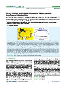
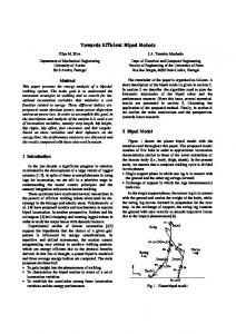
IV. Z IP W EAVE N ON -U NIFORM S AMPLING : R ATIONALE AND P OTENTIAL E FFICIENCY G AINS Due to terrain differences, we observe that not every part of a region needs the same sampling density. For example, as shown in Fig. 1a, in open places such as fields or parks the propagation path loss values do not vary much. Thus, a small number of measurement samples are sufficient to accurately interpolate and predict the coverage at unobserved locations. However, this is not the case with crowded areas where buildings may hinder unobstructed propagation of radio signals. The deflection, reflection and absorption of signals may lead to great variations in signal quality at even very small distances, for example, in city center areas (see Fig. 1b). The key idea behind ZipWeave non-uniform sampling approach is to exploit the similarity/differences in radio propagation characteristics in different sub-areas of a region in order to build reliable coverage maps with reduced number of measurements. To achieve this, we first characterize the whole region of interest by identifying geographical patches / road segments that are similar in signal strength values. This results in large sub-regions/segments at places with small variation in signal strength and small sub-regions/segments where nearby locations suffer from abrupt changes in signal quality. We then vary the sampling density across these sub-regions/segments. Such an approach provides similar coverage map prediction accuracy to its uniform (systematic-random) sampling counterpart, but with a much smaller sampling size. In this section, we demonstrate the potential savings with the ZipWeave nonuniform sampling approach (over the commonly used uniform sampling) via measurement based statistical analysis considering different cases: coverage map generation over a wide geographic area with controlled/crowdsourced measurements; and coverage along drive paths. We leave the discussion on how to realize ZipWeave non-uniform sampling in practice to the next section. A. Coverage Map for a Geographical Area First, we explore the benefit of ZipWeave non-uniform sampling approach for the case of coverage map for a wide geographical area. 1) Controlled Measurements: a) Full Enumeration Dataset: To assess the efficiency of the ZipWeave approach in this case, we will need for analysis what we refer to as a full enumeration dataset, which represents a very dense collection of measurements across the area of interest. However, it is (close to) impossible to obtain a full set of coverage measurements at all spatial locations within the geographical domain of interest. In order to generate/mimic such a dataset, we use the controlled bus dataset from Edinburgh and we identify a sub-area where we previously collected a very dense controlled set of measurements along the roads public transport buses traverse (Fig. 2a). We use these observations to interpolate/predict the signal strength values at 20,000 unobserved grid locations within this same area. We define these grid locations by segmenting the Edinburgh sub-area in 35mx35m grid cells.

4

(a) An open space area in Edinburgh.

(b) An area with tall buildings in Edinburgh.

Fig. 1: Signal strength variations in different areas. In open space (1a), the signal strength variation is small, ranging between [-9,-13] dBm. In areas with tall buildings (1b), the signal strength variation is much higher, ranging between [-4, -13] dBm.

(a) Input Dataset: Controlled Edinburgh Bus Dataset on route.

(b) Full Enumeration Dataset: Heatmap of Kriging predictions.

Fig. 2: Full Enumeration Dataset (b) generated by predicting the signal strength at 20,000 unobserved grid locations using Kriging and the Input Dataset in (a). We use the full enumeration dataset to assess the benefit with ZipWeave non-uniform sampling approach for the case of coverage map generation over a wide geographical area. The collection of 20,000 signal strength values at these grid locations represents the full enumeration dataset (Fig. 2b). We confine our subsequent analysis to this geographical subdomain for which we generated the full enumeration of signal strength readings. This, however, does not affect the nature of the results since this geographical restriction arises from the limitation in the geographic span of the controlled dataset measurement locations. b) Irregular Spatial Tessellation: We identify the geographical areas with similar signal strength observations in our analysis as follows. Data Clustering with Spatial Continuity. For non-uniform tessellation, the first step is to apply an unsupervised hierarchical clustering algorithm (i.e., HCLUST) on the signal strength values within the full enumeration dataset described above. The results show that two geographically separate clumps can be members of the same cluster since we do not run clustering on the basis of GPS locations. In order to guarantee spatial continuity within the same cluster, we then split the portions of the same cluster grouped at different geographical locations into distinct stand-alone clusters using the Connected Component Labeling (CCL) algorithm. This technique is specific to image processing by scanning an image pixel-by-pixel in order to identify regions of adjacent pixels that have similar color values. Applying CCL to the hierarchical clustering output resulted in 165 different clusters. Spatial Tessellation. Many of the 165 clusters CCL produced are, however, very small and often contained only a single observation. This happens because the signal strength at those locations is very different from its surrounding locations.

Fig. 3: Final Irregular Spatial Tessellation (reflecting the basis of ZipWeave non-uniform sampling) in an area (after applying HCLUST + CCL + KNN, we obtain 24 clusters). Such small clusters do not provide enough choice for further applying the spatial sampling plan. In order to handle this problem, we use the K-Nearest Neighbor (KNN) algorithm for appending tiny clusters with less than 30 members to the nearest large cluster. This not only reduces the number of clusters, but also confines the abrupt variations in signal strength inside a cluster (and, subsequently, corresponding geographical area). Figure 3 shows the final irregular tessellation of the area of analysis after applying KNN for merging tiny clusters into big clusters (resulting into 24 clusters). c) Results: To evaluate the benefit of the ZipWeave non-uniform sampling approach, we compare the coverage prediction accuracy with samples from the irregular clusterbased tessellation (ZipWeave ) with the one we obtain when using samples from the uniform tiling of the same geographic domain. For this, we use a calibration-validation approach

5

TABLE I: Signal strength prediction error (MAPE) using the systematic-random sampling plan (in the left) and using ZipWeave non-uniform sampling (in the right) on the controlled bus dataset from Edinburgh. Systematic-random Sampling Sample Size MAPE 360 1.00 560 0.98 640 0.85 900 0.77

ZipWeave Sample Size MAPE 480 0.74 480 0.77 480 0.76 480 0.76

TABLE II: Signal strength prediction error (MAPE) using the systematic-random sampling plan (in the left) and using ZipWeave non-uniform sampling (in the right) on the crowd dataset from Oslo. Systematic-random Sampling Sample Size MAPE 500 (25 tiles) 0.31 600 (30 tiles) 0.32 720 (36 tiles) 0.31 840 (42 tiles) 0.31

500 500 500 500

ZipWeave Sample Size MAPE (25 clusters) 0.26 (25 clusters) 0.27 (25 clusters) 0.27 (25 clusters) 0.26

and use the full enumeration dataset as ground truth. First, we separate 25% of the 20,000 regularly spaced locations in the full enumeration dataset as validation points. From the remaining 15,000 points, we select for training 20 samples from each non-uniform sub-area (for ZipWeave ) and 20 samples from each uniform tile, respectively (Fig. 4). In both cases, we use the chosen samples from each cluster or tile to be able to make a prediction at the validation points that fall inside its bounded region. We repeat this exercise four times. In the case of systematic sampling, we gradually reduce the size of tiles and record the Kriging result. In the case of the irregular spatial tessellation (ZipWeave ), we select 20 different samples per sub-area at each repetition. In Table I, we show the results of ZipWeave non-uniform sampling plan relative to the case when we use systematic sampling. Overall, we observe that ZipWeave approach achieves similar prediction accuracy to the systematic-random sampling based approach, with only half of the sample size (last row in Table I). 2) Crowdsourced Measurements: We now consider the case of generating the coverage map of a geographical area with crowdsourced measurements. For analysis in this case, to realize ZipWeave non-uniform sampling approach, we follow the same steps for irregular spatial tesselation as described in the above subsection but using the crowdsourced measurement dataset (for Oslo). We repeat the experiment as before for different sampling sizes and find that also in this case ZipWeave non-uniform sampling outperforms the commonly used systematic-random sampling approach (Table II). B. Coverage Map for a Route We now analyze the effectiveness of the ZipWeave nonuniform sampling approach for the case of predicting the coverage along a drive route, using the controlled bus dataset from Edinburgh. a) Irregular Spatial Tessellation: Though the same steps as described earlier in Sect. IV-A1 broadly apply in this case, given the intrinsic differences in the nature of the

coverage map to be generated, we apply a different set of techniques which are more effective for measurement data that follows spatial linear pattern. This is because, for instance, the connected component labeling technique is limited in its applicability to grid-based structures and it is not applicable for extracting the geographical boundaries of road segments with similar signal quality. Also, in this case, input dataset itself serves as the full enumeration dataset due to the high granularity of signal strength readings along the analyzed route. Sample Clustering and Spatial Continuity. We first apply constrained clustering for identifying the route segments with similarities in the signal strength readings. Constrained clustering is a semi-supervised clustering algorithm that takes advantage of the pair-wise relations among data points for grouping them into separate clusters. Pair-wise relations are of two types, namely must-link (indicating that two samples should be assigned to same cluster) and cannot-link (indicating the opposite). Exploiting the spatial auto-correlation of the signal strength variable, constrained clustering can group the coverage measurements such that members of same cluster are both similar in signal strength quality and are geographically adjacent, thus achieving the spatial continuity goal. For measurements over drive routes, this grouping results in tiny clusters where there are abrupt changes in the signal quality at nearby locations and larger clusters (road segments) where signal reception is similar. Constrained clustering can be parameterized with signal strength similarity threshold – a lower threshold results in more homogeneous intra-cluster members but with a high number of small-sized clusters and vice versa. For the dataset used in the analysis, we empirically determine the right threshold setting to be equal to difference of up to 6 Arbitrary Signal Unit (ASU), which generated 365 clusters with most of them having very few members. Spatial Tessellation. As with the earlier cases, we merge the geographically close tiny clusters (i.e. clusters with few members) irrespective of their signal quality using Density Based Spatial Clustering of Applications with Noise (DBSCAN). DBSCAN extracts arbitrary-shaped clusters from points in space that are closely packed together. It requires specification of the minimum number of neighbors that a data point should have within a particular radius so that to term this neighborhood as a cluster; we set the radius of the neighborhood to be 50 meters and the minimum number of neighbors to be 5. The resulting re-clustering (Fig. 5) reduced the number of cluster from 365 down to 38, 13 of which are produced by DBSCAN while the rest are large clusters generated by constrained clustering. b) Results: Table III compares prediction accuracy with ZipWeave non-uniform sampling and systematic-random sampling for different sample sizes for the dataset shown in Fig. 2 (a). It must be noted that the number of samples retrieved from each cluster and tile are equal in size, namely 20 samples. For systematic-random sampling, we decrease the tile size in each repetition and we only filter the tiles having at least 20 samples. In both the clustering and tile based approaches, we

6

(a) ZipWeave non-uniform Sampling.

(b) Systematic-random Sampling.

Fig. 4: Calibration set (sample) size chosen by (a) ZipWeave non-uniform sampling and (b) Systematic-random sampling approaches for the same prediction accuracy (MAPE). We can visually confirm the difference on the sample sizes. V. Z IP W EAVE N ON -U NIFORM S AMPLING IN P RACTICE

Fig. 5: Final irregular tessellation (reflecting the basis of ZipWeave non-uniform sampling) on routes (after applying Constrained Clustering + DBSCAN, we obtain 38 route segments). TABLE III: Signal strength prediction error (MAPE) using systematic-random sampling (in the left) and ZipWeave nonuniform sampling on a route (in the right) on the controlled bus dataset from Edinburgh. Systematic-random Sampling Sample Size MAPE 660 2.64 720 2.44 980 2.26 1,100 2.24

ZipWeave Sample Size MAPE 600 2.07 600 1.84 600 1.89 600 1.85

apply Kriging with leave-one-out cross validation (LOOCV) per cluster and tile respectively. The differences in signal strength quality within a same DBSCAN based cluster makes it obvious that samples from such a cluster cannot predict well the unobserved locations of its cluster. From multiple tests we run on datasets from different buses operating in Edinburgh (not stated here), the overall prediction accuracy decreases when DBSCAN-based clusters are also considered for sampling along with the constrained-based clusters so that to predict signal quality in the rest of their cluster locations. Even with this decrease, nonuniform sampling still outperforms systematic-random sampling approach in terms of coverage prediction accuracy. This improvement (shown by results of Table III) confirms that nonuniform cluster-based sampling produces better coverage maps due to factoring in the varying sampling density requirement of the terrain under consideration.

A good spatial sampling strategy design recognizes the heterogeneity in the mobile coverage and tries to account for it by choosing the sampling locations driven by a suitable criterion/metric that helps boost the accuracy of the empirical coverage maps. Analysis in the last section confirmed the opportunity for efficient coverage map generation via nonuniform sampling exploiting the sub-regions with similar radio propagation characteristics but without regard to practical constraints (e.g., assuming access to full enumeration dataset). In this section, we consider the realistic scenario where the entity interested in generating empirical mobile coverage maps may not have a-priori information about the coverage characteristics of the region in question. Targeting this scenario, we propose a simple and practical non-uniform spatial sampling methodology to identify the locations where the measurements are most needed. Our sampling optimization is aimed at reducing the measurement cost with no adverse impact on the prediction accuracy. This is because collecting drive test measurements is known to be labor- and costintensive. Similarly, for crowdsourced measurements, not all measurement readings may raise accuracy but instead deplete battery life and impact the data quota of the MBB customer. Following common practice, we propose a two-phase sampling design. For the first phase, we use systematic-random sampling. We divide the area into equally sized tiles and randomly select the same (few) number of samples from each tile. For the second phase, a naive approach is simply to repeat another round of systematic random sampling per tile but it foregoes the opportunity to optimize the overall sample size needed for producing a reliable coverage map. So we need a more sophisticated approach that leverages the insights from the analysis in the previous section. To that end, we first discuss the criterion that appears to be most promising for deciding representative sampling locations. We then investigate a non-uniform sampling strategy based on the selected criterion. A. Metric to Guide Second Phase Sample Selection For interpolation, Kriging exploits autocorrelation—that is, the statistical relationships among the measured points. Because of this, it not only produces a prediction surface, but

7

also provides some measure of the accuracy of the predictions in the form of Kriging Variance (KV). KV is a common metric for determining where to sample more [15]. However, KV is a global measure of variance as it is based on the configuration of the data and of the variogram, and does not reflect the local variance. Hence, it is homoescedastic and may prove untrustworthy when there is a lack of stationarity accross the region of interest [17]. Interpolation Variance (IV) (also termed as Local Error Variance) [17] is an alternative to KV and has some correlation with the absolute prediction error which KV lacks. We evaluate the effectiveness of these metrics using two different datasets: the crowd dataset from Oslo and the controlled dataset from Edinburgh. For each dataset, we perform systematic-random sampling to have first phase samples. We then compare two cases corresponding respectively to the use of KV and IV metrics to select the tiles that need more sampling to increase the accuracy of the coverage map. To assess the relationship between KV/IV and prediction error, we can leverage the ground-truth measurements from the datasets at the predicted locations. Results shown in Fig. 6 indicate that neither KV nor IV exhibit good correlation with prediction error in our context of coverage prediction and mapping. To overcome the ineffectiveness of commonly used metrics (KV and IV) for guiding second phase sample selection, we propose to use as indicator for prediction accuracy the Kriging absolute prediction error itself. This metric, however, needs prior knowledge about the actual signal strength values at the predicted locations to calculate the prediction error. We therefore employ the LOOCV approach for Kriging performance evaluation using first phase samples. The prediction errors we obtain form the basis for driving subsequent phase of sampling, as we describe in more detail below.

TABLE IV: Signal strength prediction error when considering systematic-random sampling (in the left) and ZipWeave ’s non-uniform sampling using a MAPE-proportional probability raster (in the right). Systematic-Random Sampling Sample Size MAPE 880 1.19 1,580 1.15 2,257 1.10 2,917 1.09 3,574 1.08

ZipWeave Non-Uniform Sampling Sample Size 880 1,193 1,427 1,737 1,967

MAPE 1.19 1.13 1.09 1.07 1.04

coverage map. In non-uniform sampling, we map a probability raster to sub-regions of the overall region of interest; we assume sub-regions to be same sized tiles for ease of practical realization. The values in the probability raster correspond to the Mean Absolute Prediction Error (MAPE) resulted from applying Kriging with LOOCV per tile. Further we set to zero the probability raster values of the tiles with MAPE lower than average MAPE of all the tiles. MAPEs of the remaining tiles are normalized such that probability raster sums up to 1. The number of samples drawn from each tile in the next phase is proportional to their value in the probability raster. This approach results in non-uniform samples per tile unlike the systematic sampling where equal number of samples are retrieved from each tile per sample phase. The non-uniform sampling approach thus leads to reduced costs and/or increased coverage map accuracy by targeting the areas with higher need for subsequent sampling. C. Evaluation

Creating an optimal sampling design requires finding the right balance between the accuracy of prediction (requiring more samples) and the cost of sampling (limiting the number of samples and corresponding costs of gathering them). As already demonstrated in the previous section, given the terrain and urban landscape differences, not every part of the region of interest needs similar sampling density2 . Thus, to accommodate the spatial heterogeneity of cellular coverage, we propose to employ for second phase sampling a non-uniform sampling approach that exploits the notion of probability raster used by Balanced Sampling [18]. The probability raster is a vector with size equal to the number of sub-areas within the region of interest such that each value indicates the importance of a sub-area with respect to the sampling objective. The essential idea behind non-uniform sampling is to identify sub-regions that have a high level of uncertainty for coverage prediction and increase the density of sampling in those sub-regions to implicitly increase the accuracy of the

We now evaluate ZipWeave non-uniform sampling strategy by applying Ordinary Kriging on the sampled crowd dataset from Oslo3 . To quantify accuracy of the resulting coverage map in each case, we evaluate the Mean Absolute Prediction Error (MAPE) for the Ordinary Kriging based spatial interpolation of coverage. We compare the use of non-uniform sampling in the second phase with that of using systematicrandom sampling by contrasting the coverage interpolation results. Recall that we use systematic-random sampling for first phase sampling in both plans. We consider 50 Km x 50 Km square area spanning Oslo and divide it into 1 Km x 1 Km sized tiles forming individual sub-regions. From the Oslo crowd dataset, we randomly pick 20 samples per tile to start with as part of systematic-random sampling in the first phase. For the baseline approach, we use the same kind of systematic-random sampling for the second phase, i.e., we attempt to randomly select 20 additional samples per tile in the second phase (all available samples in a tile are used when there are fewer than 20 unused remaining samples in the dataset). For ZipWeave (non-uniform sampling), we build the probability raster in the second phase based on Kriging prediction errors computed using LOOCV with samples from the first phase. The sample size per tile in second

2 Note however that sparse systematic random sampling is helpful when starting to sample (first phase) to get a sense of the region of interest in terms of ability to accurately predict coverage.

3 Although we present results with the crowd dataset from Oslo to showcase the benefits of non-uniform sampling, similar results apply for the other controlled and crowd datasets.

B. ZipWeave Non-Uniform Sampling Strategy

8

(a) Oslo Crowd Dataset.

(b) Edinburgh Controlled Dataset.

Fig. 6: Poor correlation of KV and IV with Absolute Prediction Error of predicted signal strength. phase is proportional to per tile value in the probability raster (or equivalently MAPE). In Table IV, we present the average prediction errors, across the whole region, while using both the non-uniform and systematic-random sampling schemes. We observe that the accuracy of the coverage prediction is similar or better in all phases with non-uniform sampling scheme. Even more, the results show that by using non-uniform sampling, we can achieve equivalent prediction accuracy compared to the baseline approach with only about half the sample size. These results match those from the analysis in the previous section, demonstrating that the practical form of ZipWeave non-uniform sampling described in this section is able to achieve expected gains in sampling efficiency. VI. Z IP W EAVE : F USING DATA FROM D IFFERENT S OURCES Availability of both crowdsourced and controlled measurements at certain regions brings forth the question of their combined usage for coverage prediction. The wider geographical span of crowdsourced measurements and greater reliability of controlled measurements suggests that utilizing both datasets can raise accuracy of coverage prediction in a region. With this in mind, the focus of the weaving part of ZipWeave is on the fusion of different type of datasources from same region. To this end, we use both the crowd and the controlled datasets we collect in Oslo and compare the coverage prediction accuracy in the same spatial domain when using as input the two datasets separately and then their union. For both datasets, the network technology mode is the same (i.e., 4G/LTE) and the unit of signal strength matches (RSRQ in dBm). In order to evaluate the accuracy of prediction with regard to both the datasets, we select the crowdsourced measurements only from the area near the measurement routes in the controlled train dataset. We further focus our analysis on the geographical domain where both measurement approaches have significant amount of samples. We divide the route into tiles and only consider the tiles where both the crowd and controlled data are present. This sums up 22 such tiles. Further, to ensure equal representation of each tile, we retrieve equal proportion of calibration and validation samples from each of the tiles. We consider 3 different calibration set configurations, namely crowd training data only (approximately 1,000

TABLE V: Absolute prediction errors after using Ordinary Kriging on three different configurations of the calibration/validation dataset. Test No. 1 2 3

Crowdsourced 2.59 2.45 2.53

Controlled 2.45 2.83 2.57

Datasets Union 2.28 2.25 2.25

samples), controlled training data only (approximately 1,000 samples) and containing equal representation from crowd and controlled datasets (i.e., approximately 500 form each). The validation also contains samples from both the datasets with equal representation (i.e., 500 from each). We then apply Kriging on validation samples by using crowdsourced calibration samples, controlled calibration samples and the calibration set which has representation of both. We perform three repetitions of the test by reselecting the samples in all the above cases and performing interpolation. The results we present in Table V reveal that, in all the three tests, the combination of both the datasets outperforms the cases when we use a single data source. The improvement is, however, marginal because the range of signal strength values from the datasets is both narrow and similar (i.e with first quartile -6dBm and third quartile 9dBm). Also, we confine our analysis to a limited geographical domain in Oslo because of the limitations of the controlled dataset in that location4 . Once the efficiency of using combination of the datasets is obvious, we evaluate the non-uniform sampling strategy against the systematic-random one for boosting the coverage map accuracy. To this end, we first combine both the crowdsourced and controlled datasets into one union dataset. Then, we retrieve at most 30 samples from each of the 22 tiles by choosing 547 samples in total for the first phase of samples. After applying interpolation with cross-validation on each tile separately we move to the second phase of samples. For systematic-random sampling we again retrieve equal number of samples (i.e. at most 30) from each of the tiles, thus making the total sample size equal to 968 datapoints. For the ZipWeave non-uniform sampling plan, as described in the previous section, we exploit the first-phase mean absolute prediction error metric of each tile and generate probability 4 We could not this exercise using the datasets from Edinburgh due to incompatibility in the signal strength parameters in the two datasets.

9

TABLE VI: Absolute prediction errors, after using Ordinary Kriging four different times with systematic-random and nonuniform sampling plans. Test No.

1 2 3 4

SystematicRandom Sampling Phase 1 2.02 (547) 1.98 (547) 2.06 (547) 2.09 (547)

SystematicRandom Sampling Phase 2 1.99 (968) 1.92 (968) 2.02 (968) 2.05 (968)

Non-Uniform Sampling Phase 2 1.94 1.89 1.98 1.98

(650) (631) (669) (677)

raster on this information to point out the tiles where more drilling might decrease the overall prediction errors. We repeat this test four times with different initial and additional sample sets. Table VI summarizes the results of the four different coverage tests. In all the four tests, we observe that nonuniform sampling results in better accuracy with fewer samples than its systematic sampling counterpart, demonstrating the effectiveness of ZipWeave in its full form. VII. C ONCLUSIONS In this paper, we have proposed ZipWeave, a framework for efficient and reliable mobile coverage map generation. ZipWeave employs non-uniform sampling to reduce the number of measurements while not compromising coverage prediction accuracy, essentially by exploiting the similarity in radio propagation characteristics within sub-regions of the area of interest. It also aims to take advantage of the synergy of different types of measurement data that may be available in a given region by fusing them in coverage map generation process. Our extensive measurement based statistical analysis has shown that non-uniform sampling on the basis of clusters and segments having similar signal quality produces better prediction accuracy with almost half the samples required by the commonly used systematic-random sampling scheme. We also obtain similar gains with a practical form of ZipWeave non-uniform sampling strategy that does not assume any prior information of the region of interest. The other aspect of ZipWeave to complement the reliability of controlled, drivetest like, measurements with the crowdsourced measurements with a wider geographical spread is shown to result in a more reliable coverage map. One key aspect for future work is to accommodate the time dimension in the ZipWeave framework, i.e., to examine the evolution of the measurement-based coverage map over time during the course of day/week and across longer periods accounting for infrastructure/environment changes. Another avenue for future work is to examine the potential for generating more accurate coverage maps from knowledge of infrastructure locations (cell towers). ACKNOWLEDGMENTS We thank OpenSignal and Philip Lock at Edinburgh Lothian Buses for providing access to the datasets used in this work. This work was partially supported by the European Union’s Horizon 2020 research and innovation program under grant agreement No. 644399 (MONROE) and by the Norwegian

Research Council under grants 250679 (MEMBRANE). The views expressed are solely those of the authors. We would like to thank NSB for hosting measurement nodes aboard their operational passenger trains. R EFERENCES [1] C. Phillips, D. Sicker, and D. Grunwald, “A survey of wireless path loss prediction and coverage mapping methods,” IEEE Communications Surveys & Tutorials, vol. 15, no. 1, 2013. [2] “Open Signal Inc.” http://opensignal.com/. [3] J. Johansson, W. A. Hapsari, S. Kelley, and G. Bodog, “Minimization of drive tests in 3GPP release 11,” IEEE Communications, vol. 50, no. 11, 2012. [4] “MobiPerf,” http://www.mobiperf.com/. [5] M. K. Marina, V. Radu, and K. Balampekos, “Impact of indooroutdoor context on crowdsourcing based mobile coverage analysis,” in Proc. ACM SIGCOMM 2015 Workshop on All Things Cellular: Operations, Applications and Challenges, 2015. [6] S. Kolyaie, M. Yaghooti, and G. Majidi, “Analysis and simulation of wireless signal propagation applying geostatistical interpolation techniques,” Archives of Photogrammetry, Cartography and Remote Sensing, vol. 22, no. 1, 2011. [7] C. Philips et al., “Practical radio environment mapping with geostatistics,” in 2012 IEEE International Symposium on Dynamic Spectrum Access Networks, 2012. [8] M. Molinari, M. Fida, M. K. Marina, and A. Pescape, “Spatial interpolation based cellular coverage prediction with crowdsourced measurements,” in Proc. ACM SIGCOMM 2015 Workshop on Crowdsourcing and crowdsharing of Big (Internet) Data, 2015. [9] T. Hengl, “A practical guide to geo-statistical mapping,” Second, extended edition of the EUR 22904 EN Scientific and Technical Research series report, 2009. [10] B. e. a. Sayrac, “Bayesian spatial interpolation as an emerging cognitive radio application for coverage analysis in cellular networks: Bayesian Spatial Interpolation for Coverage Analysis,” Transactions on Emerging Telecommunications Technologies, vol. 24, no. 7-8, Nov. 2013. [11] W. R. Tobler, “A computer movie simulating urban growth in the detroit region,” Economic geography (Supplement: Proceedings. International Geographical Union. Commission on Quantitative Methods), vol. 46, 1970. [12] S. Grimoud, B. Sayrac, S. B. Jemaa, and E. Moulines, “Best sensor selection for an iterative rem construction,” in 2011 IEEE Vehicular Technology Conference, Fall, 2011. [13] R. Olea, “Sampling design optimization for spatial functions,” Journal of the international Association for Mathematical Geology 16.4, vol. 16, no. 4, 1984. [14] E. Delmelle and P. Goovaerts, “Second-phase sampling designs for non-stationary spatial variables,” Geoderma, vol. 153, no. 1-2, 2009. [15] D. J. Brus and G. Heuvelink, “Optimization of sample patterns for universal kriging of environmental variables,” ScienceDirect, Geoderma, vol. 138, no. 1–2, 2007. [16] A. Kvalbein, D. Baltr¯unas, J. Xiang, K. R. Evensen, A. Elmokashfi, and S. Ferlin-Oliveira, “The Nornet Edge platform for mobile broadband measurements,” Elsevier Computer Networks special issue on Future Internet Testbeds, 2014. [17] J. K. Yamamoto, “An alternative measure of the reliability of ordinary kriging estimates,” Mathematical Geology, vol. 32, no. 4, 2000. [18] K. Krivoruchko and K. Butler, “Unequal-probability based spatial sampling,” http://www.esri.com/esri-news/arcuser/, 2013.