Drag Reduction of a Turbulent Boundary Layer over an Oscillating ...

Hindawi Publishing Corporation International Journal of Aerospace Engineering Volume 2015, Article ID 891037, 9 pages http://dx.doi.org/10.1155/2015/891037

Research Article Drag Reduction of a Turbulent Boundary Layer over an Oscillating Wall and Its Variation with Reynolds Number Martin Skote, Maneesh Mishra, and Yanhua Wu School of Mechanical & Aerospace Engineering, Nanyang Technological University, 50 Nanyang Avenue, Singapore 639798 Correspondence should be addressed to Martin Skote; [email protected] Received 31 August 2015; Revised 18 November 2015; Accepted 24 November 2015 Academic Editor: Paul Williams Copyright © 2015 Martin Skote et al. This is an open access article distributed under the Creative Commons Attribution License, which permits unrestricted use, distribution, and reproduction in any medium, provided the original work is properly cited. Spanwise oscillation applied on the wall under a spatially developing turbulent boundary layer flow is investigated using direct numerical simulation. The temporal wall forcing produces a considerable drag reduction over the region where oscillation occurs. Downstream development of drag reduction is investigated from Reynolds number dependency perspective. An alternative to the previously suggested power-law relation between Reynolds number and peak drag reduction values, which is valid for channel flow as well, is proposed. Considerable deviation in the variation of drag reduction with Reynolds number between different previous investigations of channel flow is found. The shift in velocity profile, which has been used in the past for explaining the diminishing drag reduction at higher Reynolds number for riblets, is investigated. A new predictive formula is derived, replacing the ones found in the literature. Furthermore, unlike for the case of riblets, the shift is varying downstream in the case of wall oscillations, which is a manifestation of the fact that the boundary layer has not reached a new equilibrium over the limited downstream distance in the simulations. Taking this into account, the predictive model agrees well with DNS data. On the other hand, the growth of the boundary layer does not influence the drag reduction prediction.

1. Introduction Turbulence in an ubiquitous phenomena in aerospace applications is, more often than not, detrimental for the performance of, for example, aircrafts. In particular, the skin friction, which produces about half of the total drag, continues to be a challenge to decrease by means of flow control. Strategies for achieving drag reduction are broadly classified as either active or passive. Active mechanisms are further classified as closed loop or open loop type, depending on whether feedback from the flow is used for calculating the control actuation. Considerable progress both in the understanding of drag reduction mechanisms and in the development in techniques for obtaining drag reduction has been made in the past ten years. This progress has been made possible by the advancement of computer capabilities and more or less imaginative control strategies. Spanwise wall oscillations are an active mechanism for achieving high drag reductions which has the attractive property of being open loop and thus lends itself suitable for practical implementation without the need for complicated sensors to detect the flow state.

However, two outstanding issues remain before any active control mechanism can be implemented in real engineering applications. Firstly, the power to drive the control is still much higher than the power gained from drag reduction. This may be addressed by novel techniques replacing the actual motion of the wall, for example, plasma actuators [1, 2], Lorentz force [3, 4], or dielectric electroactive polymers [5]. Secondly, when moving from low Reynolds number in the computer or laboratory setting to the high Reynolds number in real applications, the effect on the drag reduction efficiency is not known. This second issue is in the context of aerospace applications equally important as the first one and is the topic of the present investigation. Ever since the first studies of turbulent flow in a channel with wall oscillations using direct numerical simulation (DNS) by Jung et al. [6], the topic has been slowly progressing towards higher Reynolds numbers [7–9]. The latest work on this topic has been completely focused on channel flow, including the more analytical work by [10]. For a list of references to work done between the pioneering study and

2

International Journal of Aerospace Engineering

the later ones mentioned above, please refer to, for example, [11] which utilizes data from many different investigations. The influence of Reynolds number on DR is an important question for practical implementation aspects. This is still an open question and a clear understanding of the Reynolds number dependence of DR is presently lacking. Results from previous channel flow investigations with near-optimal oscillation parameters suggest a relation of the form DR ∼ Re𝛼𝜏 ,

(1)

where Re𝜏 = ℎ𝑢𝜏 /] is the Reynolds number based on channel half width (ℎ), friction velocity (𝑢𝜏 ), and kinematic viscosity (]). This relation was first suggested by Choi et al. [12]. Channel flow simulations with optimal oscillation parameters have subsequently suggested that 𝛼 = −0.2. However, as indicated by Gatti and Quadrio [13], the value of the exponent in relation (1) is most probably dependent on the oscillation parameters; thus a universal relation will be unattainable. In addition, in the study of the Reynolds number averaged Navier-Stokes equations using a perturbation analysis by Belan and Quadrio [14], it is found that a relation of the type DR ∼ 𝛾 + Re𝛼𝜏

(2)

matches the data better. Hence, the DR approaches a constant value as Re𝜏 → ∞. Most of the previous DNS studies have focused on channel flow with the benefits of periodic boundary conditions which reduce the computational costs. However, not much work has been done to explore the effects on a turbulent boundary layer using numerical simulations. Note that the local drag reduction decreases downstream for a spatially growing boundary layer flow in contrast to the channel flow where drag reduction remains constant in both time and space after attaining an equilibrium value. The same numerical code used for the present investigation has previously been used for both temporal and spatial oscillations of the wall under a turbulent boundary layer [15–17]. Recently, Lardeau and Leschziner [18] reported their findings for boundary layer flows using DNS where they focused on the transition of the skin friction to a steady low-drag state and perform phase-averaged analysis of turbulent statistics. In passing we also note that the wall oscillation technique has been utilized for transition control in the boundary layer; see [19–21]. Regarding practical applications, the oscillating wall technique may be still far from being matured. With the existing technological capabilities available, it is hard to imagine large portions of the aircraft wing or fuselage surface oscillating. However, since other methodologies, based on passive control such as riblets, have yet to be commonplace, the prospect of other methods based on active control, possibly refined by feedback control in order to increase their energy saving capacity, should be considered for future applications. In passing, one may furthermore note that the field of active flow control is open to new innovative ideas, although based on oscillating wall motion. One example is the rotating disc idea pursued by Ricco and his group [22, 23].

Although laminar flow is prevalent in many applications, for example, biochemistry [24] or biology [25], which allows for numerical simulations using the Navier-Stokes equations, turbulent flow is always encountered in aerospace applications. If realistic Reynolds numbers are considered when performing numerical work, the Navier-Stokes equations will not be possible to solve due to the wide range of scales (as measured by the Reynolds number) present in the flow. Hence, turbulence modelling will be required and either the Reynolds Average Navier-Stokes equations (RANS) or Large Eddy Simulations (LES) need to be employed. However, for the phenomena of drag reduction due to wall forcing, as investigated in this work, there is no reliable turbulence model available. Hence, we focus on low Reynolds number flow which, although turbulent, can be numerically simulated using DNS, that is, by obtaining the solution to the NavierStokes equations without any turbulence modelling. Only after understanding how the turbulence is affected by the wall forcing, a model which can be used for higher Reynolds number engineering application may be developed. For the purpose of DNS, highly efficient and accurate numerical schemes based on spectral methods have been employed in this work. The rest of the paper is organized as follows. In Section 2, the numerical scheme and simulation parameters are presented. The results are discussed in Section 3, which first concerns older data found in the literature in Section 3.1. Based on previous simulations and experiments, a predictive relation for DR at high Reynolds numbers is suggested, which differs from the general conclusion of a Reynolds number dependency according to (1). Then, in Section 3.2, a predictive formula based on the shift of the velocity profile in drag-reduced flows is derived and compared with the new simulation results. In Section 3.3 the velocity profile shift is further investigated and the implications of the results are related back to the findings in Section 3.2. Lastly, conclusions are mentioned in Section 4.

2. Numerical Method and Simulation Parameters The numerical code used, SIMSON (A Pseudo-Spectral Solver for Incompressible Boundary Layer Flows), was originally developed at KTH, Stockholm [31]. An outline of the numerical scheme is presented in Section 2.1; the various parameters used and the resolution are presented next in Section 2.2, where also the implementation of the wall motion is discussed. 2.1. Numerical Scheme. A pseudospectral method with Fourier discretization in the streamwise and spanwise directions and Chebyshev polynomials in the wall-normal direction has been used. The simulations are started with a laminar boundary layer at the inflow. A random volume force near the wall at the beginning of the computational domain is used to trigger the flow to transition. At the end of the domain, a fringe region is added to enable simulations of spatially developing flows. The flow in this region is forced from the outflow of the physical domain to the inflow. In this way the physical domain and the fringe


3 Table 1: Numerical parameters for the simulations presented. 𝐿 and 𝑁 refer to the size (measured in displacement thickness at 𝑥 = 0) and the number of modes, respectively.

1

𝐿𝑥 2400

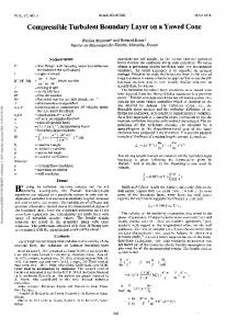
f(x)

0.8 0.6

𝐿𝑦 75

𝐿𝑧 34

𝑁𝑦 301

𝑁𝑧 144

Δ𝑥+ 15.8

+ Δ𝑦min 0.04

Δ𝑧+ 4.96

y, v wall-normal

0.4

x, u streamwise

0.2 0

𝑁𝑥 3200

W = Wm sin(𝜔t) 0

2

4

6

8

10

z, w spanwise

x Fringe region

Figure 1: Function 𝑓(𝑥) with Δ𝑥rise = Δ𝑥fall = 3.

Zone of oscillation

region together satisfy periodic boundary conditions. The implementation is done by adding a volume force, 𝑢𝑖 − 𝑢𝑖 ) , 𝐹𝑖 = 𝜆 (𝑥) (̃

(3)

to the Navier-Stokes equations: 2

𝜕𝑢 𝜕𝑢 𝜕𝑢𝑖 1 𝜕𝑝 + ] 2𝑖 + 𝐹𝑖 . + 𝑢𝑗 𝑖 = − 𝜕𝑡 𝜕𝑥𝑗 𝜌 𝜕𝑥𝑖 𝜕𝑥𝑗

(4)

The force 𝐹𝑖 applies to the fringe region only where 𝜆(𝑥) is the strength of the forcing and 𝑢̃𝑖 is the laminar inflow velocity profile to which the solution 𝑢𝑖 is forced. The fringe function is required to have minimum upstream influence and is designed as 𝜆 (𝑥) = 𝜆 max 𝑓 (𝑥) ,

(5)

𝑥 − 𝑥end 𝑥 − 𝑥start ) − 𝑆( + 1) . Δ𝑥rise Δ𝑥fall

(6)

with 𝑓 (𝑥) = 𝑆 (

Here 𝜆 max is the maximum strength of the fringe, 𝑥start and 𝑥end denote the spatial extent of the region where the fringe is nonzero, and Δ𝑥rise and Δ𝑥fall are the rise and fall distance of the fringe function, respectively. Figure 1 shows how the fringe function varies with 𝑥 with Δ𝑥rise = 3 and Δ𝑥fall = 3. 𝑆(𝜂) is a continuous step function that varies from zero for 𝜂 ≤ 0 to unity for 𝜂 ≥ 1 and is given by 0, 𝜂 ≤ 0, { { { { 1 𝑆 (𝜂) = { , 0 < 𝜂 < 1, (1/(𝜂−1)+1/𝜂) { ) { (1 + 𝑒 { 𝜂 ≥ 1. {1,

(7)

The advantage of this expression is that 𝑆(𝜂) has continuous derivatives of all orders. The function 𝑓(𝑥) is also used in enforcing the wall oscillation boundary condition as described in Section 2.2.

U∞ Trip

Transition region

Figure 2: Illustration for the problem setup.

The time integration is performed using a third-order Runge-Kutta scheme for the nonlinear terms and a secondorder Crank-Nicolson method for the linear terms. A 3/2-rule is applied to remove aliasing errors from the evaluation of the nonlinear terms when calculating FFTs in the wall parallel plane. 2.2. Numerical Parameters. All quantities are nondimensionalized by the free stream velocity (𝑈∞ ) and the displacement thickness (𝛿∗ ) at the starting position of the simulation (𝑥 = 0), where the flow is laminar. The Reynolds number is set by specifying Re𝛿∗ = 𝑈∞ 𝛿∗ /] at the laminar inlet (𝑥 = 0). Wall oscillation is imposed over a long segment of the wall to examine the influence of ReΘ (ReΘ = 𝑈Θ/], Θ being the momentum thickness) on DR. Table 1 gives the different parameters chosen for the computational box and grid. The length of the computational box is given in simulation length ∗ ). The resolution used for the simulations is shown units (𝛿𝑥=0 in + units. Note that unless otherwise stated the + superscript indicates that the quantity is made to be nondimensional with the friction velocity of the unmanipulated boundary layer (the reference case), denoted as 𝑢𝜏0 , and the kinematic viscosity (]). Note that 𝑢𝜏0 is varying with 𝑥. In the calculation of the resolution, a representative 𝑢𝜏0 is taken from a position 𝑥 = 2/3𝐿 𝑥 , where 𝐿 𝑥 is the length of the computational box, which corresponds to the location where the oscillating region ends. The grid resolution is consistent with other DNS, which has been proven to be sufficient [29]. In addition, with the same resolution and Reynolds number another case was simulated for which experimental data exist [28] and almost perfect agreement was obtained with respect to both magnitude and spatial development; see [26]. An illustration for the current problem setup is shown in Figure 2. After an initial trip of the flow, the flow undergoes

4


transition to fully turbulent flow. The tripping has been described in detail in [29] and the quality of this methodology ¨ u [30]. has been thoroughly investigated by Schlatter and Orl¨ A section of the resulting turbulent flow is then subjected to wall oscillations, as described below. At the end of the domain, there is a fringe region to satisfy periodic boundary condition as discussed in the previous section. Minimal upstream influence is ensured by the design of the fringe function [31]. The implementation of the oscillating spanwise wall velocity is identical to the one used in [29]. The wall oscillation is applied in the spanwise direction at a particular region in streamwise direction. Therefore, a profile function 𝑓(𝑥) is utilized to define the domain where the oscillation occurs. Furthermore, the gradual increase of the profile function prevents the spurious oscillations (Gibb’s phenomena) which might otherwise be introduced due to a discontinuous jump in the velocity around the starting point of wall forcing. The form of the wall velocity boundary condition is given by 𝑊|𝑦=0 = 𝑓 (𝑥) 𝑊𝑚 sin (𝜔 (𝑡 − 𝑡start )) ,

(8)

where 𝑓(𝑥) is the same profile function as that used for fringe region; see (6); and 𝑊𝑚 is the maximum wall velocity. The parameter 𝜔 is the angular frequency of the wall oscillation, which is related to the period through 𝜔 = 2𝜋/𝑇. The parameter 𝑡start determines when the oscillation starts. The sampling time for the reference case was 24800 in ∗ /𝑈∞ ) and started only after a stationary flow time units (𝛿𝑥=0 (in the statistical sense) was reached after 13200 time units. In the cases with wall forcing, the reference case was used as the initialized flow field and additional 4300 time units were simulated before statistics were sampled during another 33000 time units, corresponding to 478 periods of oscillation. The parameter 𝑡start in (6) is 38000 (= 13200 + 24800). In the simulations presented here, the angular frequency (𝜔) of the wall oscillation is set to 0.09099 and maximum wall velocity (𝑊𝑚 ) is set as 0.5028, which in wall units corresponds to 𝑇+ = 76.4 and 𝑊𝑚+ = 10.7, calculated as 𝑊𝑚+ = 𝑊𝑚 /𝑢𝜏0 and 𝑇+ = 𝑇(𝑢𝜏0 )2 /], based on 𝑢𝜏0 at the start of oscillations (𝑥 = 500), which is equal to 0.047. Note that the value of 𝑊𝑚+ and 𝑇+ changes with streamwise position because local 𝑢𝜏0 varies, whereas 𝑊𝑚 and 𝑇 are kept fixed. At the end of the oscillating part (𝑥 = 1600) the friction velocity of the reference case is 𝑢𝜏0 = 0.042 and gives a value of 𝑊𝑚+ = 12.0 and 𝑇+ = 60.8 at that position. The parameters pertaining to the oscillations are summarized in Table 2.

3. Results Before presenting the results in Sections 3.1 to 3.3, various definitions needed in the following are presented. The friction velocity is defined as 𝑢𝜏 ≡ √ ]

𝜕𝑢 󵄨󵄨󵄨󵄨 󵄨 , 𝜕𝑦 󵄨󵄨󵄨𝑦=0

where ] is the kinematic viscosity.

(9)

Table 2: Parameters regarding the wall oscillations for the simulation presented. 𝑊𝑚+ 10.7

𝑇+ 76.4

𝑥start 500

𝑥end 1600

ReΘstart 963

ReΘend 1989

The resulting drag reduction (DR) is calculated from DR (%) = 100

𝐶𝑓0 − 𝐶𝑓 𝐶𝑓0

,

(10)

where 𝐶𝑓0 = 2(𝑢𝜏0 /𝑢∞ )2 is the skin friction of the reference case. An alternative expression of the DR will in this paper be used according to D=

𝐶𝑓0 − 𝐶𝑓 𝐶𝑓0

.

(11)

Hence, we may write 2

𝑢 D = 1 − ( 𝜏0 ) . 𝑢𝜏

(12)

3.1. Drag Reduction in Channel and Boundary Layer Flows. In this section focus will be on the maximum DR in the boundary layer and its dependency on the Reynolds number where the oscillation starts. In addition, data from channel flow DR in the literature will be utilized as there are more data to compare with for this flow geometry. Note that one unique DR value exists for a channel flow, while the DR is varying downstream for a boundary layer. Hence, in order to compare the two cases, we specify the maximum DR in boundary layer case for comparison with channel flow data. Three different sets of channel flow data will be presented here. They are chosen because up to four different Reynolds numbers have been investigated for identical oscillation parameters. For comparison with the boundary layer it is necessary to convert the Reynolds number used in channel flow configuration, Re𝜏 , to ReΘ , which is done by using the relation , Re𝜏 = 1.13Re0.843 Θ

(13)

¨ u [32]. as given by Schlatter and Orl¨ The data is presented in Figure 3 and is colour-coded according to the oscillation parameters used in the DNS/ experiments. Note that black, red, and magenta constitute separate sets of parameters, while green, blue, and cyan are data from investigations using identical values of 𝑊𝑚+ = 12 and 𝑇+ = 100. In addition, data from DNS/experiments is indicated by symbols, while the solid and broken lines represent the relations proposed. The boundary layer data shown in Figure 3 as circles is taken from [26] and is compared with channel flow (cross) from the DNS by [27] as well as experimental boundary layer data (plus) from [28]. The DNS data from [26] show


5

50

Table 3: Parameters for the profiles presented in Figure 3.

40

Line type

DR

30

20

𝛽

𝐴/ReΘ + 𝐵 Solid

𝐶ReΘ Broken

Colour

𝑊𝑚+

𝑇+

𝐴

𝐵

𝐶

𝛽

Black Red Green Blue

11.3 10.0 12.0 12.0

67.0 50.0 100.0 100.0

2884 2679 7143 5068

23.44 20.12 21.97 27.66

140 111

−0.22 −0.17

10

0

0

1000

2000

3000 ReΘ

4000

5000

6000

𝛽

Figure 3: DR as a function of ReΘ . (–) Profiles according to (14). (– –) Profiles according to (15). Black colour indicates data for oscillations with 𝑊𝑚+ = 11.3 and 𝑇+ = 67: ( ⃝ ) DNS from [26], (×) for channel flow from [27], and (+) for boundary layer experiments from [28]. Red colour indicates data for oscillations with 𝑊𝑚+ = 10 and 𝑇+ = 50: (∗) DNS for channel flow from [12]. Green, blue, and cyan colours indicate data for oscillations with 𝑊𝑚+ = 12 and 𝑇+ = 100: (⬦) DNS for channel flow from [7], (◻) DNS for channel flow from [9], and (×) for channel flow from [27]. Magenta colour indicates data (󳶚) from the present simulation of a spatially developing boundary layer over oscillations with 𝑊𝑚+ = 10.7 and 𝑇+ = 76.4.

good agreement with the other channel flow simulations and boundary layer experiments at identical oscillation parameters of 𝑊𝑚+ = 11.3 and 𝑇+ = 67. Note that the simulations and experiments of the boundary layer were too short in those investigations to provide any significant information about the variation downstream with increasing ReΘ . Thus, we treat the maximum DR obtained from the boundary layer in these cases as equivalent to the uniquely obtained value of DR for the channel flow. (In contrast, the present boundary layer simulation, shown with triangles in Figure 3, is much longer and the downstream variation is discussed in the next two sections.) Connect all the data points (in black colour in Figure 3) with a curve obtained as DR =

𝐴 + 𝐵, ReΘ

𝛼 = −0.26, indicated with the broken lines in Figure 3. These profiles are derived by using the relation between ReΘ and Re𝜏 above, (see (13)), to calculate the values of 𝛽 in the expression,

(14)

where 𝐴 = 2884 and 𝐵 = 23.44. This relation suggests that as ReΘ becomes larger, DR approaches a constant value of 23.44% for this particular set of oscillation parameters. Another two data sets have been produced at higher Reynolds numbers for the channel flow geometry with identical oscillation parameters at 𝑊𝑚+ = 12 and 𝑇+ = 100. Touber and Leschziner [7] (diamond) reached Re𝜏 = 1000, while Hurst et al. [9] increased to Re𝜏 = 1600 (squares). It is interesting to note the very different resulting values of the DR in these two cases. Both of these research groups have claimed that a power law relation, as proposed by Choi et al. [12] according to (1), fits their data with 𝛼 = −0.2 and

DR = 𝐶ReΘ ,

(15)

which are given in Table 3. On the other hand, the herein proposed relation (14) results in slightly more accurate fit of the data. For the parameters derived, please see Table 3. In addition, one more channel flow simulation, taken from [27] with 𝑊𝑚+ = 12 and 𝑇+ = 100, is shown (cross) and differs as well from the two other sets of data (even if only a single Reynolds number is available from this simulation). Choi et al. [12] have provided results for DR in a channel for different Re𝜏 with 𝑊𝑚+ = 10 and 𝑇+ = 50, and the data is presented (stars) in Figure 3. The curve fitting in this case yields 𝐴 = 2679 and 𝐵 = 20.12 in expression (14). The fact that the coefficients in (14) depend on the oscillation parameters is consistent with the investigation of the power law relating DR with Reynolds number for channel flow. Furthermore, the analysis by Belan and Quadrio [14] indicated clearly that a constant DR is obtained in the limit of very high Reynolds numbers, which is also consistent with findings of Iwamoto et al. [33]. After this discussion on data found in the literature we turn to the present data, indicated as triangles in Figure 3. This set of data is different from the others in that the downstream variation is available, not only the maximum DR. There seems to be an agreement with the power law in this case, which will be discussed in more detail in the next section. Finally, we may observe that although the rapid decay of DR at low Reynolds numbers is captured by the power law, the trend at higher Reynolds number where the values seem to reach a constant value has no correspondence to the power law which instead indicates a continuous decaying DR at high Reynolds numbers. In addition, the power law suggests that the DR approaches zero in the limit of infinite Reynolds number, which one might find peculiar. However, this is consistent with other empirical formulas such as the relation between skin friction and Reynolds number, , 𝐶𝑓 = 0.024Re−0.25 Θ

(16)

proposed by [34] which indicates vanishing skin friction as the Reynolds number grows. In short, DR → 0 because there is no drag to reduce when ReΘ → ∞.

6


D=

Δ𝑈+ (2𝐶𝑓0 )

−1/2

+ 1/ (2𝜅)

,

1/2

Δ𝑈+ .

(18)

The two expressions above were derived in the context of DR by means of riblets, in which case Δ𝑈+ is constant and linearly related to the protrusion height. Furthermore, in the case of (18), by neglecting the growth of the boundary layer, we can express the velocity profile shift as Δ𝑈+ =

𝑈∞ 𝑈∞ − 0 , 𝑢𝜏 𝑢𝜏

2 2 − √ 0 = Δ𝑈+ . 𝐶𝑓 𝐶𝑓

2 1 − √ 0 = Δ𝑈+ √ . 𝐶𝑓 𝐶𝑓

15 10 5 1000

1200

1400

1600

1800

2000

ReΘ

Figure 4: The variation of DR in the downstream direction. (Black, solid) DR from DNS. (Red, broken) DR from (18). (Green, broken) DR from (17). (Blue, broken) DR from (26). (Blue, solid) DR from (26) with Δ𝑈+ from expression (29) (Δ𝑈+ = 2.25). (Cyan, solid) DR from expression (30).

We wish to replace 𝐶𝑓 with 𝐶𝑓0 on the right-hand side, so (20) is rewritten as √

(19) √

2 2 = Δ𝑈+ + √ 0 , 𝐶𝑓 𝐶𝑓

(22)

𝐶𝑓 2

=

1 Δ𝑈+

+ √2/C0𝑓

,

(23)

wich, inserted in the right-hand side of (21), gives 1−√

𝐶𝑓 𝐶𝑓0

=

Δ𝑈+ Δ𝑈+ + √2/𝐶𝑓0

.

(24)

Using Taylor series expansion of the left-hand side of (24) and neglecting higher order terms, we obtain 1−√

𝐶𝑓 𝐶𝑓0

=

𝐶𝑓 1 (1 − 0 ) . 2 𝐶𝑓

(25)

Utilizing the approximative relation (25), the following expression for the DR is obtained: (20) D=

Multiplying (20) with √𝐶𝑓 /2 yields 𝐶𝑓

20

from which we obtain

since the wake function is assumed to be unaltered by the DR. Equation (19) can be interpreted as an equating of the shift of the velocity profile in the logarithmic region with the shift of the wake region. In order to test two expressions (17) and (18) above, we simply insert the spatially varying Δ𝑈+ according to (19) from the DNS into the expressions and plot them in Figure 4. From Figure 4 we note that expressions (17) and (18) yield very similar results, probably due to the limited variation of the Reynolds number, which translates to a small variation of the boundary layer thickness. In the following a new expression for relating DR and Δ𝑈+ is derived by observing that the right-hand side of (19) constitutes a linearization of the DR. The starting point is to rewrite (19) as √

25

0

(17)

by differentiating the logarithmic friction law. This expression can also be found in [36] and takes into account the growth of the boundary layer. A simplified version was used by [37] which yields D = (2𝐶𝑓0 )

30

DR

3.2. Drag Reduction of the Boundary Layer and Dependency on the Reynolds Number. In order to explain the decreasing DR with Reynolds number, two different linear approximations have been used in the past, which have been focused on the fact that the upward shift of the velocity profile (Δ𝑈+ ) is constant, regardless of Reynolds number. The shift is equal to the change in intercept of the logarithmic law. The connection between the DR and upward shift of the velocity profile is of course nothing new since it has been observed for a long time. In fact, simplified relations between the shift and the DR, based on various degree of approximations, have been proposed. For example, [35] derived an expression,

(21)

Δ𝑈+ −1/2

(1/2) Δ𝑈+ + (2𝐶𝑓0 )

.

(26)

The DR obtained from (26) is illustrated by the blue broken curve in Figure 4 and is more accurate than the other two expressions ((17) and (18)) found in the literature. Note that by neglecting the first term on the right-hand side in (22),


7

4

line in Figure 5 and is approaching a constant value. The red line in the figure is the constant value taken from the expression,

3.5 3

Δ𝑈+ = 𝑘𝐷D,

ΔU+

2.5 2 1.5 1 0.5 0

600

800

1000

1200

1400

1600

x

Figure 5: The variation of the velocity shift Δ𝑈+ in the downstream direction (𝑥). (Black) Δ𝑈+ from (19). (Blue) Δ𝑈+ taken from the velocity profiles at the position where the local minimum of (28) is found. (Red) Δ𝑈+ from expression (29).

derived from the relation in [11] where the constant was found to be 𝑘𝐷 = 9.0. With the value of D = 0.25 in the present case, expression (29) yields Δ𝑈+ = 2.25. Δ𝑈+ from expression (19) is slowly approaching the value given by the velocity profiles, which indicates that the wake function is slowly reaching a new equilibrium. This scenario is consistent with the findings in [11]. Finally, to investigate if the constant value of Δ𝑈+ yields the desired variation of DR with Reynolds number by utilizing (26), the DR is plotted as the blue solid line in Figure 4. It does not seem unlikely that all three curves in Figure 5 converge to the same value at high Reynolds number (futher downstream), which would in turn yield a correct prediction of the DR and its variation with ReΘ through (26). Note that, by using (16) in (26) or (27), we obtain DR ∼ Re−0.125 Θ

the original expression (18) is reproduced. Hence, terms of the order Δ𝑈+ are neglected in the original approach, while in the current derivation only higher order terms are neglected by the Taylor series truncation in (25). The equivalent expression, taking the growth of the boundary layer into account, may also be obtained using the same technique applied to the logarithmic friction law and is D=

Δ𝑈+ −1/2

(1/2) Δ𝑈+ + (2𝐶𝑓0 )

+ 1/ (2𝜅)

,

(27)

which contains an identical correction as compared to expression (17) by a factor Δ𝑈+ /2 in the denominator. However, similar to the original expressions, the inclusion of the growth of the boundary layer via the term 1/(2𝜅) has very little influence on the result (not shown in the figure). 3.3. The Velocity Shift for the Boundary Layer Flow. In the present case, where the DR is obtained by the oscillating wall technique, Δ𝑈+ needs to be investigated. The downstream variation of the velocity shift according to (19) is shown in Figure 5 as the black curve, and Δ𝑈+ is clearly not a constant. However, when calculating the change in the intercept of the logarithmic layer, the values seem to reach a constant value, as indicated by the blue curve. The intercept is here calculated by considering the indicator function, 𝜍 = 𝑦+

𝑑𝑢+ , 𝑑𝑦+

(28)

which for low Reynolds number flow never reaches a constant value, although a distinct local minimum is always found. By finding the local minimum and then at that position calculating the difference between the velocity from the reference and the drag reduced profiles, the shift of the logarithmic profile is derived. This shift is shown as the blue

(29)

(30)

for high Reynolds numbers. This variation is shown by the cyan solid line in Figure 4 to indicate that this indeed gives identical Reynolds number variation as (26).

4. Conclusions Direct numerical simulations have been performed to study the effect of wall oscillation on the spatially developing turbulent boundary layer. The resulting drag reduction and its variation in the streamwise direction are investigated by comparison with earlier short boundary layer simulations and experiments as well as channel flow simulations. In addition, new relations regarding the prediction of the DR at higher Reynolds numbers have been formulated. Two separate relations between DR and Reynolds number are considered here. One is the DR which refers to the uniquely determined DR in channel flow or the maximum DR obtained in the boundary layer flow. The other is the downstream development of DR in a boundary layer flow. The dependency of peak drag reduction values on the Reynolds number at which the oscillation commences is similar to that of channel flows, although a conclusive relation between DR and Reynolds number seems elusive as the relation most probably varies for different oscillation parameters. On the other hand, we have in the present work diversified the analysis and have shown that an alternative relation of type (14) can describe the current set of available data. The relation given here suggests that drag reduction attains a constant value at higher Reynolds numbers. The conclusions that can be drawn from this part of the study are the following: (i) The influence the Reynolds number has on the drag reduction varies widely in the data taken from internal channel flows in literature, even with identical oscillation parameters and flow geometry.

8

International Journal of Aerospace Engineering (ii) Both the traditional relation (15) and the herein proposed expression (14) can be made to fit the data.

A relation between DR and the shift of the logarithmic velocity profile is derived which differs from the expressions found in literature. The conclusions drawn are the following: (i) The herein derived equation (26) yields DR values in more agreement with DNS data compared to (18). (ii) The growth of the boundary layer does not need to be taken into account when estimating the drag reduction of a turbulent boundary layer. A new estimation of the DR variation for a spatially developing boundary layer was derived by combining (26) or (27) at high Reynolds numbers with the empirical relation . Regarding the presented DNS data (16), giving DR ∼ Re−0.125 Θ of the downstream behavior of the present long simulation of the drag reduced boundary layer, the following conclusions can be drawn: (i) The DR is influenced by spatial transient even for this long computational simulation and the theoretically obtained (see above) relation is only slowly approached downstream. (ii) The shift of the velocity profile according to (19) is not constantly downstream, probably due to the fact that the wake function is still adjusting to the new turbulent stage near the wall. (iii) The shift of the velocity profile calculated from the velocity difference at the position of the local minimum of the indicator function (28) is approaching a constant value identical to expression (29) from [11]. Further validation of our numerical results has been planned to use state-of-the-art three-dimensional PIV measurements [38–41].

Conflict of Interests The authors declare that there is no conflict of interests regarding the publication of this paper.

Acknowledgment This research work is supported in part by Singapore MOE Tier-2 grant MOE2012-T2-1-030.

References [1] K.-S. Choi, T. Jukes, and R. Whalley, “Turbulent boundary-layer control with plasma actuators,” Philosophical Transactions of the Royal Society A, vol. 369, no. 1940, pp. 1443–1458, 2011. [2] I. H. Ibrahim and M. Skote, “Simulations of the linear plasma synthetic jet actuator utilizing a modified Suzen-Huang model,” Physics of Fluids, vol. 24, no. 11, Article ID 113602, 2012. [3] T. W. Berger, J. Kim, C. Lee, and J. Lim, “Turbulent boundary layer control utilizing the lorentz force,” Physics of Fluids, vol. 12, no. 3, pp. 631–649, 2000.

[4] J. G. Pang and K.-S. Choi, “Turbulent drag reduction by Lorentz force oscillation,” Physics of Fluids, vol. 16, no. 5, pp. L35–L38, 2004. [5] D. Gatti, A. Güttler, B. Frohnapfel, and C. Tropea, “Experimental assessment of spanwise-oscillating dielectric electroactive surfaces for turbulent drag reduction in an air channel flow,” Experiments in Fluids, vol. 56, no. 110, 2015. [6] W. J. Jung, N. Mangiavacchi, and R. Akhavan, “Suppression of turbulence in wall-bounded flows by high-frequency spanwise oscillations,” Physics of Fluids A, vol. 4, no. 8, pp. 1605–1607, 1992. [7] E. Touber and M. A. Leschziner, “Near-wall streak modification by spanwise oscillatory wall motion and drag-reduction mechanisms,” Journal of Fluid Mechanics, vol. 693, pp. 150–200, 2012. [8] L. Agostini, E. Touber, and M. A. Leschziner, “Spanwise oscillatory wall motion in channel flow: Drag-reduction mechanisms inferred from DNS-predicted phase-wise property variations at Re𝜏 = 1000,” Journal of Fluid Mechanics, vol. 743, pp. 606–635, 2014. [9] E. Hurst, Q. Yang, and Y. M. Chung, “The effect of Reynolds number on turbulent drag reduction by streamwise travelling waves,” Journal of Fluid Mechanics, vol. 759, pp. 28–55, 2014. [10] M. Quadrio and P. Ricco, “The laminar generalized Stokes layer and turbulent drag reduction,” Journal of Fluid Mechanics, vol. 667, pp. 135–157, 2011. [11] M. Skote, “Scaling of the velocity profile in strongly drag reduced turbulent flows over an oscillating wall,” International Journal of Heat and Fluid Flow, vol. 50, pp. 352–358, 2014. [12] J.-I. Choi, C.-X. Xu, and H. J. Sung, “Drag reduction by spanwise wall oscillation in wall-bounded turbulent flows,” AIAA Journal, vol. 40, no. 5, pp. 842–850, 2002. [13] D. Gatti and M. Quadrio, “Performance losses of drag-reducing spanwise forcing at moderate values of the Reynolds number,” Physics of Fluids, vol. 25, no. 12, Article ID 125109, 2013. [14] M. Belan and M. Quadrio, “A perturbative model for predicting the high-Reynolds-number behaviour of the streamwise travelling waves technique in turbulent drag reduction,” Zeitschrift für Angewandte Mathematik und Mechanik, vol. 93, no. 12, pp. 944–962, 2013. [15] M. Skote, “Turbulent boundary layer flow subject to streamwise oscillation of spanwise wall-velocity,” Physics of Fluids, vol. 23, no. 8, Article ID 081703, 2011. [16] M. Skote, “Temporal and spatial transients in turbulent boundary layer flow over an oscillating wall,” International Journal of Heat and Fluid Flow, vol. 38, pp. 1–12, 2012. [17] M. Skote, “Comparison between spatial and temporal wall oscillations in turbulent boundary layer flows,” Journal of Fluid Mechanics, vol. 730, pp. 273–294, 2013. [18] S. Lardeau and M. A. Leschziner, “The streamwise dragreduction response of a boundary layer subjected to a sudden imposition of transverse oscillatory wall motion,” Physics of Fluids, vol. 25, no. 7, Article ID 075109, 2013. [19] P. Ricco, “Laminar streaks with spanwise wall forcing,” Physics of Fluids, vol. 23, Article ID 064103, 2011. [20] M. J. P. Hack and T. A. Zaki, “The influence of harmonic wall motion on transitional boundary layers,” Journal of Fluid Mechanics, vol. 760, pp. 63–94, 2014. [21] P. S. Negi, M. Mishra, and M. Skote, “DNS of a single low-speed streak subject to spanwise wall oscillations,” Flow, Turbulence and Combustion, vol. 94, no. 4, pp. 795–816, 2015.

International Journal of Aerospace Engineering [22] P. Ricco and S. Hahn, “Turbulent drag reduction through rotating discs,” Journal of Fluid Mechanics, vol. 722, pp. 267–290, 2013. [23] D. J. Wise, C. Alvarenga, and P. Ricco, “Spinning out of control: wall turbulence over rotating discs,” Physics of Fluids, vol. 26, no. 12, Article ID 125107, 2014. [24] G. M˚artensson, M. Skote, M. Malmqvist et al., “Rapid PCR amplification of DNA utilizing Coriolis effects,” European Biophysics Journal, vol. 35, no. 6, pp. 453–458, 2006. [25] Y. H. Chen and M. Skote, “Study of lift enhancing mechanisms via comparison of two distinct flapping patterns in the dragonfly Sympetrum flaveolum,” Physics of Fluids, vol. 27, no. 3, Article ID 033604, 2015. [26] M. K. Mishra, Numerical studies of turbulent flows [Ph.D. thesis], Nanyang Technological University, 2015. [27] M. Quadrio and P. Ricco, “Critical assessment of turbulent drag reduction through spanwise wall oscillations,” Journal of Fluid Mechanics, vol. 521, pp. 251–271, 2004. [28] P. Ricco and S. Wu, “On the effects of lateral wall oscillations on a turbulent boundary layer,” Experimental Thermal and Fluid Science, vol. 29, no. 1, pp. 41–52, 2004. [29] I. Yudhistira and M. Skote, “Direct numerical simulation of a turbulent boundary layer over an oscillating wall,” Journal of Turbulence, vol. 12, article N9, 2011. ¨ u, “Turbulent boundary layers at mod[30] P. Schlatter and R. Orl¨ erate Reynolds numbers: inflow length and tripping effects,” Journal of Fluid Mechanics, vol. 710, pp. 5–34, 2012. [31] M. Chevalier, P. Schlatter, A. Lundbladh, and D. S. Henningson, “Simson—a pseudo-spectral solver for incompressible boundary layer flows,” Tech. Rep. TRITA-MEK 2007:07, KTH Mechanics, Stockholm, Sweden, 2007. ¨ u, “Assessment of direct numerical [32] P. Schlatter and R. Orl¨ simulation data of turbulent boundary layers,” Journal of Fluid Mechanics, vol. 659, pp. 116–126, 2010. [33] K. Iwamoto, K. Fukagata, N. Kasagi, and Y. Suzuki, “Friction drag reduction achievable by near-wall turbulence manipulation at high Reynolds numbers,” Physics of Fluids, vol. 17, Article ID 011702, 2005. [34] A. J. Smits, N. Matheson, and P. N. Joubert, “Low-Reynoldsnumber turbulent boundary layers in zero and favorable pressure gradients,” Journal of Ship Research, vol. 27, no. 3, pp. 147– 157, 1983. [35] P. Luchini, “Reducing the turbulent skin friction,” in Computational Methods in Applied Sciences 1996. Proc. 3rd ECCOMAS CFD Conference, J.-A. Desideri, C. Hirsch, P. Le Tallec, and E. Oñate, Eds., vol. 117, pp. 466–470, Wiley, 1996. [36] R. Garc´ıa-Mayoral and J. Jiménez, “Drag reduction by riblets,” Philosophical Transactions of the Royal Society A, vol. 369, no. 1940, pp. 1412–1427, 2011. [37] P. R. Spalart and J. D. Mclean, “Drag reduction: enticing turbulence, and then an industry,” Philosophical Transactions of the Royal Society A, vol. 369, no. 1940, pp. 1556–1569, 2011. [38] H. M. Lee and Y. Wu, “A tomo-PIV study of the effects of freestream turbulence on stall delay of the blade of a horizontalaxis wind turbine,” Wind Energy, vol. 18, no. 7, pp. 1185–1205, 2015. [39] H. M. Lee and Y. Wu, “An experimental study of stall delay on the blade of a horizontal-axis wind turbine using tomographic particle image velocimetry,” Journal of Wind Engineering and Industrial Aerodynamics, vol. 123, pp. 56–68, 2013.

9 [40] H. M. Lee and Y.-H. Wu, “Experimental study of rotational effect on stalling,” Chinese Physics Letters, vol. 30, no. 6, Article ID 064703, 2013. [41] H. M. Lee, Y. Wu, and H. Tang, “A study of the energetic turbulence structures during stall delay,” International Journal of Heat and Fluid Flow, vol. 54, pp. 183–195, 2015.

International Journal of

Rotating Machinery

Engineering Journal of

Hindawi Publishing Corporation http://www.hindawi.com

Volume 2014

The Scientific World Journal Hindawi Publishing Corporation http://www.hindawi.com

Volume 2014


Distributed Sensor Networks

Journal of

Sensors Hindawi Publishing Corporation http://www.hindawi.com

Volume 2014


Volume 2014


Volume 2014

Journal of

Control Science and Engineering

Advances in

Civil Engineering Hindawi Publishing Corporation http://www.hindawi.com


Volume 2014

Volume 2014

Submit your manuscripts at http://www.hindawi.com Journal of

Journal of

Electrical and Computer Engineering

Robotics Hindawi Publishing Corporation http://www.hindawi.com


Volume 2014

Volume 2014

VLSI Design Advances in OptoElectronics


Navigation and Observation Hindawi Publishing Corporation http://www.hindawi.com

Volume 2014



Chemical Engineering Hindawi Publishing Corporation http://www.hindawi.com

Volume 2014

Volume 2014

Active and Passive Electronic Components

Antennas and Propagation Hindawi Publishing Corporation http://www.hindawi.com

Aerospace Engineering


Volume 2014


Volume 2014

Volume 2014




Modelling & Simulation in Engineering

Volume 2014


Volume 2014

Shock and Vibration Hindawi Publishing Corporation http://www.hindawi.com

Volume 2014

Advances in

Acoustics and Vibration Hindawi Publishing Corporation http://www.hindawi.com

Volume 2014