Abstract - This paper presents a detailed and quantitative analysis of parameter effects on the small- signal dynamics of DC-DC converters with average current.
8th International Conference on Power Electronics - ECCE Asia May 30-June 3, 2011, The Shilla Jeju, Korea
[TuA1-4]
Effects of Circuit and Operating Parameters on the Small-Signal Dynamics of Average-CurrentMode-Controlled DC-DC Converters Ruqi Li
Tony O’Brien
John Lee
John Beecroft
Cisco Systems, Inc. San Jose, CA 95134, U.S.A.
Abstract - This paper presents a detailed and quantitative analysis of parameter effects on the smallsignal dynamics of DC-DC converters with average current mode control. The parameters under study include the converter circuit and its operating parameters. Their effects on the converter frequency response are analyzed and clearly characterized in low, mid, and high frequency ranges of the control-to-output voltage transfer function of the control scheme. In addition, new insights into average current mode control are uncovered and discussed. Measurable results on an experimental averaged-currentmode-controlled Buck converter are provided to facilitate the analytical study with good correlation. Index Terms – Average current mode control, DC-DC converters, parameter effects, small-signal average models.
I. INTRODUCTION Average Current Mode Control (ACMC) resembles frequency response characteristics of the more popular Peak Current Mode Control (PCMC), particularly at low frequencies. However, other characteristics that are unique to ACMC and are heavily affected by converter circuit and its operating parameters have largely been hidden and unrevealed. While investigating the parameter effects to fully understand the ACMC smallsignal dynamics and develop effective control loop design strategies is desired, the complex nature of its system transfer functions makes it difficult to perform such a task. Several publications have discussed this topic in the past [1]-[6]. The effect of the mid-frequency gain of the current loop compensator, which is closely related to the ratio of the two resistors in the circuit, has been the main topic [1], [3]. Based on the nature of this control scheme, an upper gain limit has been proposed to prevent undesired switching instabilities. Another topic of interest is the inductor ripple effect on the PWM modulator gain. In [4], inductor ripple current is considered in the model derivation, leading to an additional term in the gain expression. The derivation assumes an ideal current amplifier and absence of the high-frequency, ripple-reduction capacitor in the current loop compensator. The study concludes that inductor ripple effect is quite marginal, and the commonly adopted approach of modeling the PWM modulator gain [3] is
satisfactory in most cases. The model reported in [5] proposes a more complex PWM modulator gain based on the actual voltage waveform at the output of the current amplifier. The paper is devoted mainly to extending sampling effect of the PCMC into ACMC. The resultant model predicts that sub-harmonic oscillations at exactly half the switching frequency can occur for ACMC. The effect of the high-frequency capacitor in the current loop compensator is also discussed in the literature. References [3], [5] propose guidelines to optimally place the capacitor-associated high-frequency pole in the current loop to enhance its performance. Despite efforts to include all possible factors in the ACMC model to increase its accuracy, they are embedded in the complex converter transfer functions. Therefore, the true effects on the converter small-signal dynamics cannot be readily visualized and analyzed. Due to the complexity of the models, published works often base their findings on direct numerical calculations. The methodology thus does not provide the needed insight into ACMC for practical design purposes. A recent study [7] utilizes a design-oriented approach. Instead of attempting to include all the possible factors so that the ACMC model becomes overly complex, efforts are made to simplify an existing model in [3] as much as possible. This approach leads to a small-signal model which is used to perform an analysis of parameter effects on the ACMC Buck converter transfer functions in this paper. Because the simplified model is expressed explicitly with converter circuit and operating parameters, it has the inherent ability to clearly identify their effects on the ACMC frequency response in low, mid, and high frequencies to explain what is observed with experimental data. As a result, new ACMC characteristics are revealed with experimental verification using a Buck converter as an example. Parameter effects on the ACMC Boost and Buck-Boost topologies can be analyzed similarly by using their simplified models [8]. II. SMALL-SIGNAL AVERAGE MODEL FOR THE BUCK DC-DC CONVERTER WITH ACMC Fig. 1 shows the ACMC Buck converter small-signal average model, and Fig. 2 is the control loop block diagram based on the equivalent circuit model.
978-1-61284-957-7/11/$26.00 ©2011 IEEE
L
Vg d ( s )
1:D
Expansion of (4) leads to
R
vo ( s)
iL ( s)
vg ( s)
I L d (s)
rc As
d ( s)
C3
C2
R2
C Rs RAs
Current loop compensator
C1
R4
R1
vd (s) Opamp
C4
Opamp
R5 Vref
R
Voltage loop compensator
a2 ( RL rc )CR2C2 R KL V [( RL rcC ) R1 (C1 C 2 ) R1C1R2C 2 ] s m g L
Giv(s)
(6)
R
Fig. 1. Single phase ACMC Buck converter small-signal average model. v g ( s)
(5)
s m g
Saw-tooth ramp
V pp
( s) 1 a1s a2 s 2 a3s 3 a4 s 4
where
R3
2 (1rcCs )[1( s1 s1 ) s sss ] i z i p ( s)
a1 ( RL rc )C R2C2 R KL V R1 (C1 C2 )
vc ( s )
PWM comparator Gain K m 1
R Tp ( s ) L Rs
RL
vC (s)
vo (s) 1+rcCs
Gdv(s)
r
R
a3 R KL V [LC(1 Rc ) R1(C1 C2 ) ( RL Crc ) R1C1R2C2 ] s m g
L
R
r
L
a4 R KL V LC (1 Rc ) R1C1R2C2 . s m g L
Tv ( s ) Power stage
Gic(s)
i L ( s)
Gdc(s)
i L (s)Rs
Rs
Tc (s)
v d ( s)
d (s)
Km
Hc(s)
PWM gain 1+Hc(s)
Current loop compensator
vc (s)
Gv(s) Voltage loop Vref compensator
Fig. 2. Single phase ACMC Buck converter control loop block diagram.
From Fig. 2 and with the adoption of commonly used notations, the current loop gain, denoted as Tc(s), is found to be
Tc ( s ) Rs K m H c ( s )Gdc ( s )
(1)
s z 2 ( s s ) 1 R ( C C ) R C 1 1 2 2 2 i z
or
Vg K m [1( RL rc ) Cs ](1 s )
Rs sz Tc ( s ) R r s c L L [1( rcC ) s LC (1 ) s 2 ](1 s ) s R R s
(2)
(1 ssz ) [ R (C C )](1 sC 2R 2 ) 1 1 2 s (1 s ) s[1 s (C1 / / C 2 ) R 2 ] si sp
(3)
i
with
H c (s)
L
L
The equations above demonstrate that with the addition of the current loop compensator, the order of the control-to-output voltage transfer function is increased by two as a result of the two added capacitive elements. This implies that unlike Buck converters with Voltage Mode Control (VMC) or PCMC, the current loop compensator circuit elements in ACMC Buck converters also directly affect the dynamics of the power stage transfer function. For small-signal dynamic analyses, the 4th order polynomial (6) is the primary focus of investigation. Due to its high order, poles of Δ(s) can be solely obtained numerically. For analytical and design-oriented studies, References [7]-[8] propose an approximate solution to (6). An outline of the simplified model is given below. In the numerator of (5), besides the zero, sz1= (1/rcC), caused by the output capacitor esr, there exists a second order term. Since its two roots (zeros) are far separated in frequency, they can be well approximated by 1
1
1
(7)
1
1
1
(8)
s z 3 ( s s ) s i s p C ( R // R ) . 1 1 2 i z
p
defined as the current loop compensator transfer function, and Gdc(s) the control-to-inductor current transfer function. The control-to-output voltage transfer function is given by [3]
vˆo ( s ) T (s) K (1r Cs )[1H c ( s )]Gdv ( s ) Tp ( s ) v m c 1Tc ( s) 1Rs Km Hc ( s)Gdc ( s) vˆ ( s) c
(4)
where Gdv(s) is the duty-cycle-to-output capacitor voltage transfer function.
The zero, sz2, normally lies in the mid-frequency range, and the other zero, sz3, in the much higher-frequency range (well beyond half the switching frequency). Therefore, its effect should be ignored. In the denominator of (6), denote the exact poles, resonant frequencies and quality factors as sj, j = 1 to 4, ωk and Qk, k = 1, 2. Also denote the approximate poles, resonant frequencies and quality factors as spj, j = 1 to 4, ωnk and Qnk, k = 1, 2. If coefficients a1 to a4 in (6) satisfy
a1
(a2 / a1 ) (a3 / a2 )
(a4 / a3 )
(9)
which usually occurs when the Buck converter operates at a high duty cycle (D > 0.6 typical), Δ(s) in (6) is approximately equal to
Tp ( s )
RL Rs
2 (1 rcCs )[1 ( s1 s1 ) s sss ] z
i
i
p
2 (1 ss )(1 sQ s 2 )(1 ss ) 1 1 1 4 1
RL Rs
(1 rcCs )(1 ss )(1 ss ) z2 z3 2 s s s (1 s )(1 Q 2 )(1 s s ) p1 n1 n1 p4
(10)
n1
with
s1 s p1
1 ( RL rc )CR2C2
RL R (C C ) Rs KmVg 1 1 2
(11)
operating parameters. The distinct difference between (4) and (10), (16) is that the approximate poles, zeros, resonant frequencies and quality factors given by (7)-(8), (11)-(14) and (17)-(19) are related explicitly with the converter circuit and operating parameters. This makes it easy to visualize and analyze how parameter changes affect the locations of the poles and zeros of (4), thus the small-signal dynamics. The simplified model has been experimentally verified against test data and model (4) predictions. In the next section, the polynomial Δ(s) in (6) and its approximate expressions (10) and (16) are analyzed in-depth to reveal some interesting properties of ACMC Buck converters. III.
Rs KmVg 1 12 n21 R1 L(C1C2 ) Q1 Qn1
R1 Rs KmVg
1 R2C2
s4 s p 4 R (C1// C ) 2 1 2
(12) L(C1 C2 )
(13)
(14)
.
(a2 / a1 ) (a3 / a2 ) (a4 / a3 )
(15)
which usually occurs when the converter operates at a low duty cycle (D < 0.3 typical), Δ(s) in (6) is approximately equal to
2
(1rcCs )(1 ss )(1 ss ) RL z2 z3 Rs (1 s )(1 s )(1 s s 2 ) s p1 sp2 n 2Qn 2 2
s2 s p 2 R 1C ( R 1r )C 2 2 L c Rs KmVg 1 R1 LC1
Q2 Qn 2
R2C2 (C1 C2 )
Rs KmVg R1
Io (A) 1 – 15 A 7.5 A nominal
L1 (μH) 0.7
Vo (V) 3.3
R2 (mΩ) 0.75
C (μF) 2000
rc (mΩ) 5
TABLE II PWM CONTROL IC AND CURRENT LOOP MAIN PARAMETERS
(16)
(17)
(18) C1 L .
Parameter Name
Nominal Value 500 kHz
Value Change Range None
550 μΩ-1
None
As
36
None
Rs=R*As R1 = gm-1 C1 C2 R2 R2 /R1(Gain) Km
27 mΩ
None
1.82 kΩ 100 pF 3300 pF 4.99 kΩ 2.74 0.50
None None None 0.499 kΩ – 18.2 kΩ 0.274 – 10.0 0.2 – 2.0
fsw gm
n2
22 n22
Vg (V) 5 – 24 V 12 V nominal
Note: 1. The per phase inductance Lpp = 1.4 μH, and the equivalent single phase inductance L = 0.5Lpp. 2. The per phase current sense resistor Rpp = 1.5 mΩ, and the equivalent single phase current sense resistor R = 0.5Rpp.
s2 1 1 RL (1 rcCs )[1 ( si sz ) s si s p ] Tp ( s ) 2 Rs (1 ss )(1 ss )(1 sQ s 2 ) 1 2 2 2
with
In this study, the same example in [7] is adopted. The converter is a dual phase DC-DC Buck converter, and its single phase equivalent circuit is employed to perform the study. TABLE I and TABLE II show the main converter specifications and component values. The converter circuit reference designators are shown in Fig. 1. TABLE I MAIN DESIGN SPECIFICATION AND POWER STAGE PARAMETERS
If coefficients a1 to a4 in (6) satisfy
a1
EFFECTS OF PARAMETERS ON THE ACMC BUCK CONVERTER SMALL-SIGNAL DYNAMICS
(19)
When the converter operates around 50% duty cycle, Equation (6) usually contains four real poles. Under this operating condition, either (10) or (16) can be used to calculate the approximate poles of (6). However, which equation provides a better prediction depends on how well (9) or (15) is satisfied. For an ACMC Buck converter, the control-to-output voltage transfer function (4) can be approximated by two different mathematical representations (10) and (16), depending on the polynomial coefficients a1 to a4 which, in turn, are determined by the converter circuit and
To limit the discussion, the power stage components, which are determined by the power converter design requirements, are not varied. The converter circuit parameters that are varied are highlighted in red in TABLE II, and the operating parameters are highlighted in blue in TABLE I. The range of variation for each parameter is also given in the tables. Each of these parameters is altered one at a time while others are held constant at their nominal or specified values. Two main transfer functions of interest, namely the current loop gain and the control-to-output voltage gain, are discussed in the following subsections.
TABLE III CALCULATED ELECTRICAL QUANTITIES OF THE CURRENT LOOP
A. Effects of Circuit and Operating Parameters on the Design of the Current Loop The design of the current loop is such that it should have a high gain at low frequencies while it must roll off to cross zero dB at a proper frequency. The value of capacitor C2 should be selected so that the zero, sz, in (3) is in the vicinity of the resonant frequency determined by the L and C in the power stage. Capacitor C1 must be properly chosen to reduce the inductor-current-caused voltage ripple at the output of the current amplifier. Another design consideration is the current loop gain crossover frequency. A general expression for this is given by [7] (20)
If C1(a2/a1) is more satisfied under this condition.
s3 and s4 become two identical real poles, coinciding at Point X2. Additional increase of Km results in less and less damping. Consequently, a pair of complex conjugate poles are formed. The higher the Km value, the greater the resonant frequency ω2 and quality factor Q2. The final locations of the four poles are marked as “End” when Km reaches its maximum value. The two zeros, sz1 and sz2, remain unchanged throughout the process since they are not dependent on Km. jω s4 End
The arrows indicate the directions of how the four poles migrate as the modulator gain Km increases from low to high values
Start s4
Start s3
x2
End
Start sz1 s2
s2 sz2
Re s1
0
400
Essentially remains at the same location as Km varies
350
Frequency (Hz)
300
End s3
250
Fig. 5. Illustration of pole migration and regrouping as Km increases from 0.25 to 2.0. Input voltage is 12 V and loading is 15 A.
200 150 s1
100
sp1 50
Measured
0 0
5
10
15
Load current (A)
Fig. 4. Accuracy comparison between dominant pole measurements and calculations by using (6) and (11).
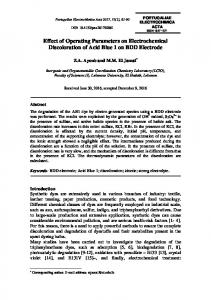
C. Effects of PWM Modulator Gain Km on the Controlto-output Voltage Transfer Function The PWM modulator gain is generally modeled as the same as that with VMC [3]. This has been experimentally verified to be valid under the assumption of negligible inductor ripple contents at the output of the current amplifier in the current loop [6]. Ways to improve modeling of the PWM modulator gain are reported in [4][5]. However, what has not been studied is how this parameter affects the ACMC Buck converter small-signal dynamics. With the expressions of the control-to-output voltage transfer function in either its concise form (4) or expanded form (5), it is difficult to identify and quantify its unique role which it plays in the transfer function. To better understand its effect on the ACMC Buck converter small-signal dynamics, Equation (6) is solved numerically with the modulator gain varied from 0.25 to 2.0 while the converter input voltage and loading are set at 12 V and 15 A, respectively. Fig. 5 illustrates how the four poles of (6) migrate and regroup as Km is varied. With an initial value of Km = 0.25, all the four poles are lying on the real axis at locations marked as “Start”. As Km increases, s1 stays essentially at the same location, which implies that effect of Km on this pole is minimal, while the frequencies of s2 and s4 decrease, and the frequency of s3 increases. As the value of Km rises further,
The above phenomenon can be adequately modeled by (16) through (19), which predict that Km affects mainly the high-frequency portion of the control-tooutput voltage transfer function represented by the second order term in (16). As Km increases, values of both the resonant frequency and quality factor rise. Additional studies showed that the relationship between the resonant frequency ω2, the quality factor Q2 of the second order term in (16) and Km were modeled well with simple square root functions given by (18)-(19). The analytical expressions (11) and (17) to (19) can be used to calculate approximate locations of the poles as they migrate and re-group in the left half of the complex plane when the value of Km changes. The two identical poles s3 and s4 at Point X2 can be approximately evaluated by using the second order term in (16). It follows that
s3 , s4 s p 3 , s p 4
n 2 2Qn 2
n 2 (
1 2Qn 2
)2 1
.
(24)
Under the condition of critical damping, the two identical real poles are
s3 s4 s p3 s p 4
n 2 2Qn 2
sp 2
(C C ) 1 1 2
2 R2 (C1C2 ) .
(25)
Thus, the frequency of the two identical poles at Point X2 is approximately equal to half the high-frequency pole, sp, of the current loop compensator. This value remains unchanged even when s3 and s4 become a pair of complex conjugates since their real parts do not depend on the value of Km. Fig. 6 shows the calculated effects of Km on the control-to-output voltage transfer function. As predicted by (18)-(19), the Bode plots clearly illustrate increasing resonance at high frequencies as Km rises.
0 50
-20 -40
30 -80
Phase Km = 0.25
-10
-100
Phase with Km increasing
-120
Phase (degs)
Gain (dB)
-60 10
-140
-30
Gain Km = 0.25
Gain with Km increasing
-160
-50
-180 10
100
1000
10000 Frequency (Hz)
100000
1000000
Fig. 6. Predicted effects of Km on the control-to-output voltage transfer function. Km varies from 0.25 to 2 with 0.5 increment. Input voltage is 12 V and loading is 15 A.
A similar analysis can be performed with the converter running at a high duty cycle. With the input voltage of 5 V and loading of 15 A, Fig. 7 illustrates how the four poles migrate and regroup as the value of Km changes from 0.25 to 2.0. The initial four poles contain two real poles and two complex conjugate poles as predicted by (10). As the value of Km increases, the quality factor, Q2 ≈ Qn2, decreases according to (13). Hence, s2 and s3 move rapidly toward the real axis and coincide at Point X1 when the value of Km becomes sufficiently large. Then, a similar pole movement pattern as in the low duty cycle operation case follows afterwards. It can be shown from the second term of (10) that under the condition of critical damping, the two real poles s2 and s3 intersecting at Point X1 can be estimated by
s2 s3 s p 2 s p 3
c 2
(26)
.
Therefore, the frequency of the two real poles at Point X1 is approximately equal to half the current loop gain crossover frequency given by (20). jω s4 End
The arrows indicate the directions of how the four poles migrate as Km increases from low to high values
Start s2
Two identical pole locations Start s4
Start End
End x1
x2
sz1
Essentially remains at the same location as Km varies
End
s2
sz2
s1
Re 0
s3 Start
s3
Fig. 7. Illustration of pole migration and regrouping as Km increases from 0.25 to 2.0. Input voltage is 5 V and loading is 15 A.
of (6) migrate and regroup as the gain increases from 0.274 to 10. Similar to the previous case in Fig. 7 when the value of the gain is low, Equation (6) contains two real poles, s1 and s4 and two complex conjugate poles, s2 and s3. As the gain increases, the magnitudes of the real parts of s2 and s3 become larger while the imaginary parts decrease until the two become real poles, coinciding at Point X1. As s2 and s3 move toward Point X1, the frequency of s4 decreases, and s1 stays nearly at its “Start” point. At the end, the transfer function contains two real poles, s1 and s2, as well as two high-frequency complex conjugate poles, s3 and s4, all of which can be approximately calculated by employing (11) and (17)(19). jω s4 The arrows indicate the directions of how the four poles migrate as the gain (R2/R1) increases from low to high values
End
Essentially remains Start at the same location as R2/R1 gain varies
s2
Two identical pole locations
Start End
Start s4
x1
sz2 Start
x2
sz2 moves to the left as R2/R1 increases
sz1
s2 sz2 End End
The trajectory is close to being a semi-cycle
End
s1
Re 0
Start s3
s3
Fig. 8. Illustration of the pole migration and regrouping as the current loop gain R2/R1 increases.
Unlike the previous case shown in Fig. 7 in which the real parts of s3 and s4 in (24) remain unchanged as the value of the gain gets larger, the real parts of s3 and s4 do become progressively smaller, suggesting less and less damping of this second order term. This observation is confirmed with the measurement data provided in Fig. 9 which illustrates predicted and measured Bode plots showing effects of the gain on the control-to-output voltage transfer function with R2/R1 = 2.74 (R2 = 4.99 kΩ), 6.81 (R2 = 12.4 kΩ) and 10 (R2 =18.2 kΩ), respectively. The input voltage is 12 V, and loading is 7.5 A. When the gain is equal to or larger than 2.74, it affects mainly the transfer function in high frequencies. There is a noticeable increase in resonance near 180 kHz as the gain rises. This observed behavior can be regarded as the interaction between the converter inductor L and the capacitor C1 in the current loop compensator. As can be seen from (18)-(19), when the value of R2 increases, the quality factor, Q2 ≈ Qn2, rises linearly with it and the resonant frequency, ω2≈ωn2, remains unchanged. The calculated resonant frequency and quality factor are:
D. Effects of Current Loop Gain R2/R1 on the Control-tooutput Voltage Transfer Function
2 n 2
Published papers focus on the effects of the midfrequency gain R2/R1 on the ACMC Buck converter current loop [1], [3]. It is demonstrated in this paper that this gain also has dramatic effects on the control-tooutput voltage transfer function. Fig. 8 shows how poles
Q2 Qn 2
Rs KmVg R1 R2C2 (C1 C2 )
1 LC1
179.7kHz
Rs K mVg R1
C1 L
1.97.
The measured resonant frequency is roughly 170.0 kHz.
E. Effects of Input Voltage on the Control-to-output Voltage Transfer Function
0 90 70
-40
Phase with R2/R1 increasing
10
-120
-10 -160 Gain with R2/R1 increasing
-50
-200 10
100
1000
10000
100000
1000000
Frequency (Hz)
Fig. 9. Predicted (solid lines) and measured (dotted lines) Bode plots showing effects of current loop gain R2/R1 on the control-to-output voltage transfer function with R2/R1 = 2.74, 6.81 and 10, respectively. Input voltage is 12 V, and loading is 7.5 A.
When the mid-frequency current loop gain is very low, this resonance is shifted to mid frequencies as can be seen in Fig. 10, which corresponds to the gain of 0.274 with R2=0.499 kΩ. The Bode plot in Fig. 10 resembles the PCMC Bode plot rather closely at low frequencies with a dominant pole located approximately at 175 Hz. On the other hand, it also looks remarkably similar to VMC with a second order resonance at around 30 kHz. This type of PCMC-and-VMC-combined Bode plot characteristic is reported in [4]. However, the paper does not provide an explanation to identify the true cause of this unique characteristic for the ACMC Buck converter. 40
200
30
150
20
0 -50 Phase with R2/R1 = 0.274
x2
s4
s3
sz1 s2
End
Start End
s2 sz2
s1
Re 0
End
Fig. 11. Illustration of pole migration and regrouping as the input voltage changes from 5 V to 24 V. Resonance occurs at high input voltages with the converter running at a low duty cycle.
-100
-30 -40 -50 100
Start
Start
Essentially remains at the same location as Vin varies
Phase (degs)
Gain (dB)
0 -10
10
Start
The arrows indicate the directions of how the four poles migrate as input voltage increases from low to high values
s3 50
-20
End
100
Gain with R2/R1 = 0.274
10
jω s4
1000
10000 Frequency (Hz)
100000
-150
50
-200
40 30
1000000
Fig. 10. Predicted (solid line) and measured (dotted line) Bode plots of the control-to-output voltage transfer function with R2= 0.499 kΩ, R2/R1 = 0.274, 12 V input voltage and 7.5 A load.
With an ultra low current loop gain, the equation representing the converter is given by the simplified ACMC small-signal model (10). Using (12) and (13), we estimate the resonant frequency and the quality factor to be 30.82 kHz and 4.78, respectively. The measured resonant frequency is 28.18 kHz. It is conceivable that the observed resonance results from the interaction between the converter inductor L and the two capacitors, C1 and C2, in the current loop compensator with C2 being the main contributor since its value is generally much larger than that of C1. The above analysis has demonstrated that when the current loop gain is either small or large, the resultant second order resonance has a frequency-shifting property. In neither case, the resonant frequency is fixed at half the switching frequency of 250 kHz.
0
-36
20 10
-72 Phase with input voltage increasing from 5V to 24V
0
-10
Phase with 5V input voltage
-20 -30
-108 Gain with 5V input voltage
-144
Gain with input voltage increasing from 5V to 24V
-40
Phase (degs)
-30
Pole migration and regrouping of the control-to-output voltage transfer function can also take place when the input voltage (an operating parameter) changes. Fig. 11 shows a typical pole movement pattern as the input voltage is varied from 5 V to 24 V, which corresponds to a duty cycle variation from 0.68 to 0.14. Loading is fixed at 7.5 A. Fig. 11 indicates that the pole migration and regrouping under this operating condition is very similar to that illustrated in Fig. 5. Therefore, the same reasoning and explanation do apply here. Pole movement under the condition of duty cycle changes is discussed briefly in [6], and the results reported in this paper confirm the author’s observations. Fig. 12 illustrates Bode plots of the predicted and measured control-to-output voltage transfer function as the input voltage varies. Experimental results in Fig. 12 confirm the analysis represented by Fig. 11.
Gain (dB)
Gain (dB)
-80 30
Phase (degs)
50
-50
-180 10
100
1000
10000 Frequency (Hz)
100000
1000000
Fig. 12. Predicted (solid lines) and measured (dotted lines) Bode plots showing effects of input voltage variation from 5 V to 24 V on the control-to-output voltage transfer function.
To demonstrate the usefulness of the simplified expressions (10) and (16) to model the observed phenomenon, TABLE IV tabulates calculated poles, zeros, resonant frequencies and quality factors with a few selected input voltage values.
TABLE IV CALCULATIONS OF POLES, ZEROS, RESONANT FREQUENCIES, AND QUALITY FACTORS UNDER DIFFERENT INPUT VOLTAGES Pole, zero, ω and Q factor fp1(Hz) fz2(kHz) sp2 or fp2(kHz) sp3 fesr(kHz) fn1(kHz) Qn1 fn2(kHz) Qn2 fp4 (kHz) or sp4 fz3(MHz)
51 168.31 7.03 -19.88+ 1.23i -19.881.23i 15.92 19.92 0.49 x x 328.6 1.20
Input Voltage (V) 12 18
24
172.58 7.03 9.84
173.63 7.03 9.84
174.16 7.03 9.84
-166.873.89i 15.92 x x 179.7 0.55 -166.8+ 73.89i 1.20
-166.8148.6i 15.92 x x 220.0 0.67 -166.8+ 148.6i 1.20
-166.8196.7i 15.92 x x 254.0 0.77 -166.8+ 196.7i 1.20
1. Poles, zeros, resonant frequency, and quality factor are calculated by using (11)-(14) for 5 V input voltage. The rest are calculated by using (17)-(19) for other input voltages.
The above calculations clearly describe the measured data in Fig. 12. For practical design purposes, Equation (16) can be further simplified by noting that the zero, sz2, in (7) and the pole, sp2 in (17) generally lie in the vicinity of each other in the mid-frequency range with fz2 < fp2. Therefore, they effectively cancel each other. Moreover, sz3, should be ignored since it is usually located well beyond half or even greater than the converter switching frequency. Equation (16) becomes Tp ( s )
(1rcCs ) RL Rs (1 s )(1 s s2 ) s p1 n 2Qn 2 2 .
(27)
n2
This is the minimum order control-to-output voltage transfer function for the ACMC Buck converter operating under a low duty cycle. Equation (27) distinctly illustrates similarities and differences between ACMC and PCMC with or without considering sampling effect [9]-[11]. IV. MORE DISCUSSIONS In the previous Section, various properties of ACMC Buck converters are discussed as the circuit and operating parameters change. Parameter effects are highlighted in this Section for other topologies. A. Parameter Effects on the Current Loop and Controlto-output Voltage Transfer Functions for the BuckBoost Converter Parameter effects can be sufficiently investigated by using the simplified ACMC model for the Buck-Boost converter [8]. Since the equations describing the smallsignal dynamic behavior for this topology are very similar to those for the Buck topology, it is easy to show that poles are equally sensitive to parameter variations, and very comparable results and conclusions are expected to be obtained.
B. Parameter Effects on the Current Loop and Controlto-output Voltage Transfer Functions for the Boost Converter For Boost converters, it is shown in [8] that the current loop gain crossover frequency does not depend on the input voltage. This is a unique advantage for the ACMC Boost converter to be used for Power Factor Correction (PFC) rectifiers. Moreover, poles, resonant frequencies, and quality factors are also independent of the input voltage. Once the converter is designed, input voltage influences only the DC gain of the control-tooutput voltage transfer function. Other parameter effects are very similar to these for the other two topologies. V. CONCLUSIONS A detailed and in-depth study of effects of converter circuit and operating parameters on the small-signal dynamics of ACMC Buck converters has been presented. Despite some similarities between ACMC and PCMC control schemes, the study reveals some rather interesting properties and insight into ACMC that are not present for PCMC. Understanding these sole characteristics enables us to develop more effective design strategies on an analytical basis. REFERENCES L. H. Dixon, “Average current-mode control of switching power supplies,” Unitrode (Texas Instruments) Power Supply Design Seminar Manual, 1990. [2] C. Sun, B. Lehman and J. Sun, “Ripple effects on smallsignal models in average current mode control,” Conference Proc. of IEEE APEC 2000, Vol. 2, pp. 818823. [3] J. Sun, R. Bass, “Modeling and practical design issues for average current control,” Conference Proc. of IEEE APEC 1999, Vol. 2, pp. 980-986. [4] T. Suntio, J. Lempinen, I. Gadoura, K. Zenger, “Dynamic effects of inductor current ripple in average current mode control,” Conference Proc. of IEEE PESC 2001, pp. 1259 – 1264. [5] W. Tang, F. Lee and R. B. Ridley, “Small-signal modeling of average current-mode control,” IEEE Transaction on Power Electronics, Vol. 8, No. 2, pp. 112119, 1993. [6] P. Cooke, “Modeling average current mode control,” Conference Proc. of IEEE APEC 2000, Vol. 1, pp. 256262. [7] R. Li, “Modeling average-current-mode-controlled multiphase Buck converters,” Conference Proc. of IEEE PECS 2008, pp. 3299-3305. [8] R. Li, T. O’Brien, J. Lee, J. Beecroft, “A Unified small signal analysis of DC-DC converters with average current mode control,” Conference Proc. of IEEE ECCE 2009, pp. 647-654. [9] R. W. Erickson, D. Maksimovic, Fundamentals of Power Electronics, 2nd Edition, Kluwer Academic Publishers, 2001. [10] R. D. Middlebrook, “Topics in multiple-loop regulators and current-mode programming,” IEEE Transactions on Power Electronics, Vol. 2, No. 2, pp. 109-124, 1987. [11] R. Ridley, “A new, continuous-time model for currentmode control,” IEEE Transactions on Power Electronics, Vol. 6, No. 2, pp. 271-280, 1991. [1]