Efficient computation of PCA with SVD in SQL - Semantic Scholar

Efficient computation of PCA with SVD in SQL Mario Navas

Carlos Ordonez

University of Houston Dept. of Computer Science Houston, TX 77204, USA

University of Houston Dept. of Computer Science Houston, TX 77204, USA

ABSTRACT PCA is one of the most common dimensionality reduction techniques with broad applications in data mining, statistics and signal processing. In this work we study how to leverage a DBMS computing capabilities to solve PCA. We propose a solution that combines a summarization of the data set with the correlation or covariance matrix and then solve PCA with Singular Value Decomposition (SVD). Deriving the summary matrices allow analyzing large data sets since they can be computed in a single pass. Solving SVD without external libraries proves to be a challenge to compute in SQL. We introduce two solutions: one based in SQL queries and a second one based on User-Defined Functions. Experimental evaluation shows our method can solve larger problems in less time than external statistical packages.

Categories and Subject Descriptors G.1.3 [Mathematics of Computing]: Numerical Linear Algebra—Singular value decomposition; G.3 [Probability and Statistics]: Multivariate statistics; H.2.4 [Database Management]: Systems—Relational databases; H.2.8 [Database Management]: Database Applications—Data mining

General Terms Algorithms, Performance, Theory

Keywords PCA, SVD, SQL, DBMS

1.

INTRODUCTION

Principal component analysis or PCA is a popular technique in statistics and data mining for dimensionality reduction. It is a valuable tool to reveal hidden patterns, compress and extract relevant information from complex data sets. Several applications for image processing [6], data compression [3], pattern recognition [23], clustering [5], classification

Permission to make digital or hard copies of all or part of this work for personal or classroom use is granted without fee provided that copies are not made or distributed for profit or commercial advantage and that copies bear this notice and the full citation on the first page. To copy otherwise, to republish, to post on servers or to redistribute to lists, requires prior specific permission and/or a fee. DMMT’09, June 28, 2009, Paris. Copyright 2009 ACM 978-1-60558-673-1/06/09 ...$10.00.

[9] and time series prediction [22] have developed over time around PCA. By successfully applying linear algebra, PCA finds the optimal linear scheme, in sense of least square errors, to reduce dimensions of a data set. Traditionally PCA is computed by exporting data as flat files compatible with statistical tool specifications. Since the complete data set is uploaded into main memory, handling large amount of information is a major concern for analysis. Few proposals have taken into account the integration of statistical methods into the DBMS, due to its limitations to perform complex matrix and vector operations. Constructing statistical models efficiently inside the DBMS is a key factor to add data mining capabilities into the DBMS [16]. Previous research has used user defined functions (UDFs) to enrich the DBMS with PCA [20]. We have extended past work by successfully implementing all steps participating in PCA with SQL statements. Compared with UDFs, SQL is portable among DBMS providers. Also the query optimizer manipulates disc and memory I/O operations to run without data size limitations. Additionally this article includes a comprehensive analysis of implementation alternatives to optimize execution time without affecting correctness of the results. Our focus is to deal with large amount of data and overcome limitations of statistical applications. The article is organized as follows. Section 2 presents definitions. Section 3 presents our contributions, how PCA is solved inside the DBMS with SQL statements, along with some implementation choices. Section 4 presents experiments comparing different methods of correlation analysis, SVD implementation inside and outside the DBMS, SVD optimizations to reduce execution time. Section 5 includes related work. In Section 6 we present conlusions and future work.

2.

PRELIMINARIES

In this section we explain PCA, the relation with SVD and the algorithm to solve the eigen-problem. The initial step is to compute the correlation matrix used as input for PCA. Next, we explain the fundamentals of dimensionality reduction, together with the connection to the eigen-problem. We show how the QR algorithm performs the Householder tridiagonalization of the correlation matrix and iteratively the QR decomposition, returning the principal components.

2.1

Definitions

Let X = {x1 , ..., xn } be the input data with n points, where each point has d dimensions. X is a d × n matrix, where the point xi is represented by a column vector (equiv-

alent to a d × 1 matrix). We use the subscripts i and j to indicate position of a value in a matrix, thus xij is the value at the row i and the column j of X. The subscripts k and s are used to identify the number of the current execution step. Matrix transposition is denoted by T , likewise norm of a vector as ||xi ||. The matrix Q, from the summary matrices L and Q, is not to be confused with Q from the QR decomposition. The storage of the data set X and table definitions in a DBMS, can be found in Section 3.1.

2.2

Data Preprocessing

In order to perform PCA, the first step is either to compute the covariance or the correlation matrix of the input data set with data centered on the mean (substracting µ). The covariance matrix of X is a d × d matrix with measures of how the dimensions change together and a main diagonal of variances. It is defined as follows: CX =

1 XX T n−1

(1)

Correlation coefficients are more desirable because they indicate the strength and direction of the linear relationship between two variables in the range [−1, 1]. Therefore, a correlation matrix is normalized, symmetric d×d and populated with the degree of correlation among dimensions. Such matrix can be calculated using the summary matrices: L and Q [16]. Let L (see Equation 2) be a column vector d×1 with the linear sum of points with elements of the form Li where i = 1, 2, .., d. At the same time, let Q (see Equation 3) be the quadratic sum of points, in the sense that the d × d matrix with values Qij is the sum of the cross-products of each point with its transpose. These summary matrices allow us to compute several statistical techniques efficiently, due to its small size compared to X when d )

Figure 3: QR Algorithm Implementation. For the QR algorithm (see Figure 3), the number of steps required to reach a solution depends on an error criteria , which is computed out of the diagonal elements of Ak . The loop starts with k = 0 and at each step Ak−1 = Qk Rk

is calculated using the QR Factorization (see Figure 4), it becomes a nested loop of the iterative QR algorithm [21]; initially Qk = Ak−1 = {v0 , v1 , ..., vd }, and the values of Rk are given by Rk = {ri,j }. Notice that Householder is finished before the QR algorithm starts, therefore their step counters k are not the same. 1 2 3 4 5 6 7 8

For i = 1 to d rii = ||vi || vi = vi /rii For j = i + 1 to d rij = vi · vj vj = vj − rij vi End End

Figure 4: QR Factorization Implementation. After completion of the main steps the eigenvalues need to be positive. Thus for every negative value ai,i in the diagonal of A, ai,i = −ai,i and uj,i = −uj,i ; where j = 1, 2, ..., d. Finally, E 2 = {ai,i } and E −1 = { √a1i,i }. In the next sections the detailed implementation of the main steps of SVD with SQL statements as well as the technical overview of the coding inside the database is exposed.

3.

SVD IN SQL

In this section we explain the techniques for matrix multiplication, matrix transposition, along with the fundamental operations used in our SQL implementation. The detailed explanation of the steps of the algorithm can be found in Section 2.4, our SQL implements such definition. Further analysis of space, I/O and complexity of our SQL queries is performed for each step of the algorithm.

3.1

Table Definitions

In order to represent matrices as tables in a DBMS, we can define the columns as dimensions and rows as records. For the input matrix X the storage table, tX, contains the attributes {X1 , X2 , ..., Xd }. This matrix is used to compute the input correlation matrix of the algorithm in order to find its decomposition (see Section 2.4). Matrix operations, such as multiplication, can be performed with this representation by pivoting the left or the right operator to pair rows of one matrix with columns in the other and obtain the resulting table with an AGGREGATE statement. Another way to store matrices is vertically [14]. Vertical layout matrices {i, j, val} are implemented to perform multiplications and other matrix operations needed to solve the eigen-problem. There is no need to pivot multiplying matrices and it is a very convenient method to implement operations in the algorithm steps. For instance, the multiplication of a pair of matrices A and B, which are stored with vertical layout, could be done in one SQL statement with one JOIN condition and an AGGREGATE function. Moreover trivial values are not required to be stored, such as, zero values of an sparse matrix or values which can be computed from or are equal to other elements in the same matrix. We also exploit the fact that for a multiplication result, the element {i, j, val} can only exist if there exists at least one element {i, k, val}} for the left operator and at least one match {k, j, val} for the right operator. This is

used to avoid unnecessary pairing and to reduce the number of values involved in the AGGREGATE. Notice that the computation of a value during multiplication of two d × d matrices will have the cost of joining (pairing), a product operation and an aggregation of d values. Pursuing to alleviate the computation time of JOINs, which are the most expensive computation in SQL, our code uses constraints that cut down the unnecessary records during operations. For PCA (see Section 2.4), the resulting principal components and their associated variances will be stored on tables tU and tA respectively. Table 1 has the summary of tables used for storage and their scope. In the QR factorization the tables tQ and tR have an extenal scope in the sence that they exist outside the loop, then the QR algorithm uses them to compute new values for the tables tA and tU. Therefore, tables tQ and tR are not needed beyond the scope of an iteration of the QR algorithm. Thus, even though names overlap for local table definitions, the only common tables between steps are tU and tA. Table 1: Summary of Step Global Correlation tX, tA Householder tA, tU QR algorithm tA, tU

tables in SQL. Local tL, tQ tW, tP, tH, tT tQ , tR, tT

Further optimization is done to take advantage of SQL when performing Householder and QR factorization. The details about how SQL statements and tables map the steps of the algorithm will be shown in the next sections.

3.2

Correlation Computation

The computation of n, L, Q are sufficient statistics to compute the correlation matrix (see Section 2.2). When the data set is in vertical layout, the table stores one correlation value per row as {i, j, ρij }. Since the matrix is symmetric, it is sufficient compute a triangular matrix with the number of rows of the resulting matrix equal to the total number of correlation pairs (d(d+1)/2). The number of INSERT state. Retrieving ments to compute n is 1, L is d and Q is d(d+1) 2 every singular value with an AGGREGATE function involving a scan of tX, can be avoided with a more conservative approach [15, 17]. It is a single SELECT with 1 + d + d(d+1) 2 AGGREGATE statements using tX. SELECT sum(1.0) AS n ,sum(X1 ),sum(X2 )...,sum(Xd ) /*L*/ ,sum(X1 ∗ X1 ) /*Q*/ ,sum(X2 ∗ X1 ),sum(X2 ∗ X2 ) . . . ,sum(Xn ∗ X1 ),sum(Xn ∗ X2 ),...,sum(Xn ∗ Xn ) FROM tX; The resulting query is stored on a temporary table and then inserted with vertical layout in the tables tL and tQ. Finally, the values of the correlation matrix are computed from the summary matrices without performing more scans on the original data set. The final table storing the correlation coefficients, tA, has 3 columns and (d(d + 1)/2) records.

3.3

Householder Transformation

Our implementation of Householder in SQL uses vertical matrices to exploit the storage of sparse matrices, and also other optimizations of operations. The resulting tables tA storing Ak−2 and tV storing Vd−2 are obtained using only INSERT statements. We use the auxiliary table tH to store the part of the matrix Ak that will be rotated during following iterations and the table tT to store the sub matrix of Vk that will continue to be involved in further operations. Such implementation is possible as the matrix Pk is composed of a diagonal identity matrix of k elements and a square matrix starting at the position (k + 1, k + 1). Consequently, the values of Pk that are not trivial have the form {[k + 1, d], [k + 1, d], val} and stored on the table tP. During each iteration instances of the tables tH, tT, tP and tW are computed, along with the variables alpha and r. Meanwhile the values inserted in tA and tV are never updated. First tH is instantiated with the input correlation matrix. Values for the variables alpha and r are computed with SELECT and AGGREGATE statements over the table tH. The table tW, storing the vector w, has the form {[k + 1, d], val}, not including zero values. Since tW has d − k − 1 values and the table tP is symetric, only the upper or bottom diagonal matrix is stored. tP has size ((d − k + 1)(d − k + 2)/2) + 1, which is calculated with two statements: one to insert the record {k, k, 1}, necessary to include the column and the row k in our operation results, and other to compute the difference between I and the cross product of the values in tW. As shown in Figure 5, during iteration k only the sub 

a a 0 ... 0 a a a . . . 0  0 a a ... 0  ..  .. .. .. . . . . . . .  0 0 0 . . . a k,k  0 0 0 . . . ak+1,k  0 0 0 . . . 0  . . . . .. ..  .. .. .. . 0 0 0 ... 0

0 0 0 .. . ak,k+1 h h .. . h

0 0 0 .. . 0 h h .. . h

 ... 0 . . . 0  . . . 0  .. ..  . .  . . . 0  . . . h  . . . h  ..  .. . . ... h

Figure 5: Storage of matrix A at step k, in tA:{i, j, aij } and tH:{i, j, hij }. matrix {[k, d], [k, d], value)} changes from Ak−1 to Ak . The rotation tP of tH from the previous iteration with the form {[k, d], [k, d], val} has the elements ak,k , ak+1,k and ak,k+1 of the final matrix An−2 to be stored on tA, also the sub matrix {[k + 1, d], [k + 1, d], val} to be the new instance of tH. The matrices stored on tH, tP, tA are symetric, therefore only the triangular upper or lower matrix is stored, moreover computations are cut down only for such values. Nevertheless, it is important to include the values not stored at the moment of doing the aggregations of matrix multiplications. Since Pk is applied as a transformation at the right side of Uk−1 , it only alters values for the columns of the range [k + 1, d]. At each iteration a new instance for the table tT is generated, which stores a sub matrix of Uk (see Figure 6) with tuples of the form {[2, d], [k + 2, d], val} obtained from the multiplication between the instance of tT at it-



1 0  0   .. .  0  0  .  ..

0 0 u u u u .. .. . . u u u u .. .. . . 0 u u

... 0 ... u2,k+1 ... u3,k+1 .. .. . . . . . uk+1,k+1 . . . uk+2,k+1 .. .. . . ... ud,k+1

0 t t .. . t t .. . t

 0 ... 0 t . . . t  t . . . t  .. .. ..  . . .  t . . . t  t . . . t  .. . . ..  . . . t ... t

Finally, we have that no UPDATE statement is required to obtain Qk and Rk . Which is very close from the database point of view. And the only table that needs to be recomputed per iteration is tT. 

q q  0   .. .  0  0  0  0  .  .. 0

Figure 6: Storage of matrix U at step k, in tU:{i, j, uij } and tT:{i, j, tij }. eration k − 1 and the values in tP . The remaining tuples {[2, d], k + 1, val} are to be inserted in tU.

3.4

QR Factorization

As described in Section 2.4, the QR factorization is iteratively called by the QR algorithm. In each step, a row of Rk is computed and the columns vj of Qk where j ≥ i are modified. As shown in Figure 7, Qk is stored on tT and tQ. The table tT is initiated with a copy of the input matrix Ak−1 . For the step i, vi and ri,i are computed, both to be inserted in tQ and tR respectively. Vertical matrix representation allows us to compute the internal loop with three SQL statements. One for the column of Rk {[i], [i, d], val}, with the AGGREGATE of the JOIN between vi and tT on the row value. The second to compute the new instance of tT, with a join between the previous tT, vi and tR. Notice that this matching will result on records of the form {[1, i + 1], [i + 1, d], val}, consequently the remaining {[i + 2, d], [i + 1, d], val} from the old tT is inserted with a third statement. Given @i = i and @r = ri,i , the SQL is as follows, /*New values for tQ*/ INSERT INTO tQ SELECT tT.i, tT.j, tT.val / @r FROM tT WHERE tT.j = @i; /*New values for tR*/ INSERT INTO tR SELECT @i, @i, @r UNION ALL SELECT tQ.j, tT.j, sum(tQ.val * tT.val) FROM tQ,tT WHERE tQ.j=@i AND tT.j>@i AND tQ.i=tT.i GROUP BY tQ.j, tT.j; /*New instance of tT*/ INSERT INTO new_tT SELECT tT.i, tT.j, tT.val - tQ.val * tR.val FROM tQ, tT, tR WHERE tT.j>@i AND tQ.j=@i AND tR.i=@i AND tR.j=tT.j AND tQ.i=tT.i UNION ALL SELECT i, j, val FROM tT WHERE tT.j>@i and tT.i>@i+1

q q q .. . 0 0 0 0 .. . 0

q q q .. . 0 0 0 0 .. . 0

. . . q1,i . . . q2,i . . . q3,i .. .. . . . . . qi,i . . . qi+1 ... 0 ... 0 .. .. . . ... 0

t t t .. . t t t 0 .. . 0

t t t .. . t t t t .. . 0

t t t .. . t t t t .. . 0

... ... ... .. . ... ... ... ... .. . ...

 t t  t  ..  .  t  t  t  t  ..  . t

Figure 7: Storage of matrix Qk at step i, in tQ:{i, j, qij } and tT:{i, j, tij }.

3.5

QR Algorithm

During each iteration of the QR algorithm, there is a QR factorization, two matrix multiplications and an error computation. Since the convergence iteration is not known beforehand, new solution tables tU and tA are computed each stage. The SQL for QR factorization was explained in Section 3.4. As for the multiplications, only optimization of the computation Ak is feasible. Since Ak is a tridiagonal symetric matrix, the SQL is constrained to calculate the main and one of side diagonals of the multiplication between the matrices in the tables tR and tQ, result to be stored on tA. The table tU with the value of Uk is computed with a query of the previous instance of tU and tQ. A value for the variable error is computed with a SELECT of the maximum difference of the diagonal elements between the tables storing Ak−1 and Ak . Finally, the loop will conclude when the value of the error is less or equal the parameter .

3.6

Implementation Alternatives

Data access and manipulation in a DBMS could be done using different tools, hence, PCA is not restricted to SQL statements. Here we explain how external libraries, UDFs and Database Connectivity APIs are used to implement the main steps of PCA: correlation computation and eigenvalue decomposition. Even though external libraries are specialized pieces of software that have been developed over time to optimize execution time of their algorithms, most of them are not designed to overcome memory heap constraints. Such limitation is evident when attempting to apply large data sets to these external libraries for statistical and data mining analysis [7]. APIs, like JDBC or ODBC, allow the user to access and manipule data from external programs. This collection of libraries grant data mining applications connectivity to data sources from different DBMS providers and they can be used to minimize memory usage. Database connectivity components are extremely portable, for most of them few properties need to be changed along with the driver to switch the DBMS. Since the execution speed depends on the communication channel and for security reasons, it is desirable to minimize the amount of data transmitted through the network. Other exploitable feature

of a DBMS are user defined functions or UDFs, which are compiled to be embedded into the DBMS and can be called using SQL statements. Therefore, a UDF executes inside the DBMS without delay transmitting information. On the other hand, UDFs depend on the DBMS specification, making them not portable among providers and sometimes not feasible due to access constraints. Our focus is to optimize performance of PCA computation for large data sets by minimizing memory allocation and execution time, without altering correctness of the results. So far we have explained how to perform each step of SVD with SQL statements(see Section 3). To avoid redundancy, the structural components of the other implementation alternatives besides SQL are generalized with pseudo-code. The correlation matrix can be computed with one pass over the original data set [16]. Reading one record in the table at a time, the summary matrices are computed as an aggregation. Thus, a data structure is used to store n, L and Q, where the values obtained by combining attributes of the current record are accumulated. After finished over the whole or part (sampling) of the table, the correlation matrix is generated as specified in Section 2.2. Finally, the steps for eigenvalue decomposition, given the correlation matrix as an array of two dimensions, are mapped for most programming languages [19, 4, 10]. For our experiments we use the algorithm specification in Section 2.4.

3.7

Time and Space complexity

For the computation of the summary matrices L and Q, along with the covariance matrix, the complexity of operations in the algorithm (Section 3.2) are O(dn) and O(d2 ) respectively, the same complexity is shared by the SQL, Java and the UDF implementations. In the other hand, for the SVD (Section 2.4) all implementations maintain the same steps for the algorithm. However, for SQL operations, we need to take into account the complexity of cross product and joins. This problem is alleviated with reduction of records participating in computations by constraints and by not physically represent elements with predictable values. Complexity of the SVD [19] is analyzed by operation and iteration. Solving Householder is O(d3 ), with n − 2 steps of O(d2 ) each. Table 2 shows the number of operations for Java and the UDF, along with the records involved in operations for SQL. Even though each step of the QR factorization is O(d2 ) (see table 3), after completion of d steps the overall complexity is O(d3 ). Once again the representation in SQL incorporates equal or less records for operations. The QR algorithm includes matrix multiplications besides the QR factorization, preserving complexity of O(d3 ) per step. However, with the number of iterations for convergence s, the QR algorithm is O(sd3 ). In table 3 we observe that eventhough the records for U are not reduced in SQL, only the elements on the three diagonals of A are computed. As for the implementation alternatives to SQL, space reTable 2: Householder I/O per step. Matrix UDF & Java SQL A

(d+1)(d) 2

(d−k+2)(d−k+1) 2

U

d2

(d − k + 1)2

quirements are static. Operations of matrices are done by changing values already allocated in memory. In SQL the space requirements are closely related to the number of records used in operations or query statements. Therefore, tables in Householder and the QR factorization reduce on size when the step counter increases. Reducing the numerosity of records taking part in the join statements, improves the execution speed of this approach when compared to the counter scenario were every single value is computed for each step of the algorithm.

Table 3: QR algorithm I/O per iteration. Matrix UDF & Java SQL Qk

Pd

A

d×d

2d − 1

U

d×d

d×d

i=1

d(d − i) + d

Pd

i=1

i(d − i) + d

4. EXPERIMENTAL EVALUATION In this section we present the experimental evaluation on SQL Server DBMS. The server had an Intel Dual Core CPU, 2.6GHz, 4GB of memory and 1TB on disk. The DBMS ran under the Windows XP operating system and has implementations of the UDFs compiled. We also used a workstation with a 1.6 GHz CPU, 256 MB of main memory and 40GB on disk with JDBC connection, a SQL script generator, an implementation of SVD, JAMA and the R application for comparison purposes. We implemented three UDFs: one to compute the correlation matrix, a second to compute the SVD given a matrix and a third that computes the correlation matrix together with its SVD decomposition to return the principal components of the given table. Our optimizations combine UDFs and SQL to improve execution time. Likewise, the optimizations are also implemented with JDBC by executing some operations inside the DBMS with SQL statements and others in the workstation (see Section 3.6). For R, all the data sets were transformed into flat files, the time of exportation was not taken into account during speed measurements. JAMA has a JDBC connection to access data in the DBMS, therefore measurements include time taken to import data. We used three real data sets from the UCI Machine Learning Repository. This information comes from different backgrounds which require dimensionality reduction. The first data set contains general information on Internet users with a combination of categorical and numerical data(n=10000, d=72). A second data set is of cartographic variables for forest cover type prediction of 30 × 30 meter cells (n=100000, d=54). The last data set is of US Census Data with numeric and categorical attributes (n=100000, d=62). We varied the number of dimensions d for time performance comparisons and to test scalability. Since the results are numerical approximations, we use the maximum expected relative error δ of the most representative eigenvalue as measure of precision. Notice that the only parameter for execution is the convergence criteria  which can be modified to warranty any desired expected maximum error. The external Java package JAMA (A Java Matrix Package) and R do not

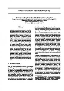
Figure 8: PCA with SQL relative error (δ).

require to set any parameter to compute the eigenvalue decomposition. Considering that all the implementations converge to the same direction, yet all solutions are numerical approximation, we report correctness based on the maximum error expectation. Given an input table of d × n, the resulting principal components or eigenvectors matrix will have size d × d. Finally, we have that each experiment is repeated 5 times and the average is reported.

4.1

Result Correctness

Our goal is to minimize the execution time without affecting the correctness of solutions. In Section 3, we showed the implementation of our QR algorithm (see Section 2.4) in SQL, without modifying any step or main operation. Optimizations are required not only to minimize the storage requirements of the matrices, but also to reduce accumulated error; since trivial or known zero values are cut off the operations. As expected, roundoff errors can swamp the process from the true solution. Also in SQL we are bound to work with the floating point operation precision of the DBMS. However, results show that the optimizations efficiently help to prevent accumulated roundoff and floating point operation errors. Convergence of the SQL implementation solving SVD over the US Census data set (n = 1000) is presented in Figure 8. The plot shows how the relative error of the eigenvalue diagonal rapidly decreases during the first steps of the algorithm eventually converging bellow the desired error criteria. As presented in Figure 9 the execution time of the SQL implementation quickly increases with the number of dimensions d. Since SVD operates over a d × d matrix, the eigenvalue decomposition is not affected by any change on the number of instances in the data set. We explained in Section 3.1 how the implementation reduces the number of values to be computed during each iteration to the minimum. Also how we take advantage of SQL and our matrix representation to acomodate matrix operations in such a way that only sub matrices interact during each step. Moreover, a value computed will only be used no more than two times before the table where it is contained is replaced by a new instance. However, the volatile nature of the matrices and the number of cross joins performed during every execution are not

Figure 9: PCA with SQL time.

to be avoided. The remarkable advantages of an SQL implementation is to be linearly scalable with n and not to have a memory heap limitation. Therefore, this approach can be used to compute PCA for a table of any size. Finally, more analysis needs to be done comparing the results against different external tools. From our experiments we have that our implementations and external libraries converge to the same direction, yet all the values vary on decimal places. Such analysis would focus on the impact of roundoff errors in the SQL floating point operations and how different algorithms to solve SVD perform better for certain datasets.

4.2

Implementation comparison

Based on the algorithm, the first step is to compute the correlation matrix. Table 4 shows a computation time of the correlation matrix in SQL and the time required by an external library to generate the same matrix in main memory. The JAMA package outperforms SQL for all the cases of n = 10. Since L requires d and Q a number d × (d + 1)/2 INSERT queries, it is not beneficial to use SQL when the number of records is relatively small. However, for all the cases with n ≥ 100, the advantage of executing operations inside the database is evident. The database not only overcame the memory issue, but also surpassed Java execution time. When correlation is computed vertically, the number of scans done to the original data set increases with d. For convenience we improved our vertical correlation matrix computation using one horizontal aggregation query with all the values for n, L and Q (see Section 3.2). Therefore, no more than one scan of the data is needed. The time of inserting the resulting attributes of the query, one at a time in the vertical result table, is insignificant when compared to the multiple scans of a table with a large number of rows. SQL Server limits the number of columns based on the total size of the row, which is capped at 8KB. As a result, when only using floating point columns, the maximum number of dimensions that can be computed with one scan is 42. A larger number of dimensions would require additional scans on the original table because we need to split the aggregate in order to fit the maximum row size allowed by the DBMS.

This explains why the horizontal aggregate is outperformed by the vertical aggregate when n = 10 and d ≥ 50. The UDF implementation (see Section 3.6) looks promising in comparison to the SQL when n ≤ 100, yet not enough to have faster results than JAMA if the data set is relatively small n = 10. Finally, we have that the horizontal aggregate dominates for n ≥ 100, due to DBMS optimizations to perform aggregates fast on large tables. Table 4: Correlation computation time in seconds with JAMA using JDBC (*out of memory). Vertical Horizontal n × 1000 d aggregate aggretate UDF JAMA 10 30 7 2 3 5 10 50 20 21 16 11 10 70 40 59 34 12 100 10 3 1 2 13 100 20 10 7 7 25 100 30 23 16 16 32 100 50 57 53 47 * 1000 20 >1K 33 72 * 1000 40 >1K 154 261 * Table 5 compares the execution time of SVD for our SQL and UDF implementations. They use the correlation matrix from the previous step to generate a numeric SVD decomposition. The relative error δ with respect to the most representative eigenvalue is set the same to compare speed. Since both implementations overcome the error criteria after certain number of steps s, there is no precision lost when executing operation in SQL. However, the price to pay is on the number of iterations executed. Considering that all the operations are done in main memory, it was expected for the UDF implementation to surpass SQL in speed. Notice that the time to compute the correlation matrix matrix was not taken in account during measurement. In order to optimize execution speed of PCA, we can combine the different implementations, this comparison is analyzed bellow. Table 5: SVD computation time in seconds with s iterations for convergence. n × 1000 d δ SQL s UDF s 10 30 3.76−3 92 78 1 80 10 50 3.65−3 481 146 3 115 10 70 2.92−3 978 172 5 122 100 10 3.49−5 6 34