Efficient Simulation of Example-Based Materials - Computer Graphics ...

Eurographics/ ACM SIGGRAPH Symposium on Computer Animation (2012) P. Kry and J. Lee (Editors)

Efficient Simulation of Example-Based Materials Christian Schumacher1,2

Bernhard Thomaszewski1 1 Disney

Stelian Coros1

Research Zurich

Sebastian Martin1 2 ETH

Robert Sumner1

Markus Gross1,2

Zurich

Figure 1: Different example-based materials illustrated on a set of plastically deforming thin plates. Abstract We present a new method for efficiently simulating art-directable deformable materials. We use example poses to define subspaces of desirable deformations via linear interpolation. As a central aspect of our approach, we use an incompatible representation for input and interpolated poses that allows us to interpolate between elements individually. This enables us to bypass costly reconstruction steps and we thus achieve significant performance improvements compared to previous work. As a natural continuation, we furthermore present a formulation of example-based plasticity. Finally, we extend the directability of example-based materials and explore a number of powerful control mechanisms. We demonstrate these novel concepts on a number of solid and shell animations including artistic deformation behaviors, cartoon physics, and example-based pose space dynamics.

1. Introduction Deformable materials are an essential part of animated movies, feature films and computer games since they are used to animate cloth, fleshy characters, and other non-rigid shapes. Thanks to progress in simulation and acquisition methods, the deformation behavior of many real-world materials can be reproduced in simulation with great accuracy. However, although some computer-animated materials are meant to match a real-world counterpart, many others are largely artistic in nature and should deform in a stylized fashion according to the vision of an animator. Controlling such art-directable materials is challenging since conventional models have unintuitive parameters and do not offer direct control over deformations. The recent work of Martin and colleagues [MTGG11] shows that example-based elastic materials (EBEM) are better suited for modeling artistic deformation behaviors. Instead of hand-selecting unwieldy parameters, the artist proc The Eurographics Association 2012.

vides a set of example poses that describe desirable deformations of the object. Unfortunately, the control offered by EBEM comes at a substantial computational cost since it requires solving a nonlinear optimization problem to reconstruct a consistent geometric representation of interpolated example poses. Our work targets both artistic control and efficiency by simulating example-based elastic materials using incompatible rest shapes combined with a compatible deformed configuration. We use example poses to define subspaces of desirable deformations by means of linear interpolation. As a central aspect of our approach, we linearly interpolate between individual elements which allows us to bypass expensive geometry reconstruction. This, in turn, results in a significant increase in computational efficiency compared to previous work. In addition, we extend the example-based simulation paradigm to shells, we explore the benefits of example-based plasticity and we highlight various scenar-

Schumacher et al. / Efficient Simulation of Example-Based Materials

ios where explicitly controlling the activation of the example poses is beneficial. Taken together, these contributions advance examplebased materials both in terms of artistic control and efficiency, allowing animators to better realize their artistic vision for non-rigid materials. We demonstrate results that show the power and flexibility of our method, including stylized cloth deformation, artistic control of character deformation, and cartoon physics of car crashes and plane races.

2. Related Work Simulating Deformable Materials has been a primary focus of graphics ever since the pioneering work of Terzopoulos et al. [TPBF87]. The following twenty five years have seen uncounted improvements in accuracy, speed and robustness that have converged into powerful methods for simulating deformable solids, surfaces, and curves. Since a summary of the state of the art within this limited space cannot do justice to all work, we refer to the survey paper of Nealen et al. [NMK∗ 06] and the references therein. As a central component of soft body simulations, modeling the material behavior, i.e., the relation between applied force and resulting deformation, has received a lot of attention. Although many works have addressed nonelastic materials [OBH02,BWHT07,WT08,GBB09], most applications are dominated by elastic deformations. Many existing methods rely on linear elastic material laws, which typically do not offer enough control over the deformation behavior for artistic applications. Using more elaborate models from continuum mechanics [ITF04], possibly nonlinear and datadriven [BBO∗ 09, STBG12], can be helpful when simulating real-world materials such as rubber and foam. However, artistic materials used in animations often do not have a realworld counterpart—and hand-selecting the parameters of a nonlinear material model in order to obtain a desired deformation is a virtually impossible task. Some specialized methods offer more intuitive parameters to control, e.g., the material behavior of cloth by imposing direction-dependent limits on the deformation [TPS09]. However, only few materials can be described adequately through deformation limits. Even if deformations can, to some extent, be controlled locally, it is often more desirable to prescribe the deformation behavior globally. For example, an artist might have a clear vision of how a character should deform, but translating this idea into a conventional material law is hard if not impossible. The example-based materials by Martin et al. [MTGG11] propose a practical solution to this problem that allows artists to describe the deformation behavior directly through a set of example poses. This is well aligned with the typical work-flow of artists, who routinely sculpt deformations for character animation techniques such as blend shapes or pose space deformation [LCF00]. While

the method described herein has the same motivation as [MTGG11], it is more efficient, handles example-based plasticity, and offers greater directability. Controlling Animations is necessary in most practical applications. One approach is to compute globally optimal control forces that make an object satisfy given motion objectives defined through a sparse set of key-frames [WK88, WMT06, BP08, BdSP09]. An alternative is to use local controllers that compute control forces from smaller time windows, e.g., with the size of a single time step [CMT∗ 12]. Having a high-resolution simulation track a coarse input animation can be useful for animation layout [BMWG07]. Another type of motion control can be implemented by keyframing the rest shape of a deformable character [KKA05]. Our work does not aim at controlling animations on this level; rather than having an object move along desired trajectories, our goal is to have objects deform in desired ways. Interpolating Shapes is an important problem of geometry processing. Of the numerous solutions that have been proposed (see, e.g., [ACOL00, LSLCO05, KMP07]), our work is closest related to methods that interpolate in deformation or strain space: the scheme described by Martin et al. [MTGG11] interpolates between volumetric solids using the Green strain; Winkler et al. [WDAH10] as well as Fröhlich and Botsch [FB11] interpolate between surfaces using edge lengths and dihedral angles. As a common point of strain space schemes, the interpolated configuration has to be reconstructed into geometry. Since not all strain space configurations have a geometric counterpart, the reconstruction has to be done in a least squares sense. In the context of animation [MTGG11], this requirement has lead to significant computational overhead. However, as recently shown by Coros et al. [CMT∗ 12] the reconstruction can be sidestepped by resorting to an incompatible rest shape representation—our work builds on this concept. However, whereas the method described in [CMT∗ 12] actively controls deformable characters, this work aims at controlling the deformation behavior of passive elastic materials.

3. Example-Based Materials Our method takes as input a deformable object whose equations of motion, discretized in space, are given by M¨x +

∂Wi = fext ∂x

(1)

Here, x and x¨ are the positions and accelerations of the object’s nodal degrees of freedom (DOF), M is the mass matrix, Wi = W (X, x) represents the internal potential energy, X denotes the object’s undeformed configuration, and fext stores the sum of external forces due to gravity, friction and contacts. c 2012 The Author(s)

c 2012 The Eurographics Association and Blackwell Publishing Ltd.

Schumacher et al. / Efficient Simulation of Example-Based Materials

4. Incompatible Shape Representation We start with a brief review of the interpolation scheme used in EBEM before explaining our new approach.

Figure 2: Artist-provided poses X1 and X2 specify a subset of desirable deformations. During simulation, a secondary potential energy term attracts the current deformed configuration x to Xw , its projection on the example-manifold. We represent the input poses, as well as Xw , as a disconnected set of elements, which greatly simplifies our problem formulation. Following the EBEM paradigm, we add a second elastic energy term, Wp , to (1) in order to promote user-specified internal deformations. The rest state of this energy is chosen dynamically from an example-manifold E, which is the subspace of desirable deformations spanned by a set of input example poses Xi , 1 ≤ i ≤ n. Every configuration Xw = Xw (w) ∈ E is uniquely defined by the example poses and a weight vector w = (w1 , . . . , wm ) with weight wi corresponding to Xi . The definition of the example-manifold E plays a paramount role and we introduce our approach in Sec. 4. Without loss of generality, we define the distance dE (x) of a given deformed configuration x to the example-manifold as dE (x) = min Wp (w, x) w

s.t.

Xw (w) ∈ E .

(2)

Here, Wp (w, x) = W (Xw (w), x) is used as a generalized distance measure and the minimizer Xw is the point on the example manifold that is closest to x. We refer to the operation that maps from a given x to the closest Xw as a projection. During animation, we want to always choose Xw as the projection of the current configuration x such that the internal forces generated by Wp attract x directly to the examplemanifold. In order to achieve this, we couple time integration and projection by minimizing h2 T a Ma +Wi (X, x) +Wp (w, x) − xT fext (3) 2 simultaneously for both x and w. The nodal accelerations H(x, w) =

x − xo vo − (4) h h2 are computed using the current positions as well as the positions xo and velocities vo from the previous time step. Solving this optimization problem is equivalent to performing an implicit Euler step in x, and minimizing the Wp term ensures that the resulting Xw is closest to x in the sense of (2). a=

c 2012 The Author(s)

c 2012 The Eurographics Association and Blackwell Publishing Ltd.

EBEM is based on a strain space interpolation, i.e., every interpolated configuration Ew (w) is a convex combination of the strain vectors of the input poses Ei = E(Xi ). Here, Ei are concatenations of the Green strain vectors of individual (tetrahedral) elements. Interpolated strain vectors Ew do generally not have a corresponding configuration in geometry space. Nevertheless, geometry information is needed in order to define the example potential Wp (at least for solids). Hence, the geometry Xw (w) corresponding to the interpolated configuration has to be reconstructed from the strain space configuration Ew (w). Reconstructing a compatible mesh from a given strain configuration is a nonlinear operation that does not admit a closed form solution. Therefore, the nodal coordinates of Xw have to be treated as explicit optimization parameters and the condition that Xw be in correspondence to w is enforced via a penalty term. This roughly doubles the number of DOFs and leads to a significant increase in computation time compared to an ordinary animation Our Approach is to use an incompatible representation for the example manifold, i.e., we represent both the examples Xi and the interpolated configuration Xw as sets of disconnected elements (see Fig. 2 for an illustration). Depending on the deformable model, these elements can be represented by vertex positions expressed in a rotation-free reference frame (solids) or edge lengths and dihedral angles (shells). Since the elements of the example poses Xi live in a rotationinvariant space, we can express each configuration Xw from the example-space as an element-wise linear combination of the example poses. We can thus bypass the need to reconstruct globally compatible geometry, which has a significant impact: with Xw being an explicit (linear) function of w and Xi , there is no need for introducing additional DOFs. As we show in Sec. 6, this leads to a substantial performance improvement compared to EBEM. Analysis In the EBEM formulation, the example potential Wp is zero everywhere on the manifold by construction. This ensures that deformation in the example-space is free, whereas deformation away from it is penalized. Our approach leads to a slightly different picture. When varying Xw across the example space, the minimum of Wp (Xw , x) with respect to x is zero at the examples, whereas it is nonzero for any other configuration (see Fig. 3, left). This energy landscape is a direct consequence of the fact that interpolated incompatible configurations can generally not be reconstructed into compatible geometry without introducing distortions. This gives rise to two potential concerns: (1) the energy-minimization might produce a tendency for the deformed configuration x to drift towards the examples where

Schumacher et al. / Efficient Simulation of Example-Based Materials

reference frame. In this space, element interpolation reduces to interpolation of vertex coordinates. Every vertex p j of ew can therefore be expressed as pj =

n

j

∑ wi pˆ i

(5)

i=1 j

Figure 3: Left: energy landscape on the example manifold. Right: generalized forces due to weight variation.

where pˆ i is the corresponding vertex of ei , expressed in the common reference frame. It is worth noting that, in this setting, interpolation of vertex coordinates is equivalent to interpolating co-rotated Cauchy strains. Finally, because the input example poses do not change, this reference frame needs to be computed only once as a preprocessing step. 4.1.2. Shells

Wp assumes its minimum value of zero. (2) since the minimum of Wp is not constant across the manifold, some amount of work has to be done in order to move x from one example to another, which might result in a resistance to deformation in the example-space. In order to estimate the significance of these concerns in practice, they have to be put in perspective relative to the effects resulting from the conventional potential Wi (a) pulls the deformed configuration to the rest shape, as does drift, and (b) Wi resists general non-rigid deformation, including those in the example space, as does resistance. Apart from the many animations that we created with our method, we also performed an additional experiment to isolate and quantify these effects. As discussed in Sec. 6, we found both drift and resistance to be insignificant in practice. 4.1. Application to Solids and Shells We apply our approach to common models for volumetric solids [ITF04] and thin shells [GHDS03]. Due to the different deformation measures used by these models, we handle the interpolation of solids and shells differently. 4.1.1. Solids We model three-dimensional solids using tetrahedral Finite Elements and a modified St. Venant-Kirchhoff material model as described in [MTGG11]. Evaluating this energy requires the vertex coordinates for the deformed and undeformed configurations. It is hence natural to use a positionbased representation for the elements of Xw . For every tetrahedral element e of the deformable object (in undeformed configuration), let ei be the corresponding element in the ith input example pose, and ew be the corresponding element in Xw . We first center all elements at the origin, and then extract the rotation matrix Ri between e and ei . This is accomplished by performing a polar decomposition on the deformation gradient between the two elements. Multiplying the vertex positions of ei by RTi results in all elements corresponding to e being expressed in a common

To simulate thin shells and cloth we use the discrete shell model of Grinspun et al. [GHDS03]. The elastic potential is, in this case, defined as a function of differences in edge lengths and dihedral angles between undeformed and deformed configurations. It is therefore natural to represent Xw in terms of these basic elements rather than vertex positions. As suggested by Fröhlich and Botsch [FB11], we linearly interpolate between the individual edge lengths and dihedral angles of the example poses. Again, because the interpolated configuration is only used to compute the rest state for the example potential Wp , we can bypass the global geometry reconstruction used in [FB11]. 5. Example-Based Plasticity Modeling the elastic (reversible) deformation behavior using examples has many useful applications and it would be desirable to also control plastic (persistent) deformations in a similar way. As explained in this section, our framework can be extended in a straightforward manner to support such example-based elasto-plastic materials. Our models for solids and shells measure deformations in different ways (tensors vs. scalars) such that different approaches are required for implementing plasticity. However, the underlying concept is the same: we restrict plastic deformations to the space defined by the (element-wise) interpolation of a set of input shapes. 5.1. Solid Plasticity We extend the elastic solid model of Irving et al. [ITF04] to plastic deformation using a multiplicative approach based on the decomposition of the deformation gradient F = Fe F p into elastic and plastic components. Following Bargteil et al. [BWHT07] we keep track of the plastic deformation by storing F−1 p , which simplifies the computation of the elastic deformation Fe = FF−1 p . After simulation step n, the plastic deformation for step n + 1 is computed per element using the singular value decomposition (SVD) of its elastic deformation gradient Fe,n = Un Σn VTn . The update rule is −1 ˆ −γ T F−1 p,n+1 = F p,n Vn Σn Vn

(6)

c 2012 The Author(s)

c 2012 The Eurographics Association and Blackwell Publishing Ltd.

Schumacher et al. / Efficient Simulation of Example-Based Materials

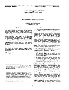
Figure 4: Different plasticity approaches illustrated on a vertically compressing cuboid (a) with a single twist example provided. Plastic deformation without examples (b), example-based plasticity with projection (c), and additional distance-dependent yield threshold (d).

where Σˆ n = det(Σn )−1/3 Σn and γ is the rate of plastic deformation. Note that this formulation ensures that plastic deformation is volume preserving since Vn is an orthonormal matrix and Σˆ n has unit determinant by definition. Following Wicke et al. [WRK∗ 10] the rate of plastic deformation is computed as γ = ν∆t

||σ||F − τ , ||σ||F

(7)

where τ is the plastic yield threshold and ||σ||F is the Frobenius norm of the Cauchy stress tensor σ. In order to obtain σ, we first compute the second Piola Kirchoff stress S=2

∂W , ∂C

The parameter τ in (7) controls how much elastic deformation is required before plastic deformation occurs. Since we want plastic deformation to occur only in the space spanned by the input examples we enforce this condition on a per-element basis. It is most convenient in this case to represent the input examples as well as interpolated configurations as sets of elemental Green strain vectors E j . For a given tetrahedron, we start by projecting its current Green strain E = 12 (C − I) onto the element’s example space. This breaks down to computing a set of weights w = (w1 , . . . , wn )T such that the projected strain (9)

j

minimizes the distance measure d = ||E − Eproj ||F . If the distance d is too large, the deformation is far away from the desired subspace and we want to discourage plastic deformation. This can be done conveniently by modifying the plastic yield criterion as τ0 = τ + ηd, where η controls the influence of d on the onset of plastic flow. c 2012 The Author(s)

c 2012 The Eurographics Association and Blackwell Publishing Ltd.

For the purpose of illustration, we ran a simple animation that emphasizes the different concepts. As shown in Fig. 4a, a cuboid is deformed by applying a compressive force along its axis. Depending on the plasticity model, different equilibrium poses result once the force has been removed (Fig.4bd). A conventional plastic material results in a bulged-out shape (Fig. 4b). Using example-based plasticity with a single twist example but without distance-dependent yield threshold leads to a twisted equilibrium pose although this deformation never occurred during compression. Finally, using the distance-dependent yield criterion leads to the desired behavior, i.e., in this case no plastic deformation.

(8)

where C = FT F is the right Cauchy Green tensor. The Cauchy stress then follows as σ = J −1 FSFT where J = det(F) [BW97].

Eproj = ∑ w j E j

While this approach encourages plastic deformation in the example space, it does not enforce this as a hard constraint. In order to improve on this, we first project the deformation gradient onto the example space before computing plastic updates. The projected deformation gradient Fproj is computed by taking the root of the projected right Cauchy Green tensor Cproj = FTproj Fproj (using SVD), which is obtained from (9). In order to force plastic updates to lie in the example space, we then use Fproj instead of F for computing plastic updates according to (6). Note, however, that although the plastic updates are now guaranteed to lie in the example space, we still use the distance-dependent yield criterion in (7): Fproj is the deformation gradient from the example space that is closest to the original F, but this distance can be substantial. Fortunately, taking the distance between original and projected quantities into account prevents this undesirable effect.

5.2. Shell Plasticity As a natural complement to the discrete shell model, we model plastic deformations as changes in rest lengths and angles similar to Bergou et al. [BMWG07]. After each simulation step, we update rest angles and edge lengths as θn+1 = θn + sign(∆θ)(|∆θ| − ∆θmax )

(10)

ln+1 = ln + sign(∆l)(|∆l| − ∆lmax ) ,

(11)

where ∆θn /∆ln are deviations of current angles/lengths from their rest quantities and ∆θmax /∆lmax are thresholds beyond which plastic deformation occurs. In analogy to solids, we will project the plastic deformation per element (i.e., for each edge and hinge element) onto the space spanned by its examples θ1 , . . . , θn and l1 , . . . , ln , respectively. Since edge lengths and dihedral angles are interpolated independently, the elements’ example spaces are one-dimensional intervals whose boundaries are defined by the minimum and maximum values of the examples. In this setting, the projection becomes a simple clamping operation. We note that, unlike for the case of solids, this projection does not introduce artifacts which is again due to the onedimensional nature of the example-spaces.

Schumacher et al. / Efficient Simulation of Example-Based Materials

6. Results and Discussion The work of Martin et al. [MTGG11] demonstrates the benefits of example-based simulations for elastic solids. Since the results we created with our new approach are qualitatively very similar we focus on highlighting the key differences between our formulation and EBEM. In addition, we demonstrate typical applications for example-based plasticity, example-based simulation of shells and explicit weight control. Our results are best seen in the accompanying video, and timing information is summarized in Table 1. Simulation

Model

DOFs

#Examples

Time (s)

Arm Arm Car crash Plane Drape 1 Drape 2 Sleeve Sleeve Plate Stretching sheet

Solid Solid Solid Solid Shell Shell Shell Shell Shell Shell

13770 13770 1412 3796 10619 10618 4996 4995 3946 8015

1 0 2 2 2 1 1 0 1 2

688.97 366.74 18.14 881.75 271.85 388.39 906.60 887.22 38.60 49.71

Table 1: Summary of results with columns indicating the elastic model, number of DOFs and examples, and average time to synthesize one second of simulated motions. The main difference between our work and EBEM is due to the incompatible shape representation we use for the input poses, as well as for the projected configuration Xw . This choice of representation leads to optimization problems with a significantly smaller number of variables as the global geometry reconstruction step required by EBEM is no longer needed. Our example-based simulations are, as a result, significantly cheaper computationally. To estimate the computational benefits of our method, we recreated the twisting cuboid example introduced by EBEM and ran simulations using both methods on the same machine. The same settings for the physical scene and the same input poses were used. We created three versions of the object with different mesh resolutions (975, 3159 and 4131 DOFs) in order to see how our method scales with the complexity of the objects being simulated. Our simulations ran 14.8, 28.1 and 31.1 times faster than EBEM.

Figure 5: The elastic and plastic deformation behaviors are independently controlled for this simulated car. respect to w using finite differences. These derivatives can be interpreted as generalized forces that act on the weights during energy minimization—and these are the source of both drift and resistance effects. However, as can be seen from Fig. 3 (right), the generalized forces due to Wi are significantly larger (roughly two orders of magnitude) than those created by Wp . These effects can therefore be assumed to be largely overruled by the conventional potential in practice. 6.2. Elasto-Plastic Simulation of Shells and Solids With our method, the style of plastic and elastic deformations can be controlled independently. This is illustrated in the car crash example (Fig. 5), where an input pose is used to prescribe desirable plastic deformations that only affect the roof of the car; a different input pose is used to specify a global twist that only affects the behavior of purely elastic deformations. The formulation we present allows the example-based simulation paradigm to be easily extended to shell-based objects. Fig. 1 shows the plastically deformed configuration of a rigid sheet of simulated metal immediately following a collision with the ground. A related experiment is illustrated in Fig. 6, where stretching a sheet of material along different axes results in different example poses becoming active.

6.1. Validation In order to quantify the impact of the drift and resistance effects described in Sec. 4 we ran an additional experiment based on the twisting cuboid animation. We interpolate between the undeformed and the twisted pose using 1000 equidistant samples for w. For each sample, we obtain the (incompatible) rest state Xw by linear interpolation and compute a corresponding deformed configuration x by minimizing Wp (Xw , x) with respect to x. We record the values of Wi and Wp and then compute the derivatives of Wi and Wp with

Figure 6: Input example poses provide a convenient interface for artistic control over simulations, as seen here for elastically deforming, shell-based objects. The potential energy term that is used to control the outcome of simulations is identical in nature to the potential energy used to penalize deformations. As a new example pose starts to become active, therefore, the degree to which the c 2012 The Author(s)

c 2012 The Eurographics Association and Blackwell Publishing Ltd.

Schumacher et al. / Efficient Simulation of Example-Based Materials

outcome of the simulation changes is directly affected by the stiffness of this potential. This ensures that the overall behavior of the simulated object remains plausible. However, as a downside, the input example poses are not guaranteed to always be fully visible in the outcome of the simulations. This can be observed when applying our method to cloth simulations (Fig. 7), where the bending stiffness is typically quite low. The effect of the example pose can be observed in the results, but the deformations are not as extreme as in the provided example.

ditional pose space deformation [LCF00] and physics-based simulation.

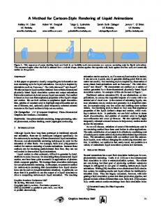
Figure 9: Velocity-dependent activation of examples leads to different wrinkles forming as the drape swings back and forth. Fig. 9 shows several frames from an animation of a swinging drape. The example activation is controlled as a function of the center of mass velocity, and as a result, different types of wrinkles form when the drape swings forwards and backwards. A similar strategy is used to control the deformations of the simulated plane shown in Fig. 10. As a function of the angle between the center of mass velocity and acceleration vectors we activate a potential that creates the impression that the plane is leaning into the turns. Figure 7: Our framework enables control over the wrinkles that form in simulated cloth. Left: no examples were used. Middle: The bottom part of the cloth appears to twist. Right: a very specific wrinkling pattern is prescribed.

Explicit Weight Control For the results discussed so far, naturally occurring deformations drive the activation of the input examples. However, as shown here, it can also be desirable to explicitly specify the activation patterns. For this purpose, Equation (3) can be easily modified to allow explicit control over the values of the weights associated with the input poses. As highlighted by McAdams et al. [MZS∗ 11], soft tissue simulation for character animation purposes has several benefits, including an automatic treatment of contacts and collisions. Our method adds another important ingredient to this line of research: artistic control over the deformation behavior of the simulation, as illustrated by the arm example (Fig. 8). Two artist-sculpted example poses, one where the arm is straight, and another where it is bent, were provided as input, and external forces were used to bend the arm. As a function of the joint angle of the elbow joint we increase the weight associated with the example pose, which is then treated as a hard constraint. The original artistic intent can be seen in the outcome of the simulation, as the muscles appear to flex in a natural way while exhibiting subtle dynamics. This application can be considered as a hybrid between trac 2012 The Author(s)

c 2012 The Eurographics Association and Blackwell Publishing Ltd.

Figure 10: A simulated plane appears to lean into the turns.

7. Limitations and Future Work We present an efficient way of simulating example-based, elasto-plastic shells and solids. At the core of our method is an incompatible shape representation which greatly simplifies interpolation on the manifold defined by a set of input shapes. As noted in [MTGG11], it is possible to provide input examples that counteract the deformations that an object naturally undergoes. As a result, those particular examples may not become active. While this remains a problem in general, the explicit weight control method that we experimented with could be used to give users additional control over the simulation results. Large deformations typically require a remeshing of the simulated objects. Our simulation environment requires the input examples to have the same topology as the object, and therefore they have to also be remeshed at the same

Schumacher et al. / Efficient Simulation of Example-Based Materials

Figure 8: The example activation is controlled by the joint angle of the arm, resulting in a flexed biceps as the arm bends.

time. This is an interesting direction for future work, as the remeshing operation needs to simultaneously ensure wellshaped elements for the deformed configuration as well as all the example poses.

References [ACOL00] A LEXA M., C OHEN -O R D., L EVIN D.: As-RigidAs-Possible Shape Interpolation. In Proc. of ACM SIGGRAPH ’00 (2000). 2 [BBO∗ 09] B ICKEL B., BÄCHER M., OTADUY M. A., M ATUSIK W., P FISTER H., G ROSS M.: Capture and modeling of nonlinear heterogeneous soft tissue. In Proc. of ACM SIGGRAPH ’09 (2009). 2 [BdSP09] BARBI Cˇ J., DA S ILVA M., P OPOVI C´ J.: Deformable object animation using reduced optimal control. In Proc. of ACM SIGGRAPH ’09 (2009). 2

[KMP07] K ILIAN M., M ITRA N. J., P OTTMANN H.: Geometric modeling in shape space. In Proc. of ACM SIGGRAPH ’07 (2007). 2 [LCF00] L EWIS J. P., C ORDNER M., F ONG N.: Pose space deformation: a unified approach to shape interpolation and skeleton-driven deformation. In Proc. of ACM SIGGRAPH ’00 (2000). 2, 7 [LSLCO05] L IPMAN Y., S ORKINE O., L EVIN D., C OHEN -O R D.: Linear rotation-invariant coordinates for meshes. In Proc. of ACM SIGGRAPH ’05 (2005), pp. 479–487. 2 [MTGG11] M ARTIN S., T HOMASZEWSKI B., G RINSPUN E., G ROSS M.: Example-based elastic materials. In Proc. of ACM SIGGRAPH ’11 (2011). 1, 2, 4, 6, 7 [MZS∗ 11] M C A DAMS A., Z HU Y., S ELLE A., E MPEY M., TAMSTORF R., T ERAN J., S IFAKIS E.: Efficient elasticity for character skinning with contact and collisions. In Proc. of ACM SIGGRAPH ’11 (2011). 7

[BMWG07] B ERGOU M., M ATHUR S., WARDETZKY M., G RINSPUN E.: TRACKS: Toward Directable Thin Shells. In Proc. of ACM SIGGRAPH ’07 (2007). 2, 5

[NMK∗ 06] N EALEN A., M ÜLLER M., K EISER R., B OXERMAN E., C ARLSON M.: Physically based deformable models in computer graphics. Computer Graphics Forum 25, 4 (2006), 809– 836. 2

[BP08] BARBI Cˇ J., P OPOVI C´ J.: Real-time control of physically based simulations using gentle forces. In Proc. of ACM SIGGRAPH Asia ’08 (2008). 2

[OBH02] O’B RIEN J. F., BARGTEIL A. W., H ODGINS J. K.: Graphical modeling and animation of ductile fracture. In Proc. of ACM SIGGRAPH ’02 (2002). 2

[BW97] B ONET J., W OOD R. D.: Nonlinear Continuum Mechanics for Finite Element Analysis. Cambridge Univ. Press, 1997. 5 [BWHT07] BARGTEIL A. W., W OJTAN C., H ODGINS J. K., T URK G.: A finite element method for animating large viscoplastic flow. In Proc. of ACM SIGGRAPH ’07 (2007). 2, 4 [CMT∗ 12]

C OROS S., M ARTIN S., T HOMASZEWSKI B., S CHU MACHER C., S UMNER R., G ROSS M.: Deformable objects alive! In Proc. of ACM SIGGRAPH ’12 (2012). 2

[FB11] F RÖHLICH S., B OTSCH M.: Example-driven deformations based on discrete shells. Comput. Graph. Forum 30, 8 (2011), 2246–2257. 2, 4 [GBB09] G ERSZEWSKI D., B HATTACHARYA H., BARGTEIL A. W.: A point-based method for animating elastoplastic solids. In Proc. of Symp. on Computer Animation (SCA) ’09 (2009). 2 [GHDS03] G RINSPUN E., H IRANI A. N., D ESBRUN M., S CHRÖDER P.: Discrete shells. In Proc. of Symp. on Computer Animation (SCA ’03) (2003). 4 [ITF04] I RVING G., T ERAN J., F EDKIW R.: Invertible finite elements for robust simulation of large deformation. In Proc. of Symp. on Computer Animation (SCA ’04) (2004). 2, 4 [KKA05] KONDO R., K ANAI T., A NJYO K.- I .: Directable animation of elastic objects. In Proc. of Symp. on Computer Animation (SCA ’05) (2005), pp. 127–134. 2

[STBG12] S KOURAS M., T HOMASZEWSKI B., B ICKEL B., G ROSS M.: Computational design of rubber balloons. In Proc. of Eurographics ’12 (2012). 2 [TPBF87] T ERZOPOULOS D., P LATT J., BARR A., F LEISCHER K.: Elastically deformable models. In Proc. of ACM SIGGRAPH ’87 (1987). 2 [TPS09] T HOMASZEWSKI B., PABST S., S TRASSSER W.: Continuum-based strain limiting. In Proc. of Eurographics ’09 (2009). 2 [WDAH10] W INKLER T., D RIESEBERG J., A LEXA M., H OR MANN K.: Multi-scale geometry interpolation. In Proc. of Eurographics ’10 (2010). 2 [WK88] W ITKIN A., K ASS M.: Spacetime constraints. In Proc. of ACM SIGGRAPH ’88 (1988). 2 [WMT06] W OJTAN C., M UCHA P. J., T URK G.: Keyframe control of complex particle systems using the adjoint method. In Proc. of Symp. on Computer Animation (SCA ’06) (2006). 2 [WRK∗ 10] W ICKE M., R ITCHIE D., K LINGNER B. M., B URKE S., S HEWCHUK J. R., O’B RIEN J. F.: Dynamic local remeshing for elastoplastic simulation. In Proc. of ACM SIGGRAPH ’10 (2010). 5 [WT08] W OJTAN C., T URK G.: Fast viscoelastic behavior with thin features. In Proc. of ACM SIGGRAPH ’08 (2008). 2

c 2012 The Author(s)

c 2012 The Eurographics Association and Blackwell Publishing Ltd.