Efficiently learning simple timed automata Sicco Verwer, Mathijs de Weerdt, and Cees Witteveen Delft University of Technology, P.O. Box 5031, 2600 GA, Delft, the Netherlands
[email protected]
Abstract. We describe an efficient algorithm for learning deterministic real-time automata (DRTA) from positive data. This data can be obtained from observations of the process to be modeled. The DRTA model we learn from such data can be used reason and gain knowledge about realtime systems such as network protocols, business processes, reactive systems, etc.
1
Introduction
We describe an efficient algorithm for learning a timed automaton model from observations. Timed automata (TAs) [1] are finite state models that model time explicitly, i.e. using numbers. They are insightful models that can be used to model and reason about real-time systems such as network protocols, business processes, reactive systems, etc. In practice, it can be very difficult to construct such an automaton by hand. That is why we are interested in automatically identifying these models from data. Data can be obtained from observations of the process to be modeled. This results in a set of time series of events: every time-step the events occurring in the system are measured and recorded. We assume that the process is stationary, i.e., time shift independent. Therefore, it does not matter exactly when these observations are initiated and stopped; The observed behavior remains the same. From this timed data, we could have opted to identify an untimed model that models time implicitly, i.e. using states instead of numbers. Examples of such models are the deterministic finite state automaton (DFA) and the hidden Markov model (HMM), see e.g., [7, 8]. The reason for modeling time explicitly is that modeling time implicitly results in an exponential blow-up of the model size: numbers use a binary representation of time while states use a unary representation of time. Thus, an efficient algorithm that learns a timed system using an untimed model is by definition an inefficient algorithm since it requires exponential time and space in the size of the timed model. In contrast, using the algorithms described in this paper, it is possible to learn simple types of timed models efficiently, i.e. in polynomial time. This paper is organized as follows. We first describe the exact model we want to learn (Section 2), called a real-time automaton [3]. Then, we give our algorithm for learning these models (Section 3). Our algorithm makes use of statistical tests in order to determine its actions. We explain how to calculate these tests and how our algorithm uses these tests (Section 4). We end with a discussion and conclusion regarding the algorithm and its uses (Section 5).
b
a b
a [6,∞)
a
b a [0,5] Fig. 1. A DRTA. The nodes of the graph are states, the arcs are transitions. Every transition has a label and a clock guard. When the clock guard is absent, it is always true, i.e., it is [0, ∞). The start state is indicated by an arc pointing to it from nowhere. For the purpose of this paper, it is not useful to indicate which states are final.
2
Real-time automata
We assume the reader to be familiar with the theory of languages and automata, see e.g., [8]. Our work focusses on learning algorithms for a simple timed automaton known as a deterministic real-time automaton (DRTA) [3]. Our learning algorithms are based on the state merging method for learning a DFA. The problem of learning DFAs has been the subject of many studies within the grammatical inference field, and the state merging method is currently the best method for solving it, see [2]. A DRTA is a timed language model. A timed language is a set of finite sequences of symbol-time value pairs τ = (s1 , t1 )(s2 , t2 ) . . . (sn , tn ) known as timed strings or time-stamped event sequences. Every time value ti ∈ N in such a timed string represents the time that has elapsed since the occurrence of the previous symbol (event). The structure of a DRTA is like that of a DFA. However, in addition to the DFA structure, every transition in a DRTA contains a boolean constraint, known as a clock guard. Such a clock guard is represented by an interval in N. We say that a clock guard G is satisfied by a time value t if t ∈ G. The clock guard G of a transition δ specifies at what time δ is allowed to be fired: δ can only be fired if the time t since the occurrence of the previous symbol satisfies G. In this way, the execution of a DRTA depends not only on the symbols, like a DFA, but also on the time between two consecutive symbols of a timed string. Figure 1 shows an example of a DRTA. An DRTA is formally defined as follows: Definition 1. A real-time automaton (RTA) is a tuple A = h Q, Σ, T, q0 , F i, where Q is a finite set of states, Σ is a finite set of symbols, ∆ is a finite set of transitions, q0 is the start state, and F ⊆ Q is a subset of final states. A transition δ ∈ ∆ in this automaton is a tuple hq, q0 , a, G i, where q, q0 ∈ Q are the source and target states, a ∈ Σ is a symbol known as the transition label, and G is a clock guard defined by an interval in N. An RTA is called deterministic (DRTA) if for every state q ∈ Q, every symbol a ∈ Σ, and every time value t ∈ N there exists exactly one transition hq, q0 , a, G i ∈ ∆ such that G is satisfied by t.
The transitions hq, q0 , a, G i of a DRTA A define the behavior of A as follows: whenever the automaton is in state q, reading symbol a, and the clock guard G is satisfied by the time since the previous symbol, then the automaton will move to state q0 . Extending this from smbol-time value pairs to timed strings leads to the definition of a run of a DRTA: Definition 2. A run of an DRTA h Q, Σ, ∆, q0 , F i over a timed string
( a1 , t1 ) . . . ( a n , t n )
is
a
finite
sequence
( q0 , 0)
t
1 −→
( q0 , t1 )
a
1 −→
a
t
n n (qn , tn ), such that for all 1 ≤ i ≤ n, (qn−1 , tn ) −→ (q1 , 0) . . . (qn−1 , 0) −→ there exists a hqi−1 , qi , ai , Gi i ∈ ∆, such that Gi is satisfied by ti . If the run of a DRTA is such that qn ∈ F, it is called an accepting run.
We call a pair (q, t) ∈ Q × N of a state and a time value a timed state. In a run a i +1
the subsequence (qi−1 , ti ) −→ (qi , 0) represents a state transition like in a DFA. t i +1
In addition to these, a DRTA makes time transitions represented by (qi , 0) −→ (qi , ti+1 ). A time transition of t time units can be viewed as moving from one timed state (q, v) to another timed state (q, v + t) while remaining in the same untimed state q. These time transitions effectively model the duration of events in the system or the amount of time spent in certain states of the system. A timed string ends in the last state of its run, i.e., it ends in qn . The set of all strings τ such that the run of A over τ is accepting is called the language L(A) of A. There exist many systems that can be modeled efficiently and intuitively using such a time dependent language. We learn such a language from examples by using an DRTA model and a modified state merging algorithm.
3
Identifying DRTAs
In previous work, we constructed an efficient algorithm for learning DRTAs from labeled data [9]. A high-level view of this algorithm is given in Algorithm 1. The algorithm receives as input a finite set S of example timed strings that are (assumed to be) generated by a timed system. The goal of the learning problem is to find a smallest DRTA model that is consistent with the input. The reason that this has to be a smallest model is the principle of Occam’s razor. This states that the simplest (smallest) explanation for some observations is the best explanation. As a bonus, smaller models are also easier to comprehend, and hence give more insight into the observed process. From the input set S, our algorithm constructs a prefix tree A. This prefix tree is a DRTA that is such that: – all the clock guards are equal to true (it disregards time values), – there exists exactly one path to any state (it is a tree), and – the run of A on any timed string from S ends in a state in A. Figure 2 shows an example of such a prefix tree. Starting from this prefix tree, our algorithm performs the most consistent merge or split as long as consistent merges or splits are possible.
Algorithm 1 State merging and splitting DRTAs Require: A set of timed strings S. Ensure: The result is a small consistent DRTA A. Construct a timed prefix A tree from S. while States can be merged or split consistently do Evaluate all possible merges and splits. Perform the most consistent merge or split. end while return The constructed DRTA A b
a
a
a b b
b
Fig. 2. A prefix tree for the input set {( a, 3)(b, 2), ( a, 4)(b, 2)( a, 4)( a, 5), ( a, 6)(b, 5)( a, 8), ( a, 9)(b, 4)(b, 2), (b, 4)(b, 2)}.
A merge (Figure 3) of two states q1 and q2 replaces q1 and q2 with a new state q3 . This new state q3 is the target and the source state of all transitions that have q1 or q2 as either their target or source state respectively. After this replacement, it is possible that A contains some non-deterministic transitions, i.e., there can be two transitions with q3 as their source state that have the same label and overlapping clock guards. These non-deterministic transitions are removed by the determinization procedure: continuously merging the target states of these transitions until none are left. This merge procedure is identical to a merge in the state merging algorithm for DFAs, see [2]. In [9], we introduced a transition splitting process in order to learn the clock guards of a DRTA. A split (Figure 4) of a transition δ, at time t replaces δ by two new transition δ1 and δ2 that that are identical to δ except for their clock guards. The clock guard of δ1 is such that it is satisfied by all clock values that satisfy δ up to time t, and the clock guard of δ2 is such that it is satisfied by all clock values that satisfy δ starting at time t. The timed strings from S that have a run over δ1 and δ2 are subsets of the timed strings from S that had an execution path over δ. Therefore, the prefix tree is recalculated starting from the new transitions δ1 and δ2 . We only allow a split of a transition if its target has not yet been merged. Splitting transitions can later (after some merges) result in two non-deterministic transitions that have partially overlapping clock guards. In this case, the determinize procedure first splits these transitions before merging their target states. This splitting continues until all non-deterministic transitions have identical clock guards. A merge of two states essentially learns the target state of a transition. A split of a transition learns the clock guard of a transition. The main loop of our algo-
a
b
a
a
M
b a
D
b
M b
b
a
D
a
b
b
b
Fig. 3. The merge operation. Left shows the original DRTA, right shows the result after merging the states labeled with M. In the right figure, D labels the first two states that are to be merged by the deteminization procedure.
Sa
b
a
a
a [0,5]
b b
b
b
a [6,∞] b
a
a
b b
a b
Fig. 4. The split operation. Left shows the original DRTA, right shows the result after splitting to transition to the transition labeled with S. The subtrees of the new transitions in the resulting DRTA are recalculated from the input set.
rithm continuously merges states and splits transitions until consistent merges or splits can no longer be performed. Because our algorithm learns either a clock guard or a target state of a transition in every iteration, our algorithm is capable of learning any DRTA. Furthermore, since a merge or a split will never be undone, and since there are only a polynomial amount of possible merges and splits, our algorithm requires time polynomial in the size of the input set S. There is one important part of Algorithm 1 that we left undefined: What does it mean to be consistent? In [9], the answer to this question was simple: The algorithm got a labeled data set as input and consistency was defined using these labels. However, for many applications this setting is unrealistic: Usually, only positive data is available. What to do in this case? Intuitively, a merge or split is consistent if the data from the input set agrees with the resulting DRTA. For example, suppose that our algorithm will be used to learn a DRTA model for an unknown process P that can be modeled using the DRTA of Figure 1. The data S obtained from P will be such the events observed at the beginning will be more or less similar to the evens observed after seeing ab. In our prefix tree, this implies that the start state can be merged consistently with the state reached by ab. Also, this data S will be that the events observed after seeing ( a, t), t ≤ 5, are more or less different from the events observed after seeing ( a, t0 ), t0 > 5. In our prefix tree, this implies that the start state will contain a transition with label a that can be split consistently with time value t = 5. Our consistency check is a check for similarity of events. A merge (split) is more consistent than another merge (split) if the observed events are more
(less) similar. Hence, in order to determine the most consistent merge or split, we require a measure for this similarity. The measure we use is based on the one used in an algorithm for learning DFAs using statistical tests [5]. In the next section, we show how additional statistics can be used to add the time information that is available in timed strings to this test.
4
Statistics for learning DRTAs
In this section, we show how to use statistics in order to determine how consistent a merge or split is. Basically, this test should test the null-hypothesis that the events that are observed after reaching a state q1 come from the same distribution as the events that are observed after reaching another state q2 . The algorithm for learning DFAs using statistics that our method is based on uses the Chi-square test to test this null-hypothesis [5]. However, the Chisquare test cannot be applied directly to sequences of events because their probabilities are dependent. Therefore, this test is used to only test whether the single events that are observed directly after reaching state q1 and q2 are differently distributed. The distributions of subsequent events are tested using separate Chi-square tests using the pairs of states that are merged by the determinization procedure. These separate tests are independent and every one of them results in a p-value. This is the probability (in the limit) that the observed distributions over single events, or something more extreme, occurs when the null-hypothesis holds. If this value is sufficiently low for any of these tests (less than 0.05), the null-hypothesis is rejected and the states cannot be merged consistently. This test is then applied to all pairs of mergeable states. If the nullhypothesis is not rejected for some pair of mergeable states, then the pair of mergeable states that resulted in the highest p-value are merged. We use similar procedure for testing the consistency of merges and splits in our algorithm. In addition to the Chi-square test, we used a KolmogorovSmirnov (KS) test in order to make use of the time values of timed strings. This test tests the null-hypothesis that the time values of occurrences of a particular event that are observed after reaching q1 and q2 are the same. Thus, for every pair of states, in addition to the single Chi-square test, |Σ| KS tests are performed (where |Σ| is the size of the alphabet). These KS tests are useful if the timing of certain events in the process depend on the state of the process. We believe this to be true for many real-time processes. Combining the Chi-square and KS tests results in many independent tests that are performed for determining the consistency of a single merge or split. Even if the events observed after reaching q1 and q2 come from the same (timed) distribution, the probability the one of these tests results in a sufficiently low p-value is high. Because of this, we use a method that combines all of these p-values into a single test, called Fisher’s method. Fisher’s method transforms the p-values from all the individual tests into values that should follow a Chisquare distribution. Whether this holds is then tested using a single Chi-square test. This results in a single p-value for the null-hypothesis for determining the
consistency of a single merge or split. We reject the null-hypothesis if this pvalue is less then 0.05. In our algorithm, the most consistent merge is the one that results in the highest p-value greater than 0.05. The most consistent split is the one that results in the lowest p-value less than 0.05. In the case that there are consistent merges and splits, our algorithm uses the following rules to determine which merge or split to perform: – Perform the most consistent split if its value is less than 0.01. – Otherwise, perform the most consistent merge if its value is greater than 0.1. – Otherwise, perform the most consistent split. The intuition behind these rules is that we prefer performing consistent splits to consistent merges, but not if this merge is much more consistent than the split. Using these tests and rules in our algorithm results in a state-merging and transition-splitting method for learning DRTAs from positive data.
5
Discussion and conclusions
We described an algorithm for learning deterministic real-time automata (DRTA) from positive data based on the state-merging method for learning a deterministic finite state automaton (DFA). The data consist of timed event sequences that are obtained by observing the process. Since the DRTA is a model for a stationary process, it does not matter exactly when these observations are initiated and stopped. From such data, the algorithm uses statistical tests in order to find a DRTA model that succinctly captures the behavior of this process. The resulting DRTA model is insightful and can be used to reason and gain knowledge about the observed process. The algorithm can be shown to be efficient, i.e., it requires time polynomial in the size of the observations. In the near future, we would like to report on the results achieved using our algorithm. We implemented and tested it on data generated from a randomly generated DRTA. The results are promising in that our algorithm finds DRTAs very similar to the original DRTAs. However, since our algorithm learns from only positive data, there is no negative data to test it against, and hence it is difficult to evaluate the performance of our algorithm. Even more difficult is the problem how to compare our method with other known methods that use a state-based representation of time, i.e., algorithms for learning deterministic finite state automata (DFAs) or hidden Markov models (HMMs). How to do this is an open problem that we intend to solve in future work. In the near future, we also plan to test our algorithm on real (non-generated) data. This data will be obtained from sensors that are installed on trucks. From their measurements we intend to learn models that describe different kinds of driving behavior.
In related work, there exists several algorithms that learn DFAs from positive data, for an overview see [2]. Actually, these algorithms learn a probabilistic DFAs (PDFA), i.e., a DFA with probabilities added to the transitions. The expressive power of these PDFAs is equivalent to that of HMMs [4]. Therefore, our algorithm essentially learns a probabilistic variant of DRTAs, which is likely equivalent to some timed variant of an HMM. It would also be interesting to compare our method to other timed variants of HMMs, such as hidden semi-markov models, see e.g., [6].
References 1. Rajeev Alur and David L. Dill. A theory of timed automata. Theoretical Computer Science, 126:183–235, 1994. 2. Colin de la Higuera. A bibliographical study of grammatical inference. Pattern Recognition, 38(9):1332–1348, 2005. 3. Catalin Dima. Real-time automata. Journal of Automata, Languages and Combinatorics, 6(1):2–23, 2001. 4. P. Dupont, F. Denis, and Y. Esposito. Links between probabilistic automata and hidden markov models: probability distributions, learning models and induction algorithms. Pattern Recognition, 2005. 5. Christopher Kermorvant and Pierre Dupont. Stochastic grammatical inference with multinomial tests. In ICGI ’02, pages 149–160. Springer-Verlag, 2002. 6. Kevin P. Murphy. Hidden semi-markov models (hsmms). unrefereed tutorial, 2002. 7. Lawrence R. Rabiner. A tutorial on hidden markov models and selected applications in speech recognition. In Proceedings of the IEEE, volume 77, 1989. 8. Michael Sipser. Introduction to the Theory of Computation. PWS Publishing, 1997. 9. Sicco Verwer, Mathijs de Weerdt, and Cees Witteveen. An algorithm for learning real-time automata. In Benelearn’07, pages 128–135, 2007.