recognize the cause-effect relationships between potential process ..... process faults and the quality variables can be represented as v. Îu y. +. = (3). Where. T p.
ENGINEERING DRIVEN CAUSE-EFFECT MODELING AND STATISTICAL ANALYSIS FOR MULTI-OPERATIONAL MACHINING PROCESS DIAGNOSIS Jian Liu, Jing Li, Jianjun Shi Department of Industrial and Operations Engineering University of Michigan Ann Arbor, MI 48105
KEYWORDS Root cause diagnosis, cause-effect relationship, predicted symptom vector, multistage manufacturing process. ABSTRACT Process fault identification for product quality improvement is a critical issue in both design and manufacturing, especially for multistage manufacturing processes. In this paper, an integrated approach is proposed to develop cause-effect models from engineering knowledge and to conduct associated statistical analysis of the measurement data. First, a cause-effect diagram and predicted symptom vectors (PSV) are formulated to recognize the cause-effect relationship between process variables and product qualities. Then factor analysis and factor rotating technique are employed to extract the relationships reflected from measurement data. Finally the potential process faults are identified by comparing predicted symptoms and extracted symptoms. A case study is conducted to demonstrate the effectiveness of the proposed methodology. 1. INTRODUCTION Variation reduction is essential to ensure the competence of manufacturers, which demands quick detection and identification of process changes and their underlying fault sources. Recent years witnessed the marked advance in
automated in-process sensing and data collecting technologies for measuring a large number of product/process features. The resulting volume of multivariate data creates tremendous potential for monitoring and diagnosing quality-related problems in the manufacturing process. Historically, Statistical process control (SPC) (Woodall and Montgomery, 1999) was adopted as a major technique to monitor quality and process. Recently, multivariate statistical tools, such as Principle Component analysis (PCA) (Jackson, 1980) were introduced in the quality control problems to extract the variation structure from measurement data. However, without interpretation with domain knowledge, the statistical methods provide little diagnostic capability. Researches have been launched to address the knowledge-based root cause diagnosis issues. Ceglarek, Shi and Wu (1994) firstly attempted to provide a reasoning mechanism based on the hierarchical model of the auto-body assembly process. State space modeling methodology is also developed to represent the geometrical relation between variation sources and the key product characteristics (Zhou, et. al., 2003). Although it successfully solves the diagnostic problem, the accompanied modeling efforts are tremendous. Li and Zuo (1999), following the Failure Modes and Effect Analysis (FMEA) procedure, proposed a hybrid approach to qualitatively diagnose the root cause of a semiconductors manufacturing process. The qualitative analysis of this approach significantly
simplifies its implementation. However, the conceptual representation of the process knowledge provides less potential for itself to be linked with measurement data. Above reviews identify the necessity of an approach to effectively integrate the engineering knowledge with existing statistical techniques. In this paper, a methodology is proposed to provide a platform for representing engineering knowledge in the format of cause-effect models. Multivariate statistical tools are employed to detect process changes and extract the variation patterns. The underlying process faults are identified through comparing statistical analysis results and the cause-effect relationships. The remainder of this article is organized as follows. Section 2 gives an overview of the methodology. Section 3 introduces the formulation of the knowledge representation and the procedure of generating the cause-effect diagram and predicted fault symptom descriptions. Statistical tools used for detecting process changes and extracting variation patterns are introduced in section 4, together with the detail of fault diagnose procedure. Section 5 provides a set of case studies to demonstrate the proposed methodology and section 6 lists conclusions and some discussion. 2. OVERVIEW OF THE METHODOLOGY Root cause diagnosis for manufacturing process is a procedure that consists of five major tasks. (i) The engineering knowledge is organized and appropriately represented. (ii) Data collected from in-process sensing are tested to detect process changes (iii) Statistical analysis is launched to extract the implicit data patterns. (iv)Through linking the extracted data patterns with the engineering knowledge, potential fault sources are identified. (v)The diagnosis results can be used for process control or system maintenance for taking corrective actions. Corresponding to these tasks, a diagnosis methodology is proposed in this research. It consists of three main parts: knowledge representation, data analysis and fault identification, as shown in figure 1. Process planning information provides the basis for the engineering knowledge representation. The cause-effect diagram is formulated to recognize the cause-effect relationships between potential process faults and quality variables.
Fault predicted symptoms are pseudoquantitative descriptions of these relationships. The purpose of the data analysis is to detect the errors, extract their patterns and represent them in an interpretable format. Multivariate statistical tools are employed to recognize the spatial nature of faults’ impacts and provide adequate interpretability. By combining the engineering knowledge representation and statistical analysis of the measurement data, the process faults can be identified. Knowledge Representation
Data Analysis Measurement data
Process Information Precedence relation
Data Pre-process
Process Process Plan Plans
Cause - effect diagram Machine/ cutting Tool View
Datawith with Data Data with specific specific specific format format format
Data from CMM
Feature View
Data statistics
Fixture View
Error pattern extraction
Fault detection Fault symptom prediction Fault
Fault - symptom prediction
En gi ne
er in g
Symptom
Fault symptom estimation
Effect description
Causes Descriptions
...
Faults Identification Kn ow led
Symptom mapping ge
Confidence Evaluation ...
ic i st at St
ys al An al
is
FIGURE 1. OVERVIEW OF THE METHODOLOGY
3. KNOWLEDGE REPRESENTATION Often times, the lack of detailed description of manufacturing processes would hinder effective troubleshooting when problems occur. In this section, new concepts are proposed for representing the engineering knowledge and interfacing with statistical analysis results. 3.1 Formulation of cause-effect diagram The first step of cause-effect modeling is to define the process flow and machine datum strategy selected for real process. Traditionally, precedence diagram is one of the most powerful techniques to address this planning issue (Liu and Yuan, 1996). However, it describes only the precedence constraints among in-process features, not the quality variables and their relationships with process variables. Huang, et. al. (2000) proposed a similar strategy, D-graph, for the purpose of process diagnosability assessment. Although it is a good representation of datum strategy, D-graph has its limitation. It
records the precedence relations between datums and in-process features, but not the cause-effect relations in terms of impacts of a datum fault on the specific quality variables. Furthermore, besides the datums, error may also be introduced by fixtures, cutting tools and/or machine tools selected in each operation. If we adopt the assumption that the parts entering the system are perfect, these device-induced errors become the main source of potential root causes. Based on the above analysis, the requirements for a knowledge representation include: (i) it should be able to describe the precedence information, (ii) potential process faults should be included as complete as possible, and (iii) the cause-effect relationships between process faults and affected quality variables should be expressed explicitly.
• •
•
• •
features (e.g. Dk:h, the hth datum features used in operation k). The directed connections, , between them represent the precedence constraints. Triangle nodes, , denote the cutting tools and machine tools (e.g. CTk:r, the rth cutting tool used in operation k) selected to perform the manufacturing tasks. The directed connections, , from triangle nodes to circle nodes specify that the pointed features are generated by the pointing cutting tool and/or the pointing machine tool. The square nodes, , denote the fixture (e.g. FXk:w, the wth fixture used in operation k) scheme selected to locate the work piece. The triangle nodes and square nodes are connected only to the in-process features in the same operation.
In this approach, all the quality variables of the in-process features are effect elements. For the causes, there are 3 types of faults considered. (i) Machine and cutting tool faults, which are defined as the deviation of the cutting tools from their nominal path. (ii) Fixture faults, which are defined as the imperfection of the locators. (iii) Datum faults, which are defined as nonconformance of the in-process features used as datums in later operation(s).
FIGURE 2. CAUSE-EFFECT DIAGRAM FORMULATION
Process FMEA is a group of activities intended to recognize and assess the potential failure modes associated with the manufacturing processes or quality concerns and to understand the effects of them (Prasad, 1991). Inspired by the FMEA technique and D-graph representation, this paper presents the cause-effect diagram, as shown in figure 2. Process planning provides the information of devices (e.g. machine tool, cutting tools, fixtures, etc.), the precedence relations, datum strategies and in-process features formed in each operation. Figure 2 (a) is a partial description of them, where the following notations are adopted: • The circle nodes, , denote the in-process features (e.g. F(k-s):q , the qth feature generated in operation k-s.) and datum
As shown in figure 2 (b), the cause-effect diagram contains three views: feature view, fixture view and machine/cutting tools view. The layers in each view represent the operation sequence. In feature view, in-process features (e.g. Fk:2) are decomposed and expressed in terms of quality variables, i.e. the position (X, Y, Z), orientation (N) and dimension (D). These quality variables are deployed in different layers according to the precedence relations, and the directed connections between them represent the cause-effect relationships. For instance the connection from the X of F(k-s):q to the X of Fk:2 means that the imperfection of X position of datum feature F(k-s):q will cause the error of X position of the generated feature Fk:2. In feature view, connections appear only between the quality variables of datums and that of the inprocess features (generated based on those datums). In fixture view and machine/cutting tools view, nodes are also decomposed and expressed in terms of attributes of fixture and
machine/cutting tools. For instance, a locating pin FXk:w is described with its location (e.g. y) and size (e.g. d). Connections between these attributes and the quality variables also represent cause-effect relations. In the cause-effect diagram, all the nodes that have outgoing connections are cause nodes and those having incoming connections are effect nodes.
the 0-order predicted cause-effect relation between the ikth potential fault in operation k and the jth quality variable.
3.2 Predicted symptom representation
By stacking up all the n 0φik , j ’s according to the
The cause-effect diagram cannot be directly matched with the statistical analysis results. However, it contains the information about causes, affected quality variables and effect patterns, which is called symptom in this paper. The description of the symptom of a potential fault source should include following aspects:
operational sequence, the 0-order PSV of the ikth fault in operation k can be expressed as k0 f i k =[ 0φ i k ,1 , 0φ i k , 2 ,..., 0 φ i k , n ]T Those non-zero
(i) What quality variables are affected by one possible fault source? (ii) How are the effects exerted on those affected quality variables? (iii) How do the effects of a specific fault source propagate? The concept of predicted symptom vector (PSV) is proposed to capture those aspects. For a manufacturing process consisting of M operations, it can be known from the cause-effect diagram that there are totally n quality variables. For each operation k (k = 1, 2, … , M), there are mk potential faults and the total number of potential process faults is p, where p = Σ kM=1mk . Assuming that errors are introduced only by the devices (fixtures, tools and machines), therefore only device faults are included in mk. For a process fault ik and quality variable j, the impact of ik on j is defined as θ ik , j . It is time consuming, if not impossible, to derive the exact value of θ ik , j ’s. However, it is often comparatively easy to determine θ ik , j ’s sign and the interrelationship between
θ ik , j
and
θ ik ,l
,
(i.e
θ ik , j < θ i k , l or θ ik , j > θ ik , l ). For instance, if the positive deviation, in the fixture/machine coordinate system, of a process variable ik causes the quality variable j deviate along the positive direction, in the part coordinate system (Zhou, et. al, 2003), then θ ik , j > 0 , and vice versa. Therefore, in this approach, θ ik , j ’s are only represented pseudo-quantitatively. Let
φik , j be
0
⎧ 1, ⎪
if θi k , j > 0 if θi k , j = 0 ⎪− 1, if θ ik , j < 0 ⎩
(1)
φik , j = ⎨ 0,
0
Where k = 1,2,..., M ; ik = 1,2,..., mk and j = 1,2,..., n
φik , j ’s indicate the affected quality variables and
0
the sign of non-zero
φik , j ’s reflect how the
0
effects are exerted (i.e. if a process variable changes in positive direction, how this change is reflected at the quality variables). Meanwhile, the interrelations between effects are also critical for identifying and differentiating the faults, especially for the case that different faults (nonorthogonal to each other) affecting the same set of quality variables present simultaneously. 1order PSV describes these interrelations. Let
φi
1
k,j
⎧1 ⎪ ⎪ ⎪ ⎪0 ⎪ =⎨ ⎪ ⎪− 1 ⎪ ⎪ ⎪∞ ⎩
if 0φi
k,j
≠ 0, 0φi
if 0φi
k ,t
k,j
k ,t
and φi
(2)
≠ 0, θ ik , j < θ ik ,l ,
k ,l
k ,t
k,j
= 0 (t = l + 1, l + 2,..., j − 1)
≠ 0, 0φi
0
if 0φi
≠ 0, θ ik , j = θ ik ,l ,
k ,l
and φi
k,j
= 0 (t = l + 1, l + 2,..., j − 1)
≠ 0, 0φi
0
if 0φi
≠ 0, θ ik , j > θ ik ,l ,
k ,l
and φi 0
= 0 (t = l + 1, l + 2,..., j − 1)
= 0 or
φi
0
k ,v
= 0 for all v < j
φik , j reflects the interrelation between magnitude
1
of the jth effect and that of the previous non-zero effect. So, 1-order PSV 1 1 1 1 T f = [ φ , φ ,..., φ ] . k ik i k ,1 ik , 2 ik , n For the error propagation consideration, since the in-process features generated in one stage may be selected as the datums, their imperfections will bring errors to the features generated based on them even when there is no process faults present in later operations. Due to their pseudo-quantitative nature, PSV’s are not capable to describe the propagated effects. However, a process fault affects only specific quality variables of the features generated in the same operation. For the quality variables of features generated in other operations, the
corresponding
φik , j ’s equal to 0 and 1φik , j ’s
0
equal to ∞ . Also because the statistical analysis tool introduced in section 4.2 has the capability to identify this difference, it is rational to dismiss from PSV’s the description of propagated effects. 4. STATISTICAL DATA ANALYSIS To implement the root cause diagnosis, PSV’s should be compared with the symptoms extracted from in-process measurements. In this paper, the linear cause-effect relationships between dimensional quality and process variables are adopted based on the assumption that process faults are often small in magnitudes. Thus, a general nonlinear relationship can be approximated through Taylor series expansion around its nominal value. Let y = [ y1 y2 K y n ]T be an n×1 random vector formed by stacking up quality variables of the in-process features generated in different operations. Those variables are defined as the deviation from nominal value. Let yi (i=1,2,…,N) be a random sample of N observations of y. The cause-effect relationship between potential process faults and the quality variables can be represented as y = Γu + v
Where u = [u1 u 2
(3) ... u p ]T is a p×1 random
vector that represents the p ( p ≤ n ) potential faults (i.e. causes). Γ = [ϕ1 ϕ 2 ... ϕ p ] is an n by p constant matrix determined by product design and process plan. ϕ j (j = 1, 2, … , n) is an
n×1 vector. v = [v1 v2 K vn ]T is an n×1 zeromean random vector with covariance matrix Σ v = σ 2 I n×n , where In × n denotes an n by n identity matrix. The process faults defined in u often manifest themselves as mean shifts and/or increase of variances. As a result, u is split into two parts: a deterministic part u and a zero-mean random ~ . So, Eq. (3) can be written as: part u ~ ) + v = Γ u + Γu ~+v y = Γ(u + u
(4)
Where u = Ε(u ) is a deterministic vector, ~ = u - u and v are independent zero-mean u
random vectors. When process faults present, the measurement data will correspondingly demonstrate shift of mean and/or increase of variance. Let y = y + ~ y, y = Γu ~ ~+v y = Γu
(5) (6)
The objectives of the statistical analysis include: (i) detecting the process changes from measurement data and (ii) extracting the spatial nature of the process faults, i.e. the fault directions ϕ k ’s, and (iii) matching them with PSV’s to identify the potential process faults. According to Eq. (5) and (6), the process faults manifest as mean shifts have fixed effects on quality variables and those manifest as variance increase cause random effects. In this paper, the identification of the fault sources which cause random effects is addressed. 4.1 Hypothesis testing for fault detection Assume that the measurement data y follows multivariate normal distribution. Suppose totally N random samples are measured and denoted by Y = [y1 y 2 ... y N ]T . From (3), under normal manufacturing condition, µY = 0 and Σ Y = diag (σ 12 , σ 22 , ... σ n2 ) , where µ Y and
Σ Y represent the mean vector and covariance matrix of respectively. Apley and Shi (2001) discussed the applicability to assume that the covariance matrix of Y is a diagonal matrix with equal diagonal elements, i.e. Σ Y = σ 2 I . Process fault will result in a different variation pattern. Hence, statistical hypotheses testing on sample covariance can be conducted to detect the process changes. H 0 : Σ Y = σ 2 I vs. H a : Σ Y ≠ σ 2 I
(7)
Where, σ 2 is an unknown positive value. The test is based on the unbiased likelihood ratio statistic
λ = S /( n −1tr (S)) n
(8)
Where, S = ( N − 1) −1 Σ iN=1 (y i − Y )( y i − Y )T . At the
α th level of significance, it rejects H 0 in favor of H a if the observed statistic − [( N − 1) − ( 2n 2 + n + 2) / 6n] log λ > χ g2 ,α
(9)
Where, χ g2,α distribution
is an asymptotical chi-square
g = n( n + 1) / 2 − 1 degrees
with
of
freedom. If H0 is rejected at significance level α , it means that process faults, which manifest themselves as variance increase, are present.
symptom vectors (ESV)”, which can be compared with the PSV’s to identify the faults. To and 1-order ( ϕ = [ ϕ 1
Σ Y = Cov( Y) = E( Y − µ Y )(Y − µ Y ) T = ΓΓ T + Ψ
(10)
have eigenvalue-eigenvector pairs ( λ i , e i ) with
λ1 ≥ λ2 ≥ K ≥ λ p ≥ 0 and span{e i }ip=1 = span{ϕ i }ip=1 , ~ ) = 0 and Cov( u ~ ) = I , Σ can and assume that E (u Y
be decomposed as: Σ Y = Z p Λ p Z p + diag {ψ 1 ,ψ 2 ,K ,ψ n }
(11)
Where Z p = [e1 , e2 ,Ke p ] , Λ p = diag {λ1 , λ2 ,K, λ p } ,
ψ i = σ ii − ∑ pj=1ϕ ij2
for i=1,2,…,n. Matrix Γ can be
∗ i
1
0 ∗
ϕ
i, j
1 ∗ ϕi , j
⎧ 1, ⎪⎪ = ⎨ 0, ⎪ − 1, ⎩⎪
ϕ
∗ i ,1
are formulated for each
4.2 Symptom extraction for fault identification
~ ) = 0 and Cov( u ~ ) = I , Eq. (6) can Assuming E (u be treated as an orthogonal factor model with p common factors (Richard and Dean, 1998). Therefore, factor analysis is used in this paper to identify the linear cause-effect relationship between quality variables and process faults. The p common factors are the process faults needed to be figured out. Under the assumption of linear relationship, the covariance between ~ measurement data Y and the random process ~ ~ ~ faults u is defined by Cov( Y , u ) = Γ . Principal component method is used to estimate the factor loading matrix Γ . Let the covariance of Y,
[
implement it, 0-order ( 0 ϕ∗i = 0ϕi∗,1 1
∗ i,2
ϕ i∗ ( i
0 ∗ ϕi , 2
K
ϕ
1
K
]
∗ T i ,n
])
0 ∗ T ϕi , n
) ESV’s
= 1,2,K , p ). Let
if ϕ i , j > 0 and ϕ i , j > h
(13)
if ϕ i , j < h if ϕ i , j < 0 and ϕ i , j > h
⎧1 if 0ϕi∗, j ≠ 0, 0ϕi∗,k ≠ 0, ϕi∗, j > ϕi∗,l , ⎪ and ϕi∗,t = 0 (t = l + 1, l + 2,..., j − 1) ⎪ ⎪0 if 0ϕi∗, j ≠ 0, 0ϕi∗,k ≠ 0, ϕi∗, j = ϕi∗,k , ⎪⎪ =⎨ and ϕi∗,t = 0 (t = l + 1, l + 2,..., j − 1) ⎪− 1 if 0ϕ ∗ ≠ 0, 0ϕ ∗ ≠ 0, ϕ ∗ < ϕ ∗ , i, j i ,k i, j i ,k ⎪ ⎪ and ϕi∗,t = 0 (t = l + 1, l + 2,..., j − 1) ⎪ 0 ∗ 0 ∗ ⎪⎩ ∞ if ϕi , j = 0 or ϕi ,v = 0 for all v < j
(14)
Where i = 1,2,..., m and j = 1,2,..., n and h is a positive threshold. As discussed in section 3, process faults that are present in different operations cause different effects. The factor analysis (Richard and Dean, 1998) and factor rotation techniques tend to find the loading structure that each factor (process fault) has high contribution to some variables and small contribution to the others. Therefore, factor analysis provides the capability to identify this difference and to distinguish process fault present in different operations. The extracted symptom vectors for each individual operation k0 ϕ ∗i and k1 ϕ ∗i ( k = 1,2, K , M ) ϕ∗i and 1 ϕ∗i , as illustrated in
estimated by Z p Λ −p1/ 2 . The number of process
are derived from
faults equals to the number of retained principle components p ( p ≤ n ). Let T be a p×p orthogonal
figure 3. Each k0 ϕ ∗i or k1 ϕ ∗i contains n (total number of quality variables) elements. The elements corresponding to manufacturing features generated in operation k are copied from 0 ϕ ∗i
matrix, so that TT T = T T T = I . Eq. (6) can be written as
α
~ ∗ = TT u ~ has the same statistical properties u ~ . The loading Γ ∗ = ΓT = Z Λ −1 / 2 T can be as u p p
ϕi∗ [0 0 K K 0 0 1 0 K K 1 0 K K K 0 1 K K 0 1]
α ∗ 1 i
ϕ
[0
0 K K0 0 0 0 K K 0 0 K K K 0 0 K K 0 0]
α ∗ 2 i
[0
0 K K0 0 1 0 K K 1 0 K K K 0 0 K K 0 0]
ϕ
α ∗ M i
{
distinguished from Γ . This is very much akin to clarifying the cause-effect relations between a specific process fault and the quality variables. So in this research, the rotated factor loadings ϕ ∗i ’s ( i = 1,2,K , p ) are “extracted
{
(12)
{ { { {
~ ~ + v = ΓTT T u ~ + v = Γ∗u ~∗ + v y = Γu
0
ϕ [0 0 K K 0 0 0 0 K K 0 0 K K K 0 1 K K 0 1]
FIGURE 3. DECOMPOSITION OF ESV
and 1 ϕ ∗i , respectively. Other elements, which represent the quality variables of manufacturing features generated in other operations, are set to zeros. As a result, every 0 ϕ ∗i (or 1 ϕ ∗i ) has M (or
1 ∗ k ϕi
index k ∗ of the k0 ϕ ∗i ’s that contain non-zero elements indicates the stage where the fault introduced. In Figure 3, k ∗ = 2 . And, k0∗ ϕ ∗i ’s and
1 ∗ ϕ k∗ i
respectively. Let k0κ i: jk and
1 k κ i: jk
be the 0-order
and 1-order matching vectors (MV), respectively, 0 k κ i: j k
= k 0∗ ϕ∗i − k0f jk
(15)
1 k κ i: j k
= k ∗1ϕ∗i − k1f jk
(16)
Also let 0-order = number of
0 k ρ i: jk
matching index (MI) non-zero elements in
/ n and 1-order MI
1 k ρ i: jk
= number of non-
zero elements in k1κ i: jk / n . These two indices evaluate the confidence of the matching conclusion. Therefore, fault identification is a procedure to find the j that maximize k0 ρ i: jk and 1 k ρ i: jk
1
11 21 31 41 51 61 71 81 91 101 111 121 131 141 151 161
’s with non-zero elements will be
compared with k0 f j k ’s and k1 f j k ’s (jk =1,2,…,mk),
0 k κ i: j k
Extracted Symptoms
), k = 1,2, K , M . The smallest Magnitudes
0 ∗ k ϕi
Their corresponding PSV’s are listed in table 1 and table 2. 1,000 samples were simulated with the SS model and the corresponding measurements were generated.
.
5. CASE STUDY A case study was conducted by applying the proposed methodology in a real engine head machining process. The detailed process description and state space (SS) model introduced by Zhou, et. al. (2003) were used in this paper to derive cause-effect diagram and PSV’s of potential faults, simulate process faults and generate corresponding measurement data. Totally 168 quality variables of 28 features generated in 3 different operations were considered in y. Two faults were purposely introduced to operation 3 by: (i) Adding a variance source (fault 1) to the process variable corresponding to the X position of the 4-way pin, and (ii) Adding a variance source (fault 2) to the process variable corresponding to the X position of the 2-way pin.
Quality variables
ϕ1∗ Fault Dir2 Extracted
ϕ∗2 Fault Dir1 Extracted
FIGURE 4. EXTRACTED SYMPTOMS
Hypotheses testing results indicated the process changes. For the purpose of root cause diagnosis, two ESV’s were achieved by applying the FA on the simulated measurement data. These two ESV’s, as shown in figure 4, were compared with all the PSV’s of potential faults. The detailed 0-order and 1-order comparisons between the two ESV’s and the PSV’s of the two faults are listed in table 1 and table 2, respectively. Resultant MI’s indicated that ESV 1 was identified as fault 2 and ESV 2 was identified as fault 1. 6. CONCLUSION In this paper, a methodology for detecting and identifying process faults of multi-operational manufacturing system is proposed. It avoids time-consuming quantitative modeling and provides an effective representation of the engineering knowledge. The limitations of the current works include: (i) Different statistical analysis tools are required to extract the different variation patterns. (ii) Sensitivity analysis is another critical issue to be addressed, especially for the cases that the fault directions of two or more potential faults are not orthogonal to each other. (iii) A systematic mechanism to assess that identification result, especially for the nonorthogonal faults identification, is desirable. These limitations define the scope and directions of the future work. ACKNOWLEDGEMENT The author gratefully acknowledges the financial support of the NSF/ERC for Reconfigurable Manufacturing Systems (NSF Grant EEC95-92125).
TABLE 1. 0-ORDER MATCHING FOR FAULT IDENTIFICATION
Identification of fault 1 0-order PSV
0-order ESV’s
Identification of fault 2
f = [01× 48 | 01× 48 | Ξ −1 Ξ −1 Ξ −1 Ξ1
0 3 1
0 3
f 2 = [01×48
| 01×48 | Ξ 1
Ξ −1 Ξ −1 Ξ −1 Ξ −1 Ξ −1 Ξ −1
Ξ −1
Ξ −1
Ξ −1 Ξ1 ]T 0 ∗ 0 ∗ ϕ 2 = 3 ϕ 2 = [01×48 | 01×48 | Ξ −1 Ξ −1 Ξ −1
Ξ −1
Ξ −1 ]T
Ξ1 Ξ −1 ∗ 2
Ξ −1 Ξ −1
Ξ −1 Ξ −1
Ξ −1
Ξ −1 Ξ −1 ]T 0 3
0 3
Ξ −1
Ξ −1 Ξ −1 Ξ −1 Ξ −1 Ξ1 Ξ −1
Ξ −1
Ξ 1 ]T
ρ 2:1 = 1
0-order MI
Ξ1
Ξ −1
ϕ1∗ = 30ϕ1∗ = [01×48 | 01×48 | Ξ1 Ξ −1 Ξ −1 Ξ −1
κ 2:1 = ϕ − f = 0168×1
0-order MV
0 3
Ξ −1
Ξ −1
0
0 3 1:2
0 3
Ξ −1
Ξ −1
∗ 2
κ = ϕ − 30f 2 = 0168×1
0 3 1
0 3
ρ1:2 = 1
TABLE 2. 1-ORDER MATCHING FOR FAULT IDENTIFICATION
1-order PSV
1-order ESV
1-order MV 1-order MI
Identification of fault 53 f = [∞1×48 | ∞1×48 | ∞1×6 Ω1 Ω1 Ω1
1 3 1
Identification of fault 43 1 3 f2
= [∞1×48 | ∞1× 48 | ∞1×6
Ω −1 Ω −1 Ω −1
Ω −1 Ω −1 Ω −1 Ω −1 Ω −1 Ω1
Ω1 Ω1 Ω1 Ω1 Ω1 Ω −1
Ω1 Ω1 ]T
Ω −1 Ω −1 ]T
ϕ 2∗ = [∞1× 48 | ∞1×48 | ∞1×6
1 3
Ω −1
Ω −1
Ω1
Ω1 ] T
Ω0
Ω −1
Ω1
Ω1
Ω −1
∗ 2
1 3 1
ϕ = [∞1×48 | ∞1×48 | ∞1×6
1 ∗ 3 1
Ω1
Ω1
κ = ϕ − f = [01×132 − 1 01×35 ] ρ = 167 / 168 = 0.994
1 1 3 2:1 3 1 3 2:1
Ω1
Ω −1
Ω1
Ω1
Ω1
Ω −1
Ω1
Ω −1
Ω −1
Ω −1
Ω −1 ]T
1 ∗ 3 1
κ = ϕ − 31f 2 = 0168×1 ρ =1
1 3 1:2 1 3 1:2
Where Ξt =[t 0 0 0 0 0], Ωt = [t ∞ ∞ ∞ ∞ ∞] , ∞1×n = [∞ ∞ ... ∞]1×n and 01×n = [0 0 ... 0]1×n REFERENCES Apley, D. and Shi, J., (2001), “A Factor-Analysis Method for Diagnosing Variability in Multivariate Manufacturing Processes”, Technometrics. Vol. 43, No.1 pp84 – 95 Ceglarek, D. and Shi, J., (1995), "Dimensional Variation Reduction for Automotive Body Assembly", J. of Mfg. Review, Vol. 8, pp139-154. Huang, Q., Zhou, N. and Shi, J., (2000), “Stream of Variation Modeling and Diagnosis of Multistation Machining Processes”, Proc. 2000 ASME IMECE, MED-Vol. 11, pp.81-88, November, Orlando, FL. Jackson, J. E. (1980), “Principal Components and Factor Analysis: part I – Principal Components,” J. of Quality Tech., Vol. 12, pp201-213 Li, H. X., Zuo, M. J., (1999), “A hybrid approach for identification of root causes and reliability improvement of a die bonding process- a case study”, Reliability Eng. & Sys. Safety, Vol. 64, pp43-48.
Liu, T. I. and Yuan, G., (1996), “PDES - an expert system for constructing the precedence diagram”, J. of the Franklin Inst., v 333B, n 6, p 975-990. Prasad, S., ( 1991), “Improving manufacturing reliability in IC package assembly using the FMEA technique”, IEEE Trans. on Components, Hybrids and Mfg. Tech., v 14, n 3, Sep, p 452456. Richard A. J., Dean W. W., (1998) “Applied Multivariate Statistical Analysis”, Prentice Hall. Woodall, W. H. and Montgomery, D. C., (1999), “Research Issues and Ideas in Statistical Process Control”, J. of Quality Tech., Vol.31, pp376-386. Zhou, S., Huang Q. and Shi J., (2003), “State Space Modeling of Dimensional Variation Propagation in Multistage Machining Process Using Differential Motion Vector”, IEEE Trans. on Robotics and Automation, Vol. 19, No. 2, pp296309.