Entity Resolution in the Web of Data

UNIVERSITY OF CRETE DEPARTMENT OF COMPUTER SCIENCE FACULTY OF SCIENCES AND ENGINEERING

Entity Resolution in the Web of Data

by

Vasilis Efthymiou

PhD Dissertation Presented in Partial Fulfillment of the Requirements for the Degree of

Doctor of Philosophy

Heraklion, September 2017

UNIVERSITY OF CRETE DEPARTMENT OF COMPUTER SCIENCE Entity Resolution in the Web of Data PhD Dissertation Presented by Vasilis Efthymiou in Partial Fulfillment of the Requirements for the Degree of Doctor of Philosophy APPROVED BY :

Author: Vasilis Efthymiou

Supervisor: Vassilis Christophides, Professor, University of Crete, Greece

Committee Member: Dimitris Plexousakis, Professor, University of Crete, Greece

Committee Member: Yannis Tzitzikas, Associate Professor, University of Crete, Greece

Committee Member: Yannis Velegrakis, Associate Professor, University of Trento, Italy

Committee Member: Manolis Koubarakis, Professor, National and Kapodistrian University of Athens, Greece

Committee Member: Fabian Suchanek, Professor, Télécom ParisTech University, France

Committee Member: Grigoris Antoniou, Professor, University of Huddersfield, UK

Department Chairman: Angelos Bilas, Professor, University of Crete, Greece

Heraklion, September 2017

Dedicated to my parents, Panagiotis and Magdalini, and my sister, Maria.

Acknowledgments There are not enough words to express my deepest gratitude and respect to my PhD advisor, Professor Vassilis Christophides. His passion for research, his insight, and ability to always have the big picture, but above all, his personality and ethics, have been a true inspiration to me. I feel extremely lucky and honored to have met and worked with him. I also thank the members of my advisory committee, Professor Dimitris Plexousakis, and Associate Professor Yannis Tzitzikas, for their valuable comments and suggestions all these years. I am also grateful to the other members of my examination committee, Associate Professor Yannis Velegrakis, Professor Manolis Koubarakis, Professor Fabian Suchanek, and Professor Grigoris Antoniou. Their constructive comments, showing their expertise in the field, helped me improve this thesis. Special thanks to Prof. Suchanek for providing any information that I have asked about the source code and datasets used in his research. This is the right way, if not the only way, for research to progress, but unfortunately his stance was the exception, rather than the rule. I would like to deeply thank Associate Professor Kostas Stefanidis, the third member of our research team, for his great guidance and support. I owe him a lot and I feel that he has helped me improve in many aspects during our collaboration. I would also like to express my sincere gratitude to all my co-authors for their help and support throughout our collaboration. This PhD would not be the same without their significant contribution. Especially, I would like to thank Professor Themis Palpanas for his valuable contribution in this PhD and in my career. I would also like to thank Dr. Oktie Hassanzadeh and Dr. Mariano Rodriguez-Muro from IBM Research for our great collaboration and for providing an ideal working environment during my internship. A special mention is worth to Professor Timos Sellis for hosting me at RMIT, Melbourne. Seeing how much people within and outside the academia respect him both as a person and as a researcher has been inspiring. Meeting him in person has justified this level of respect. I would like to acknowledge the support of the Institute of Computer Science of the Foundation of Research and Technology (ICS-FORTH), and especially the Information Systems Laboratory (ISL), for both the financial support and the facilities. In particular, I thank the Head of ISL, Professor Dimitris Plexousakis, as well as all the faculty and staff members of ISL, for creating a highly creative and inspiring environment for me. Furthermore, I would like to thankfully acknowledge the support of DIACHRON (EU FP7-ICT-2011-9), SemData (EU FP7-PEOPLE- 2013IRSES), and IdeaGarden (EU FP7-ICT-318552). Part of my dissertation was supported and influenced by these projects. During this PhD, I was fortunate to meet many exceptional and inspiring friends and col-

vii

leagues: Kostas Petrakis, Dimitra Zografistou, Argyro Avgoustaki, Katerina Papantoniou, Pavlos Fafalios, Yannis Marketakis, Chrysostomos Zeginis, Ioannis Chrysakis, Thanos Yannakis, Nikos Minadakis, Giannis Roussakis, Georgia Troullinou, Konstantina Konsolaki, Vassilis Papakonstantinou, Aleka Seliniotaki, Mingzhao (Kane) Lee, Lance Song, Farhana Choudhury, Xiaolu Lu, Josep Pon Farreny, Siddharth Jain, Varun Chandramouli, Sanjay Surendranath Girija, Bilge Acun, Bogdan Ghit, Nicolas Fauceglia, Victor Han, Ioannis Petromichelakis, Ioannis Liodakis, and Giorgos Lyronis. Special thanks to Panagiotis Papadakos and Vangelis Kritsotakis for their valuable help in setting up and using the ISL cluster for the last part of this PhD. Last but not least, I would like to thank Myrto for her patience, love and support during the last four years. This PhD is dedicated to my parents, Panagiotis and Magdalini, who have always stood by me and my sister in any possible way, teaching us that life is more about sharing than receiving, and to my sister, Maria, who has been a second mother for me and now a real mother of the most brilliant child I have ever met, my niece Marilia. I hope that one day I will become half as good a parent as they are.

Abstract Entity resolution (ER) is the problem of identifying descriptions of the same real-world entities among or within knowledge bases (KBs). In this PhD thesis, we study the problem of ER in the Web of data, in which entities are described using graph-structured RDF data, following the principles of the Linked Data paradigm. The two core ER problems are: (a) how can we effectively compute similarity of Web entities, and (b) how can we efficiently resolve sets of entities within or across KBs. Compared to deduplication of entities described by tabular data, the new challenges for these problems stem from the Variety (i.e., multiple entity types and cross-domain descriptions), the Volume (i.e., thousands of Web KBs with billions of facts, hosting millions of entity descriptions) and Veracity (i.e., various forms of inconsistencies and errors) of entity descriptions published in the Web of data. At the core of an ER task lies the process of deciding whether a given pair of descriptions refer to the same real-world entity i.e., if they match (problem a). The matching decision typically depends on the assessment of the similarity of two descriptions, based on their content or their neighborhood descriptions (i.e., of related entity types). This process is usually iterative, as matches found in one iteration help the decisions at the next iteration, via similarity propagation until no more matches are found. The number of iterations to converge clearly depends on the size and the complexity of the resolved entity collections. Moreover, pairwise entity matching is by nature quadratic to the number of entity descriptions, and thus prohibitive at the Web scale (problem b). In this respect, blocking aims to discard as many comparisons as possible without missing matches. It places entity descriptions into overlapping or disjoint blocks, leaving to the matching phase comparisons only between descriptions belonging to the same block. For this reason, overlapping blocking methods are accompanied by Meta-blocking filtering techniques, which aim to discard comparisons suggested by blocking that are either repeated (i.e., suggested by different blocks) or unnecessary (i.e., unlikely to result in matches) due to the noise in entity descriptions. To address ER at the Web-scale, we need to relax a number of assumptions underlying several methods and techniques proposed in the context of database, machine learning and semantic Web communities. Overall, the Big Data characteristics of entity descriptions in the Web of data call for novel ER frameworks supporting: (i ) near similarity (identify matches with low similarity in their content), (i i ) schema-free (do not rely on a given set of attributes used by all descriptions), (i i i ) no human in the loop (do not rely on domain-experts for training data, aligned relations, matching rules), (i v) non-iterative (avoiding data-convergence methods at several iteration steps), and (v) scalable to very large volumes of entity collections (massively parallel architecture needed).

ix

To satisfy the requirements of a Web-scale ER, we introduce the MinoanER framework. Our framework exploits new similarity metrics for assessing matching evidence based on both the content and the neighbors of entities, without requiring knowledge or alignment of the entity types. These metrics allow for a compact representation of similarity evidence that can be obtained from different blocking schemes on the names and values of the descriptions, but also on the values of their entity neighbors. This enables the identification of nearly similar matches even from the step of blocking. This composite blocking, accompanied by a novel composite Meta-blocking capturing the similarity evidence from the different types of blocks, set the ground for a non-iterative matching. The matching algorithm, built on a massively parallel architecture, is equipped with computationally cheap heuristics to detect matches in a fixed number of steps. The main contribution of MinoanER is that it achieves at least equivalent results over homogeneous KBs (stemming from common data sources, thus exhibiting strongly similar matches) and significantly better results over heterogeneous KBs (stemming from different sources, thus exhibiting many nearly similar matches) to state-of-the-art ER tools, without requiring any domain-specific knowledge, in a non-iterative and highly efficient way. Keywords:

Entity Resolution, Blocking, Meta-blocking, Linked Data, MinoanER Supervisor: Vassilis Christophides Professor Computer Science Department University of Crete

Περίληψη Η ανάλυση οντοτήτων είναι το πρόβλημα της αναγνώρισης περιγραφών των ίδιων οντοτήτων του πραγματικού κόσμου ανάμεσα σε διαφορετικές βάσεις γνώσης. Σε αυτή τη διδακτορική εργασία, μελετάμε το πρόβλημα την ανάλυσης οντοτήτων στον Παγκόσμιο Ιστό των ∆εδομένων, στον οποίο οι οντότητες περιγράφονται μέσω RDF γράφων, ακολουθώντας τις αρχές των ∆ιασυνδεδεμένων ∆εδομένων. Τα δύο κεντρικά προβλήματα της ανάλυσης οντοτήτων είναι: (α) πώς μπορούμε να υπολογίσουμε την ομοιότητα οντοτήτων αποτελεσματικά, και (β) πώς μπορούμε να αναλύσουμε σύνολα οντοτήτων εντός ή μεταξύ των βάσεων γνώσης αποδοτικά. Σε σχέση με την απαλοιφή διπλοτύπων περιγραφών οντοτήτων σε σχεσιακές βάσεις, οι νέες προκλήσεις για αυτά τα προβλήματα πηγάζουν από την Ποικιλία (πολλαπλοί τύποι οντοτήτων και διαϑεματικές περιγραφές), τον ´Ογκο (χιλιάδες βάσεις γνώσης στον Παγκόσμιο Ιστό με δισεκατομμύρια γεγονότα, που φιλοξενούν εκατομμύρια περιγραφές οντοτήτων), και την Εγκυρότητα (πολλές μορφές ασυνέπειας και λαθών) των περιγραφών οντοτήτων που δημοσιεύονται στον Παγκόσμιο Ιστό των ∆εδομένων. Στον πυρήνα της ανάλυσης οντοτήτων βρίσκεται η διαδικασία λήψης της απόφασης για το αν ένα δοθέν ζευγάρι περιγραφών αναφέρονται στην ίδια πραγματική οντότητα, δηλαδή αν ταιριάζουν (πρόβλημα α). Η απόφαση ταιριάσματος συνήθως εξαρτάται από την εκτίμηση της ομοιότητας δύο περιγραφών, με βάση το περιεχόμενο ή ακόμα και τις γειτονικές τους περιγραφές (για οντότητες διαφορετικών τύπων). Αυτή η διαδικασία είναι συνήθως επαναληπτική, καθώς οι αποφάσεις ταιριάσματος σε μία επανάληψη βοηθούν στη λήψη αποφάσεων σε επόμενες επαναλήψεις, χρησιμοποιώντας διάδοση ομοιότητας, έως ότου να μην βρίσκονται άλλες περιγραφές που ταιριάζουν. Το πλήθος των απαιτούμενων για τη σύγκλιση επαναλήψεων εξαρτάται από το μέγεθος και την πολυπλοκότητα των συλλογών περιγραφών οντοτήτων. Επιπλέον, το ταίριασμα ζευγαριών περιγραφών είναι εκ φύσεως τετραγωνικής πολυπλοκότητας ως προς το πλήθος των περιγραφών και άρα απαγορευτικό στην κλίμακα του Παγκόσμιου Ιστού (πρόβλημα β). Στο πλαίσιο αυτό, η συσταδοποίηση έχει στόχο να αποτρέψει όσο το δυνατόν περισσότερες συγκρίσεις, χωρίς να χαθούν ταιριαστές περιγραφές. Τοποθετεί τις περιγραφές οντοτήτων σε επικαλυπτόμενες ή μη-επικαλυπτόμενες συστάδες, προωθώντας στη φάση ταιριάσματος τις συγκρίσεις μόνο μεταξύ περιγραφών που έχουν τοποθετηθεί σε κάποια κοινή συστάδα. Οι μέθοδοι επικαλυπτόμενης συσταδοποίησης συνοδεύονται από τεχνικές Μετα-συσταδοποίησης, που έχουν ως στόχο την αποτροπή των επαναλαμβανόμενων ξι

συγκρίσεων που προτείνονται από πολλαπλές συστάδες, καθώς και των συγκρίσεων μεταξύ περιγραφών που είναι πιθανότερο να μην ταιριάζουν, αλλά έχουν προταθεί λόγω ύπαρξης ϑορύβου στις περιγραφές οντοτήτων. Για να αντιμετωπίσουμε το πρόβλημα της ανάλυσης οντοτήτων στην κλίμακα του Παγκόσμιου Ιστού, χρειάζεται να χαλαρώσουμε ένα πλήθος υποθέσεων που υπόκεινται πολλών μεθόδων και τεχνικών, οι οποίες έχουν προταθεί στις ερευνητικές κοινότητες των βάσεων δεδομένων, της μηχανικής μάθησης και του σημασιολογικού Ιστού. Συνολικά, τα χαρακτηριστικά Μεγάλων ∆εδομένων που εμφανίζουν οι περιγραφές οντοτήτων στον Παγκόσμιο Ιστό των ∆εδομένων απαιτούν νέα συστήματα ανάλυσης οντοτήτων που να υποστηρίζουν: (i) σχεδόν ομοιότητα περιγραφών (αναγνωρίζουν περιγραφές που ταιριάζουν και έχουν χαμηλή ομοιότητα περιεχομένου), (ii) ανεξαρτησία ύπαρξης σχήματος (δεν στηρίζονται στην ύπαρξη ενός συγκεκριμένου συνόλου γνωρισμάτων που χρησιμοποιούνται από όλες τις περιγραφές), (iii) πλήρη αυτοματοποίηση (δεν στηρίζονται σε ειδικούς της εκάστοτε περιοχής για δεδομένα εκμάθησης, αντιστοίχιση σχέσεων, κανόνες ταιριάσματος), (iv) μη-επαναληπτικότητα (οι επαναληπτικές μέθοδοι συγκλίνουν μετά από υπερβολικά πολλές επαναλήψεις στον Παγκόσμιο Ιστό των ∆εδομένων), και (v) κλιμακωσιμότητα σε πολύ μεγάλους όγκους δεδομένων (απαιτούνται μαζικά παραλληλοποιήσιμες αρχιτεκτονικές). Για να ικανοποιήσουμε τις απαιτήσεις ανάλυσης οντοτήτων στην κλίμακα του Παγκόσμιου Ιστού, εισάγουμε το σύστημα MinoanER. Το σύστημά μας εκμεταλλεύεται νέες μετρικές ομοιότητας για την εκτίμηση των ενδείξεων ταιριάσματος τόσο από το περιεχόμενο όσο και από τις γειτονιές των περιγραφών, χωρίς να απαιτεί πρότερη γνώση ή αντιστοίχιση των τύπων των οντοτήτων. Αυτές οι μετρικές επιτρέπουν μια συμπαγή αναπαράσταση των ενδείξεων ομοιότητας που μπορούν να αποκτηϑούν από διαφορετικά σχέδια συσταδοποίησης πάνω στα ονόματα και τις τιμές των περιγραφών, καθώς επίσης και στις τιμές των γειτονικών τους περιγραφών. Αυτό επιτρέπει την αναγνώριση σχεδόν όμοιων περιγραφών που ταιριάζουν νωρίς, από το βήμα της συσταδοποίησης. Η σύνθετη αυτή συσταδοποίηση, ακολουθούμενη από μία νέα σύνθετη Μετα-συσταδοποίηση που αποτυπώνει τις ενδείξεις ομοιότητα από διαφορετικού τύπου συστάδες, ϑέτουν τις βάσεις για ένα μη-επαναληπτικό ταίριασμα. Ο αλγόριθμος ταιριάσματος, σχεδιασμένος με μία μαζικά παράλληλη αρχιτεκτονική, χρησιμοποιεί υπολογιστικά φτηνές ευριστικές μεθόδους για να αναγνωρίσει περιγραφές που ταιριάζουν σε ένα προκαθορισμένο πλήθος βημάτων. Η κύρια συνεισφορά του MinoanER είναι ότι πετυχαίνει τουλάχιστον ισάξια αποτελέσματα σε ομοιογενείς βάσεις γνώσης (που έχουν κοινές πηγές και συνεπώς περιέχουν πολύ όμοιες περιγραφές οντοτήτων), και σημαντικά καλύτερα αποτελέσματα σε ανομοιογενείς βάσεις γνώσης (που έχουν διαφορετικές πηγές και συνεπώς περιέχουν λιγότερο όμοιες περιγραφές), σε σχέση με συστήματα αιχμής στην ανάλυση οντοτήτων, χωρίς να απαιτεί οποιαδήποτε γνώση ενός συγκεκριμένου πεδίου, με μη-επαναληπτικό και εξαιρετικά

αποδοτικό τρόπο. Λέξεις κλειδιά: Ανάλυση Οντοτήτων, Συσταδοποίηση, Μετα-συσταδοποίηση, ∆ιασυνδεδεμένα ∆εδομένα, MinoanER Επόπτης: Βασίλης Χριστοφίδης Καθηγητής Τμήμα Επιστήμης Υπολογιστών Πανεπιστήμιο Κρήτης

Contents Acknowledgments . . . . . . . . . . . . . . . . . . . . . . . . . . . . . . . . . . . . . . . . . . . .

vii

Abstract . . . . . . . . . . . . . . . . . . . . . . . . . . . . . . . . . . . . . . . . . . . . . . . . . .

ix

Περίληψη (Abstract in Greek) . . . . . . . . . . . . . . . . . . . . . . . . . . . . . . . . . . . . .

xi

Table of Contents . . . . . . . . . . . . . . . . . . . . . . . . . . . . . . . . . . . . . . . . . . . . .

xv

List of Figures . . . . . . . . . . . . . . . . . . . . . . . . . . . . . . . . . . . . . . . . . . . . . . . xvii List of Tables . . . . . . . . . . . . . . . . . . . . . . . . . . . . . . . . . . . . . . . . . . . . . . .

xix

1 Introduction . . . . . . . . . . . . . . . . . . . . . . . . . . . . . . . . . . . . . . . . . . . . . .

1

1.1 The Value of Entity Resolution . . . . . . . . . . . . . . . . . . . . . . . . . . . . . . . .

2

1.2 Entity Resolution Workflow . . . . . . . . . . . . . . . . . . . . . . . . . . . . . . . . . .

5

1.3 Requirements for a Web-scale Entity Resolution . . . . . . . . . . . . . . . . . . . . . .

7

1.4 Contributions and Outline . . . . . . . . . . . . . . . . . . . . . . . . . . . . . . . . . . .

10

2 Blocking . . . . . . . . . . . . . . . . . . . . . . . . . . . . . . . . . . . . . . . . . . . . . . . .

13

2.1 Introduction . . . . . . . . . . . . . . . . . . . . . . . . . . . . . . . . . . . . . . . . . . .

13

2.2 Formal Blocking Model . . . . . . . . . . . . . . . . . . . . . . . . . . . . . . . . . . . .

14

2.3 Related Work . . . . . . . . . . . . . . . . . . . . . . . . . . . . . . . . . . . . . . . . . . .

18

2.3.1 Schema-based Blocking . . . . . . . . . . . . . . . . . . . . . . . . . . . . . . . .

18

2.3.2 Schema-free Blocking . . . . . . . . . . . . . . . . . . . . . . . . . . . . . . . . .

20

2.4 Scaling Blocking Methods to Very Large Entity Collections . . . . . . . . . . . . . . . .

25

2.4.1 Token Blocking . . . . . . . . . . . . . . . . . . . . . . . . . . . . . . . . . . . . .

25

2.4.2 Attribute Clustering Blocking . . . . . . . . . . . . . . . . . . . . . . . . . . . . .

25

2.4.3 Prefix-Infix(-Suffix) Blocking . . . . . . . . . . . . . . . . . . . . . . . . . . . . .

27

2.5 Benchmarking Content-based Blocking Methods in the Web of Data . . . . . . . . . .

28

2.5.1 Datasets . . . . . . . . . . . . . . . . . . . . . . . . . . . . . . . . . . . . . . . . .

29

2.5.2 Quality Results . . . . . . . . . . . . . . . . . . . . . . . . . . . . . . . . . . . . .

31

2.5.3 Performance Results . . . . . . . . . . . . . . . . . . . . . . . . . . . . . . . . . .

38

2.5.4 Lessons Learned . . . . . . . . . . . . . . . . . . . . . . . . . . . . . . . . . . . .

38

2.6 Conclusion . . . . . . . . . . . . . . . . . . . . . . . . . . . . . . . . . . . . . . . . . . . .

39

3 Meta-Blocking . . . . . . . . . . . . . . . . . . . . . . . . . . . . . . . . . . . . . . . . . . . . .

41

3.1 Introduction . . . . . . . . . . . . . . . . . . . . . . . . . . . . . . . . . . . . . . . . . . .

41

3.2 Formal Meta-blocking Model . . . . . . . . . . . . . . . . . . . . . . . . . . . . . . . . .

44

3.3 Related Work . . . . . . . . . . . . . . . . . . . . . . . . . . . . . . . . . . . . . . . . . . .

48

3.4 Scaling Meta-Blocking to Very Large Entity Collections . . . . . . . . . . . . . . . . . .

50

3.4.1 Approach Overview . . . . . . . . . . . . . . . . . . . . . . . . . . . . . . . . . . .

50

xv

3.4.2 Stage 1: Block Filtering . . . . . . . . . . . . . . . . . . . . . . . . . . . . . . . . .

51

3.4.3 Stage 2: Preprocessing . . . . . . . . . . . . . . . . . . . . . . . . . . . . . . . . .

52

3.4.4 Stage 3: Pruning (WNP) . . . . . . . . . . . . . . . . . . . . . . . . . . . . . . . .

57

3.5 Load Balancing . . . . . . . . . . . . . . . . . . . . . . . . . . . . . . . . . . . . . . . . .

60

3.5.1 Default Load Balancing . . . . . . . . . . . . . . . . . . . . . . . . . . . . . . . .

61

3.5.2 MaxBlock Load Balancing . . . . . . . . . . . . . . . . . . . . . . . . . . . . . . .

61

3.6 Experiments . . . . . . . . . . . . . . . . . . . . . . . . . . . . . . . . . . . . . . . . . . .

64

3.6.1 Setup . . . . . . . . . . . . . . . . . . . . . . . . . . . . . . . . . . . . . . . . . . .

65

3.6.2 Load Balancing . . . . . . . . . . . . . . . . . . . . . . . . . . . . . . . . . . . . .

66

3.6.3 Time Efficiency . . . . . . . . . . . . . . . . . . . . . . . . . . . . . . . . . . . . .

70

3.6.4 Scalability . . . . . . . . . . . . . . . . . . . . . . . . . . . . . . . . . . . . . . . .

74

3.6.5 Qualitative Results . . . . . . . . . . . . . . . . . . . . . . . . . . . . . . . . . . .

75

3.6.6 Discussion . . . . . . . . . . . . . . . . . . . . . . . . . . . . . . . . . . . . . . . .

76

3.7 Conclusion . . . . . . . . . . . . . . . . . . . . . . . . . . . . . . . . . . . . . . . . . . . .

77

4 Entity Matching . . . . . . . . . . . . . . . . . . . . . . . . . . . . . . . . . . . . . . . . . . . .

79

4.1 Introduction . . . . . . . . . . . . . . . . . . . . . . . . . . . . . . . . . . . . . . . . . . .

79

4.2 Related Work . . . . . . . . . . . . . . . . . . . . . . . . . . . . . . . . . . . . . . . . . . .

81

4.3 Basic Definitions . . . . . . . . . . . . . . . . . . . . . . . . . . . . . . . . . . . . . . . .

83

4.3.1 Entity similarity based on values . . . . . . . . . . . . . . . . . . . . . . . . . . .

84

4.3.2 Entity similarity based on neighbors . . . . . . . . . . . . . . . . . . . . . . . . .

86

4.4 Blocking . . . . . . . . . . . . . . . . . . . . . . . . . . . . . . . . . . . . . . . . . . . . .

88

4.4.1 Composite Blocking Scheme . . . . . . . . . . . . . . . . . . . . . . . . . . . . .

88

4.4.2 Disjunctive Blocking Graph . . . . . . . . . . . . . . . . . . . . . . . . . . . . . .

88

4.4.3 Graph Weighting and Pruning Algorithms . . . . . . . . . . . . . . . . . . . . .

89

4.5 Non-Iterative Matching . . . . . . . . . . . . . . . . . . . . . . . . . . . . . . . . . . . .

91

4.5.1 Implementation in Spark . . . . . . . . . . . . . . . . . . . . . . . . . . . . . . .

94

4.6 Experimental Evaluation . . . . . . . . . . . . . . . . . . . . . . . . . . . . . . . . . . . .

94

4.6.1 Effectiveness Evaluation . . . . . . . . . . . . . . . . . . . . . . . . . . . . . . . .

98

4.6.2 Efficiency Evaluation . . . . . . . . . . . . . . . . . . . . . . . . . . . . . . . . . . 101 4.7 Conclusion . . . . . . . . . . . . . . . . . . . . . . . . . . . . . . . . . . . . . . . . . . . . 102 5 Conclusion and Future Work . . . . . . . . . . . . . . . . . . . . . . . . . . . . . . . . . . . . 105 5.1 Synopsis of Contributions . . . . . . . . . . . . . . . . . . . . . . . . . . . . . . . . . . . 105 5.2 Short-term Improvements . . . . . . . . . . . . . . . . . . . . . . . . . . . . . . . . . . . 106 5.3 Directions for Future Research . . . . . . . . . . . . . . . . . . . . . . . . . . . . . . . . 107 Bibliography . . . . . . . . . . . . . . . . . . . . . . . . . . . . . . . . . . . . . . . . . . . . . . . . 111 Glossary . . . . . . . . . . . . . . . . . . . . . . . . . . . . . . . . . . . . . . . . . . . . . . . . . . 119

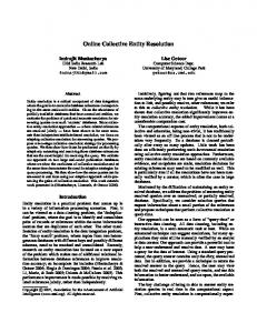
List of Figures 1.1 A part of the Web of data from two KBs: DBpedia (blue) and Freebase (red). Each table corresponds to an entity description, each header row to the URI of the described entity, and each other row to an attribute (left)- value (right) pair. . . . . . . . . . . .

3

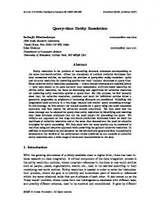
1.2 Searching for the entity “Stanley Kubrick” in the Web of data. . . . . . . . . . . . . . .

4

1.3 Outline of the entity resolution process. . . . . . . . . . . . . . . . . . . . . . . . . . . .

6

1.4 Value and neighbor similarity distribution of matching entities in 4 real dataset. . . .

8

2.1 A set of entity description. . . . . . . . . . . . . . . . . . . . . . . . . . . . . . . . . . . .

21

2.2 Token blocking example. Descriptions having a common token are placed in a common block. . . . . . . . . . . . . . . . . . . . . . . . . . . . . . . . . . . . . . . . . . . . .

21

2.3 Attribute clustering blocking example. Pairs of most similar attributes are linked (a). Connected attributes form clusters (b). Descriptions with a common token in the values of attributes of the same cluster, are placed in a common block (c). . . . . . .

22

2.4 Prefix-infix(-suffix) blocking example. A set of descriptions (a), their subject URIs (b), and the blocks from their tokens and infixes (c). . . . . . . . . . . . . . . . . . . . . . .

23

2.5 Token blocking in MapReduce. . . . . . . . . . . . . . . . . . . . . . . . . . . . . . . . .

26

2.6 Attribute clustering blocking in MapReduce. . . . . . . . . . . . . . . . . . . . . . . . .

26

2.7 Prefix-infix(-suffix) blocking in MapReduce. . . . . . . . . . . . . . . . . . . . . . . . .

27

2.8 Common tokens (top) and common tokens in common clusters (bottom) per entity description distributions for D1-D7. . . . . . . . . . . . . . . . . . . . . . . . . . . . . .

33

3.1 (a) A set of heterogeneous entity description, (b) the overlap-positive block collection derived from them using token blocking, (c) the respective blocking graph that uses Jaccard similarity for edge weights, (d) one of the possible pruned blocking graphs, and (e) the restructured block collection after Meta-blocking. . . . . . . . . .

42

3.2 (a) The serialized workflow of Meta-blocking, and (b) its parallelized counterpart. . .

50

3.3 Pseudo-code interpretation of (a) the basic and (b) the advanced strategy for Block Filtering. They employ a global and a local ordering of blocks, respectively. . . . . . .

51

3.4 An example of the advanced strategy for Block Filtering. . . . . . . . . . . . . . . . . .

53

3.5 Pseudo-code interpretation of the edge-based Preprocessing strategy, which explicitly creates the blocking graph. . . . . . . . . . . . . . . . . . . . . . . . . . . . . . . . .

54

3.6 Pseudo-code interpretation of the edge-based Preprocessing strategy for the EJS weighting scheme. . . . . . . . . . . . . . . . . . . . . . . . . . . . . . . . . . . . . . . .

xvii

55

3.7 Pseudo-code interpretation of the comparison-based Preprocessing strategy, which creates the blocking graph implicitly, enriching the description of the input block with the necessary information for weight estimation. . . . . . . . . . . . . . . . . . .

56

3.8 An example of the comparison-based strategy for Preprocessing. . . . . . . . . . . . .

56

3.9 Pseudo-code interpretation of the entity-based strategy for Preprocessing, which does not use the blocking graph. . . . . . . . . . . . . . . . . . . . . . . . . . . . . . . .

57

3.10 Pseudo-code interpretation of (a) the edge-based and (b) the comparison-based strategy for WNP. They share the same reduce function. . . . . . . . . . . . . . . . . . . .

58

3.11 An example of the comparison-based strategy for WNP, using the JS weighting scheme. . . . . . . . . . . . . . . . . . . . . . . . . . . . . . . . . . . . . . . . . . . . . . .

59

3.12 Pseudo-code interpretation of the entity-based strategy for WNP. . . . . . . . . . . .

60

3.13 An example of running MaxBlock for load balancing. . . . . . . . . . . . . . . . . . . .

63

3.14 Overhead Time in minutes for all configurations of the serialized workflow over DBC . 73 3.15 Speedup over DBC of (a) the comparison-based strategy for WEP, and (b) the entitybased strategy for CNP. . . . . . . . . . . . . . . . . . . . . . . . . . . . . . . . . . . . .

74

3.16 Average performance of the four pruning algorithms with respect to (a) Recall, (b) RR, (c) Precision, and (d) H 3R. . . . . . . . . . . . . . . . . . . . . . . . . . . . . . . . .

75

4.1 (a) Parts of entity graphs, representing the Wikidata (left) and DBpedia (right) KBs, (b) parts of the corresponding disjunctive blocking graph, and (c) the corresponding graph after pruning. . . . . . . . . . . . . . . . . . . . . . . . . . . . . . . . . . . . . . .

80

4.2 An example of running our heuristics on a pruned disjunctive blocking graph. . . . .

95

4.3 The architecture of MinoanER in Spark. . . . . . . . . . . . . . . . . . . . . . . . . . . .

96

4.4 Scalability of matching in MinoanER w.r.t. running time (left vertical axis) and speedup (right vertical axis) as more cores are involved. . . . . . . . . . . . . . . . . . . . . . . . 102 4.5 The area of matches from Figure 1.4 targeted by each of the employed heuristics. . . 103

List of Tables 2.1 Quality Measures. . . . . . . . . . . . . . . . . . . . . . . . . . . . . . . . . . . . . . . . .

17

2.2 Co-occurrence functions for considering two descriptions candidate match. . . . . .

24

2.3 Blocking methods with respect to the redundancy attitude and algorithmic attitude.

24

2.4 KBs characteristics. . . . . . . . . . . . . . . . . . . . . . . . . . . . . . . . . . . . . . . .

29

2.5 Datasets characteristics. . . . . . . . . . . . . . . . . . . . . . . . . . . . . . . . . . . . .

31

2.6 Statistics and evaluation of blocking methods. . . . . . . . . . . . . . . . . . . . . . . .

32

2.7 Characteristics of the missed match of token blocking. . . . . . . . . . . . . . . . . . .

36

2.8 Analysis of 1K sampled match and 1K sampled non-match. . . . . . . . . . . . . . . .

37

3.1 Summary of the notation used in Meta-blocking. . . . . . . . . . . . . . . . . . . . . .

45

3.2 The datasets employed in our experiments. . . . . . . . . . . . . . . . . . . . . . . . .

65

3.3 The block collections that were given as input to Meta-blocking. . . . . . . . . . . . .

66

3.4 The distribution of partition cardinalities produced by the default load balancer of Hadoop, PairRange and MaxBlock. . . . . . . . . . . . . . . . . . . . . . . . . . . . . . .

67

3.5 The wall-clock time (in minutes) of Meta-blocking using the default Hadoop balancer, the two variations of PairRange, and MaxBlock for the entity-based strategy over DBC , using the CBS weighting scheme across all pruning algorithms. The overhead of executing each load balancing algorithm, compared to the default balancing, is common for all pruning algorithms and is included in the wall-clock times. . . . .

69

3.6 The block collections after Block Filtering. . . . . . . . . . . . . . . . . . . . . . . . . .

70

3.7 Overhead Time (OT i me) in minutes for all Meta-blocking techniques across the four real datasets. . . . . . . . . . . . . . . . . . . . . . . . . . . . . . . . . . . . . . . . . . . .

71

4.1 KB statistics. . . . . . . . . . . . . . . . . . . . . . . . . . . . . . . . . . . . . . . . . . . .

97

4.2 Block statistics. . . . . . . . . . . . . . . . . . . . . . . . . . . . . . . . . . . . . . . . . .

98

4.3 Evaluation of MinoanER compared to existing methods. . . . . . . . . . . . . . . . . .

98

4.4 Evaluation of heuristics. . . . . . . . . . . . . . . . . . . . . . . . . . . . . . . . . . . . . 101

xix

Chapter 1

Introduction An increasing number of government organizations, local bodies, private companies, scientific or citizen communities are currently describing a great variety of real-world entities (e.g., persons, places, products, events) as Linked Data1 , in the form of RDF triples2 , i.e., subject-predicateobject facts. The emerging Web of data aims to support a global data infrastructure, in which realworld entities are described on the Web by data rather than documents. Exhibiting a higher degree of interoperability than documents and ease of reuse both by humans and machines, Linked Data emerges as a prominent paradigm for publishing structured information worldwide. Comprehensive, machine-readable entity descriptions are hosted in Knowledge Bases (KBs). Traditionally, KBs are manually crafted by a dedicated team of knowledge engineers (e.g., Wordnet3 and Cyc4 ); with the explosion of the Web, however, more and more KBs are built from existing Web content using information extraction tools [25]. Such an automated approach offers an unprecedented opportunity to scale-up KB construction and leverage existing knowledge published in HTML documents [50], but it also comes at the cost of a significant degree of redundancy in the descriptions provided across domains for the same real-world entities. Such KBs may contain complementary and sometimes conflicting information regarding the same entity, which could be combined in order to provide a more complete picture of the described entities than each individual KB offers and be exploited by a multitude of applications. A prerequisite for merging complementary information or repairing contradicting information is to identify first the descriptions that refer to the same real-world entity (called matches). This is the problem of entity resolution (ER), on which we focus in this work. This clearly requires an understanding of the similarity among described entities that goes beyond strong similarity studied in traditional deduplication and cleaning problems [76]. We essentially need to explore entity descriptions that are nearly similar [88], since those descriptions have been created by various extraction tools of different quality, focusing on different aspects of the entities.

1 http://linkeddata.org/ 2 http://www.w3.org/RDF 3 http://wordnet.princeton.edu 4 http://www.cyc.com

1

2

Chapter 1. Introduction

Example 1.1. Consider the entity descriptions presented in Figure 1.1. An entity description in the Web of data is an identifiable set of attribute-value pairs. In this example, the entity identifiers are given in the header rows and the attribute-value pairs are the remaining rows (attributes left, values right). The example shows entity descriptions hosted in two KBs: DBpedia (blue) and Freebase (red). DBpedia describes two movies, Eyes Wide Shut and A Clockwork Orange, their director Stanley Kubrick and his place of birth Manhattan, while Freebase provides alternative descriptions for the same four entities. We say that two descriptions (e.g., Stanley Kubrick and A Clockwork Orange) that are linked through such relations (e.g., director) are entity neighbors (see red edges). The sets of attribute-value pairs used for describing these entities essentially group per subject URI (i.e., identifier) a collection of RDF triples. For example the fact that Stanley Kubrick is the director of the movie Eyes Wide Shut, expressed in the first row of the first entity description in this Figure, is expressed in RDF (in N-triples format) as the triple: “ .”, where “dbpedia:” is short for http://dbpedia.org/resource/ and “dbpedia-owl:” is short for http://dbpedia.org/ontology/ . Each triple expresses a fact about an entity, while triples having the attribute rdf:type express the semantic types of an entity. In this example, dbpedia:Stanley_Kubrick is declared to belong to the types Person, AmericanFilmDirectors, and AmateurChessPlayers. Such type declarations do not impose the use of a specific set of attributes in the Web of data, for entities of specific types. Note that different KBs may provide different (complementary or conflicting) facts regarding the same entity. E.g., Freebase states that the runtime of A Clockwork Orange is 137 minutes, while DBpedia suggests 136. One can notice that, in our example, there exist both strongly similar and nearly similar descriptions. For example, we can say that the descriptions referring to Eyes Wide Shut are strongly similar, since they have very similar values for semantically equivalent attributes (e.g., name, runtime, cast). However, this is not the case with the descriptions that refer to Stanley Kubrick; those descriptions do not use any common words in their descriptions, while their attributes mostly refer to different aspects of this entity (birthplace, active years and semantic types, versus name, birthplace and parents). Hence those descriptions are more heterogeneous and in order to check if they match, we can additionally exploit the similarity of their entity neighbors (such as birthplace and films directed by them). For such descriptions, we can say that they are only nearly similar.

1.1 The Value of Entity Resolution To allow better understanding a user’s intents, an entity-centric Web infrastructure enables powerful new user experiences, from search results that directly show key facts about people, places and things, to improved refinement interfaces that allow searchers to quickly locate Web documents that mention only the specific people, places or other things they are looking for [55]. We are witnessing a new generation of Web applications that rely on entity descriptions to better serve navigational or information seeking needs of users, namely, entity-centric search [7, 8, 15, 69] and recommendations [14, 75, 105]. The former semantically enrich the answers of keyword queries

1.1. The Value of Entity Resolution

3

Figure 1.1: A part of the Web of data from two KBs: DBpedia (blue) and Freebase (red). Each table corresponds to an entity description, each header row to the URI of the described entity, and each other row to an attribute (left)- value (right) pair.

with references to entities that are mentioned in the queries5 , while the latter also provides recommendations of related entities based on relationships explicitly encoded in a KB [41]. Popular use-cases of such Web applications include Google’s search that exploits the ER results of Knowledge Vault [26], and Microsoft’s recommender system based on entity search results [11]. Example 1.2. Consider the query “Stanley Kubrick”, as shown in Figure 1.2. The user would probably like to know information about Stanley Kubrick, such as his age, birth place and profession, instead of being given a list of relevant documents that, combined, contain this information, or, potentially irrelevant documents that just contain these keywords. To serve this query in the Web of data, the following process would be engaged. Initially, a number of entity descriptions related to the entertainment industry (e.g., film makers) have been extracted from semantic annotations of Web pages and/or from domain specific KBs (e.g., LinkedMDB6 ) and cross-domain KBs (e.g., DBpedia, YAGO, Freebase). Such descriptions can be matched and matching descriptions can be linked to each other. Then, the mentions of various entities in the user queries are recognized and matched to the extracted entity descriptions. For example, besides Web documents related to “Stanley Kubrick”, an entity search system would enrich 5 A process known as named-entity extraction [13, 38, 39, 49] and disambiguation [58]. 6 www.linkedmdb.org

4


Figure 1.2: Searching for the entity “Stanley Kubrick” in the Web of data.

the answer with the descriptions of Stanley Kubrick in DBpedia and/or Freebase. To serve users willing to extend their knowledge or simply satisfy their curiosity, an entity recommender system could provide additional entities describing information of potential interest for the user. For example, consider the information that Kubrick was born in Manhattan, extracted from DBpedia, that he was married to Ruth Sobotka, extracted from YAGO, that he was the director of the movie A Clockwork Orange, extracted from LinkedMDB, and so forth.

Given the open and decentralized nature of the Web of data, reliability and usability of entity descriptions need to be constantly improved. Specifically, entity descriptions published in the Web of data can be incomplete, i.e., only partially described in KBs, redundant, i.e., descriptions of the same real-world entities usually overlap in multiple KBs, inconsistent, i.e., real-world entities may have conflicting descriptions across KBs, and incorrect, since errors can be propagated from one KB to the other due to manual copying or automated extraction techniques. In this respect, ER improves the quality of Web KBs in terms of completeness, since linking nearly similar descriptions will increase coverage of entity facts and relationships, conciseness, since merging strongly similar descriptions will reduce duplicate entity facts and relationships, consistency, since matching similar descriptions will enable to detect conflicting assertions, and correctness, since splitting complex descriptions will facilitate entity repairing. In this work, we will focus on the first two of those issues.

1.2. Entity Resolution Workflow

5

1.2 Entity Resolution Workflow The general processing steps involved in an ER task are illustrated in Figure 1.3 [35, 95, 96]. The two core ER problems are (a) how can we effectively compute similarity of Web entities, and (b) how can we efficiently resolve sets of entities within or across KBs. Regarding problem (a), at the core of an ER task lies the process of making the matching decision: for a given pair of descriptions, decide if they refer to the same real-world entity (i.e., if they match). This process aims to place matches at the same partition of the input entity collection E , and all the descriptions placed into the same partition should match. Specifically, the matching decision is typically made by a match function M , mapping each pair of entity descriptions (e i , e j ) to {t r ue, f al se}, with M (e i , e j ) = t r ue meaning that e i and e j are matches, and M (e i , e j ) = f al se meaning that e i and e j are not matches. The match function M introduces an equivalence relation among entity descriptions, so it should satisfy the following properties: • Reflexivity: ∀e i ∈ E , M (e i , e i ) = t r ue, • Symmetry: ∀e i , e j ∈ E , M (e i , e j ) = M (e j , e i ), and • Transitivity: ∀e i , e j , e k ∈ E , (M (e i , e j ) = t r ue) ∧ (M (e j , e k ) = t r ue) ⇒ (M (e i , e k ) = t r ue). In practice, the match function is defined via a similarity function si m, measuring how similar two entity descriptions are to each other, according to certain comparison criteria. Given a similarity threshold θ:  true, if si m(e , e ) ≥ θ, i j M (e i , e j ) = false, otherwise.

To support the identification of nearly similar matches, existing works perform more than a simple similarity computation on the values of two descriptions; they propagate the similarity of the entity neighbors of two descriptions to the similarity of those descriptions. In this inherently iterative process, the employed match function is based on a similarity that dynamically changes from iteration to iteration, and its results include a third state, the uncertain one. Specifically, given two similarity thresholds θ and θ 0 , with θ 0 ≤ θ, the match function at iteration n is given by:    true, if si m n−1 (e i , e j ) ≥ θ,   M n (e i , e j ) = false, if si m n−1 (e i , e j ) ≤ θ 0 ,    uncertain, otherwise.

It should be clear from Example 1.1 that finding a similarity function which can perfectly distinguish all matches from non-matches for all entity collections is impossible. Thus, in reality, we seek a similarity function that will be only good enough, i.e., minimize the number of misclassified pairs.

6


Figure 1.3: Outline of the entity resolution process.

Regarding (b), pairwise entity matching is by nature quadratic to the number of entity descriptions, and thus prohibitive at the Web scale. In this respect, blocking aims to discard as many comparisons as possible without missing comparisons that could result into a match. It places similar entity descriptions into blocks, leaving to the matching phase comparisons only between descriptions within the same block, based on some criteria (called blocking keys). Specifically, given an entity collection E , blocking creates overlapping or disjoint partitions B = {b 1 , b 2 , . . . , b n } S of E , called blocks, for which it holds that b i = E . A blocking method is called a partitioning b i ∈B

(or disjoint) blocking when ∀b i , b j ∈ B, b i ∩ b j = ;, and overlapping blocking, else. The goal of blocking is to quickly split the input entity collection into blocks that are as close as possible to the final matching results. Hence, following the definition of the match function M , which relies on a similarity function si m, the goal of blocking is for each pair of descriptions e i , e j that belong to the same block, it should hold that si m(e i , e j ) ≥ θ.

Overlapping blocking methods are usually accompanied by Meta-blocking, which aims to discard comparisons suggested by blocking that are repeated across different blocks, as well as comparisons that are unlikely to result in matches, suggested due to noise in entity descriptions. The core idea for Meta-blocking is that the number and size of blocks that two descriptions share provide matching evidence: the more common blocks two descriptions share, the more similar those descriptions are, while, the smallest the common blocks (i.e., the fewer the descriptions placed in those blocks), the more discriminating they are, thus increasing the matching likelihood for the descriptions that share them. This matching evidence is represented in the form of a blocking graph, in which nodes correspond to entity descriptions and edges connect descriptions that co-occur in at least one common block. The weights of the edges, extracted entirely from block statistics, represent the likelihood that connected descriptions match, i.e., how strong the matching evidence for those descriptions is considered to be.

1.3. Requirements for a Web-scale Entity Resolution

7

1.3 Requirements for a Web-scale Entity Resolution ER is challenged by the Variety, Volume and Veracity of the Web of data, across all the steps of the ER workflow. • Variety is mainly due to the descriptive, rather than prescriptive usage of ontologies/vocabularies in entity descriptions (i.e., no DB-like schema), as well as the variety of domains of entity types covered in KBs (there are ∼2,600 diverse vocabularies, but only 109 of them are shared by more than one KB7 ). • Volume is related both to the number of KBs and entities in KBs; the LOD cloud alone contains almost 10,000 KBs with ∼150B triples describing more than 55M entities7 . • Veracity stems from various forms of inconsistencies and errors in entity descriptions, due to the limitations of the automatic extraction techniques or of the crowd-sourced contributions. The above Big Data characteristics of the Web of data call for novel ER frameworks that relax a number of assumptions underlying several methods and techniques proposed in the context of database, machine learning and semantic Web communities [22, 27]. The first is related to the notion of similarity that better characterizes entity descriptions in the Web of data. Clearly, Variety renders inapplicable all schema-based similarity measures, which compare specific attribute values. Similarity evidence of entities inside and across KBs can be obtained only by looking at the bag of literals (mostly strings) contained in descriptions, regardless of the attributes they appear as values. As the value-based similarity of a pair of entities may still be weak due to Veracity (e.g., the two descriptions of A Clockwork Orange from DBpedia and Freebase in Figure 1.1 having different values for runtime), we need to consider additional sources of evidence related to the similarity of neighboring entities, i.e., connected via semantic relations (see the two descriptions of Eyes Wide Shut in DBpedia and Freebase, and the two descriptions of Manhattan, which are neighbors of Stanley Kubrick in both KBs in Figure 1.1). Figure 1.4 depicts two types of similarity for entities known to match from 4 benchmark datasets used in the literature (details in Table 4.1). Every dot corresponds to a different matching pair, while its shape denotes its origin dataset. The horizontal axis reports the normalized value similarity based on the descriptions common words in a pair (weighted Jaccard [66]), while the vertical one reports the maximum value similarity of their respective entity neighbors. We can observe that the value-based similarity of matching entities significantly varies across different datasets. For strongly similar entities (e.g., with a value-based similarity > 0.5) - typically hosted in homogeneous KBs from similar or common data sources - existing duplicate detection techniques work well. However, to resolve nearly similar entities (e.g., value similarity < 0.5) - typically hosted in heterogeneous KBs from diverse data sources - which cover a large part of the matching pairs 7 http://stats.lod2.eu

8


Figure 1.4: Value and neighbor similarity distribution of matching entities in 4 real dataset. of entities in the Web of data, we need to additionally exploit evidence regarding the similarity of neighboring entities. Existing works in blocking and Meta-blocking in the Web of data are also considering only the content similarity of descriptions, and are thus challenged when dealing with nearly similar entities. Overall, the main requirements for a Web-scale ER method are the following: • Near similarity support. The heterogeneity of entity descriptions met in the Web of data calls for ER methods that can cope with not only strongly similar, but also nearly similar entities. This means that the blocking phase of an ER workflow should not discard comparisons between descriptions that are nearly similar, as typical blocking methods in databases do, while the matching phase should take into account not only the content, but also the entity neighbors of two descriptions, when deciding if they match. • Schema-free. As the published Web data use a plethora of vocabularies and schemata [29], even within the same KB, it becomes clear that an ER method targeting matches in the Web of data should not rely on a given set of attributes used by all the given entity descriptions8 . Thus, no step of the ER workflow should rely on the existence and the knowledge of 8 This is not a restriction on the existence or not of a schema; a Web-scale ER method should work well in either case.

1.3. Requirements for a Web-scale Entity Resolution

9

a schema, e.g., blocking cannot operate on the values of a specific attribute only, such as a ZIP code, assuming that all the descriptions will have a value for this attribute. • No human in the loop. The diversity of the cross-domain and multi-type entity descriptions published on the Web does not leave any ground for ER methods relying on domainexperts to create correspondence rules or training sets of labeled matches, as they would on a single domain. Putting humans in the loop of a Web-scale ER is known to pose significant challenges [24]. Thus, matching descriptions in the Web of data should rely entirely on statistics, instead of domain-knowledge, in an unsupervised way. • Non-iterative. Iterative ER methods target nearly similar descriptions, through similarity propagation from their neighbors. This process typically terminates when the iterations converge to a single ER result. However, at the scale of the Web of data, such a process may need too many iteration to converge, making iterative ER inapplicable to our problem. • Scalable to massive volumes of data.

It should be clear at this point that only scalable

ER methods are applicable at the scale of the Web of data. In this context, only massively parallel implementations of blocking, Meta-blocking and matching can be considered. To our knowledge, there is no work in ER that satisfies all of these requirements at the same time. Specifically, link discovery tools suggested for the Semantic Web (e.g., LIMES [77], Silk [52, 99]) focus on domain-specific matching rules between entities of a particular type (e.g., on products [45,87]) to infer owl:sameAs links. The creation of such rules is labor-intensive and difficult to generalize across domains. On the other hand, learning-based link discovery methods (e.g., [53]) can learn such complex rules, based on a training set, which is often hard to obtain when the number of KBs becomes big. Iterative methods such as SiGMa [66], LINDA [16] and RiMOM [91] rely on domain knowledge regarding the equivalence of relations between neighboring entities. Initially, they detect strongly similar entities using reasonable heuristics, such as identical literal values. Then, they use these resources as seeds for bootstrapping an iterative algorithm that detects new matches based exclusively on similarity propagation from the neighbors. The more neighboring entities are matching, the stronger is the evidence regarding a candidate entity pair. This process is repeated until converging to a stable solution (i.e., no more matches are identified). Since convergence requires multiple iterations in the Web of data, the employed algorithms cannot scale well to such voluminous datasets. Finally, blocking methods proposed for structured entities in relational databases [20] (e.g, sorted neighborhood, canopy clustering) rely on blocking keys defined at schema-level. Given the loose structuring and high heterogeneity of entities in the Web of data, we need schema-free blocking methods that could efficiently reduce the number of candidate matches without compromising the effectiveness of matching for entities belonging to multiple types. On the other hand,

10


existing blocking [36] and Meta-blocking [82, 83] methods for the Web of data target only candidate pairs with strong content similarity. To identify such matches, we need disjunctive blocking schemes that exploit different sources of matching evidence.

1.4 Contributions and Outline To satisfy the requirements of a Web-scale ER, we introduce MinoanER, a parallel ER framework that is schema-free, non-iterative, fully automated, i.e., without requiring humans in the loop, targeting not only strongly similar, but also nearly similar matches. Overall, we make the following contributions in this thesis, where each chapter corresponds to one of the ER modules of Figure 1.3 (for a survey of existing works in each module, please refer to our book [22] and tutorials [95, 96]): • Blocking. In Chapter 2, we study the problem of blocking in the context of the Web of data, which enables scaling ER to massive volumes of data in a schema-free way. We make the following contributions, which have been published in [34, 36]: – We formalize the notions of atomic blocking, operating on a single type of matching evidence (e.g., place two descriptions in the same block, if they have a common word in their values), and composite blocking, operating on multiple types of matching evidence (e.g., place two descriptions in the same block, if they have a common word in their values, or a common word in their identifiers). – We present the architecture of a massively parallel implementation of blocking methods for Web entities. We explain how our algorithmic design and representation of entity descriptions as (key, value) pairs allows a minimal data exchange between the computational nodes in our cluster, which is a typical bottleneck of such algorithms. – We empirically study the behavior of blocking methods for LOD KBs exhibiting different levels of heterogeneity. We are interested in quantifying the factors that make blocking methods take different decisions on whether two descriptions from real LOD KBs potentially match or not. We investigate typical cases of missed matches of existing blocking methods and examine alternative ways for them to be retrieved. Many matching description pairs have matching entity neighbors even if their content similarity is low. Our analysis shows that a big number of those missed matches could be retrieved if such information was exploited by blocking. • Meta-blocking. In Chapter 3, we study the problem of Meta-blocking, which allows the detection of nearly similar matches in a massively parallel way, operating only on the result of blocking. We make the following contributions, which have been published in [32, 33]: – We extend the distinction of blocking methods into atomic and composite, to Metablocking: extending the blocking graph, which is the main conceptual model of Meta-

1.4. Contributions and Outline

11

blocking used with atomic blocking, we further define the disjunctive blocking graph, which captures multiple types of matching evidence, allowing the conceptual modeling of composite blocking. – We introduce parallel Meta-blocking using three alternative parallelization strategies, which provide different advantages when combined with different Meta-blocking edge weighting and pruning strategies, as they feature different I/O costs, number of dataexchange steps and size of exchanged data. – We introduce a novel load balancing algorithm called MaxBlock, in order to avoid potential bottlenecks associated with the computation-intensive parts of our parallel Meta-blocking. MaxBlock exploits the highly skewed distribution of block sizes in order to split them in partitions of equivalent computational cost (i.e., total number of comparisons). We experimentally compare MaxBlock with state-of-the-art methods and demonstrate that it has significant qualitative and quantitative benefits. • Matching. In Chapter 4, we present our novel non-iterative and scalable matching method for the Web of data, which is fully automated (no human in the loop). We make the following contributions9 : – We define new similarity metrics for comparing the values and the neighbors of entities without requiring knowledge of schema, the entity types or their correspondences. We rely on simple statistics over the KBs to recognize the most important entity relations involved in neighbor similarity or the most distinctive attributes serving as names of entities. The proposed similarity metrics can be efficiently computed using information provided only by blocking. – We propose a non-iterative matching process that exploits a disjunctive blocking graph in a massively parallel way. Unlike the data-driven convergence of existing iterative systems, our matching method involves a specific number of steps that are independent of data characteristics. Matching entities are found by applying 4 generic heuristics to the disjunctive blocking graph, instead of the domain-specific similarity-thresholdbased rules employed in state-of-the-art methods. Our experiments show that MinoanER outperforms to a significant extent existing ER tools when matching KBs with high levels of heterogeneity, while it achieves at least equivalent performance over KBs with low levels of heterogeneity, even without making any assumption regarding the alignment of relations in the input.

9 This work is under submission.

12

Chapter 2

Blocking 2.1 Introduction To enhance performance, blocking is typically used as a pre-processing step for ER to reduce the number of unnecessary comparisons, i.e., comparisons between descriptions that do not match. After blocking, each description can be compared only to others placed within the same block. The desiderata of blocking are to place (i ) matching descriptions in common blocks (effectiveness), and (i i ) minimize the number of suggested comparisons (efficiency). However, efficiency dictates skipping many comparisons, possibly leading to many missing matches, which in turn implies low effectiveness. Thus, the main objective of blocking is to achieve a trade-off between minimizing the number of suggested comparisons, while also minimizing the number of missed matches. Most blocking methods proposed for structured entities assume both the availability and knowledge of the schema of the input descriptions, i.e., they refer to relational databases. As a typical example, standard blocking [42] would suggest candidate matches in database records of persons, only if those records shared the same ZIP code field (e.g., they live in the same address). To effectively resolve heterogeneous and loosely structured entities across domains, blocking methods proposed for the Web of Data [78, 80, 81] disregard such strong assumptions about schema knowledge and rely on the content, name or identity of descriptions to decide whether they potentially match. For example, token blocking [78] considers two entity descriptions worthy to compare, only if they share at least one common word (token) in their values, regardless of the attribute names for which those values appear. Yet, the effectiveness and efficiency of such blocking methods is not thoroughly studied for LOD KBs exhibiting different levels of heterogeneity in terms of descriptions’ content (e.g., number of tokens or frequency distribution of common tokens) and semantics (e.g., number and variety of entity types). Moreover, most schema-free blocking methods proposed for the Web of Data [80, 81], only take the content of descriptions into account when placing entities in blocks, disregarding any, potentially useful, matching evidence that may be provided by neighboring descriptions, i.e., entities of different types connected via important relations. For example, if two descriptions of the same movie are connected via a “directedBy” relation to two matching descriptions of the same director, then this is an important positive evidence that the movie descriptions also match. We

13

14

Chapter 2. Blocking

examine whether such neighborhood evidence can be taken into consideration to improve the effectiveness of blocking. Finally, the process itself of creating the blocks and retrieving the candidate pairs suggested by blocking could raise significant scalability concerns when applied to large volumes of entity collections. Thus, we introduce parallel adaptations of existing blocking methods, which enable blocking in entity collections of massive volumes, without compromising the effectiveness of the original blocking, while minimizing the data exchange between the map and the reduce phase. In summary, the main contributions of this chapter, which have been published in [34,36], are: • We formalize the notions of atomic blocking, operating on a single type of matching evidence (e.g., place two descriptions in the same block, if they have a common word in their values), and composite blocking, operating on multiple types of matching evidence (e.g., place two descriptions in the same block, if they have a common word in their values, or a common word in their identifiers). • We present the Hadoop architecture of a massively parallel implementation of blocking methods for Web entities. We explain how our algorithmic design and representation of entity descriptions as (key, value) pairs allows a minimal data exchange between the computational nodes in our cluster, which is a typical bottleneck of MapReduce algorithms. • We empirically study the behavior of blocking methods for LOD KBs exhibiting different levels of heterogeneity. We are interested in quantifying the factors (e.g., frequency distributions of common tokens) that make blocking methods take different decisions on whether two descriptions from real LOD KBs potentially match or not. • We investigate typical cases of missed matches of existing blocking methods and examine alternative ways for them to be retrieved. Many matching description pairs, given by a ground truth of known matches, have matching entity neighbors even if their content similarity is low. Our analysis shows that a big number of those missed matches could be retrieved if such information was exploited by blocking. The rest of the chapter is organized as follows: Section 2.2 introduces the formal model of blocking used in this work. Section 2.3 overviews works related to blocking, Section 2.4 presents our implementation of blocking methods in MapReduce. Section 2.5 benchmarks the contentbased blocking methods for the Web of Data, and, finally, Section 2.6 summarizes this chapter.

2.2 Formal Blocking Model Blocking methods are in general defined over key values that can be used to decide whether or not an entity description could be placed in a block using an indexing function. The ’uniqueness’

2.2. Formal Blocking Model

15

of key values determines the number of entity descriptions placed in the same block, i.e., which are considered as candidate matches. For entities described in relational databases, blocking keys defined by the value of a specific attribute or combination of attributes, i.e., they are schema-based. If, for example, the blocking key is defined for the attribute “name”, then entity descriptions with same names (or an adequate string transformation function over these names) would end up in the same block. More formally, the building blocks of a blocking method can be defined as [12]: • An indexing function h ke y : E → 2B is a unary function that, applied to an entity description using a specific blocking key, returns as a value the set of blocks under which the description will be indexed. • A co-occurrence function o ke y : E × E → {t r ue, f al se} is a binary function that, applied to a pair of entity descriptions, returns ‘true’ if the intersection of the sets of blocks produced by the indexing function on its arguments, is non-empty, and returns ‘false’ otherwise; o ke y (e k , e l ) = t r ue iff h ke y (e k ) ∩ h ke y (e l ) , ;. It should be stressed that as relational blocking keys have unique values, entity descriptions are placed in at most one block, i.e., the indexing function returns a singular set of blocks. This is not the case of blocking methods for Web entities, given that the employed schema-free blocking keys are typically multi-valued. For example, Web entities are usually indexed using the set of tokens appearing in all or a subset of attribute-value pairs. Thus, the same entity description may be placed by the indexing function to several blocks. The co-occurrence function for every pair of descriptions placed in the same block returns ‘true’, each pair of descriptions whose co-occurrence function returns ‘true’ shares at least one common block, and the union of the block elements is the input entity collection. Formally: Definition 2.1 (Atomic Blocking). Given an entity collection E , atomic blocking is defined by an ke y

indexing function h ke y for which the generated blocks B ke y = {b 1

ke y

, . . . , b m } satisfy the following

conditions: ke y

(i) ∀e k , e l ∈ b i

ke y

: bi

∈ B ke y , o ke y (e k , e l ) = t r ue, ke y

(ii) ∀(e k , e l ) : o ke y (e k , e l ) = t r ue, ∃b i (iii)

S ke y b i ∈B ke y

ke y

bi

ke y

∈ B ke y , e k , e l ∈ b i

,

=E.

In general, blocking techniques are characterized by their redundancy attitude as: (i) partitioning, that place each description into a single block, i.e., ∀e ∈ E , |h ke y (e)| = 1, and (ii) overlapping, that could place a description in multiple blocks, i.e., ∀e ∈ E , |h ke y (e)| ≥ 1. When blocking keys fail to uniquely identify an entity, placing a description to a single block according to partitioning approach, would directly result in missed matches, if such matches exist. On the other hand, placing entity descriptions in multiple blocks, as in overlapping approaches, reduces the chances

16

Chapter 2. Blocking

of missing true matches, but entails a greater number of comparisons. As a matter of fact, the occurrence of two descriptions in several blocks, provides evidence regarding their similarity [82]. This way, overlapping approaches can be further divided into: (a) overlap-positive, that consider the number of common blocks between two descriptions proportional to the likelihood that they are matches, (b) overlap-negative, that consider the number of common blocks between two descriptions inversely proportional to the likelihood that they are matches, and (c) overlap-neutral, that consider the number of common blocks between two descriptions irrelevant to the likelihood that they are matches. Given that using a single key is not enough for building effective and efficient blocking methods, in practice we need to consider several keys that the indexing function exploits to build different sets of blocks. Such a composite blocking method is characterized by a composite cooccurrence function defined as the disjunction or the conjunction of atomic ones. In the sequel, we are interested in disjunctive blocking methods formally defined as follows: Definition 2.2 (Composite Blocking). Given an entity collection E , disjunctive (conjunctive) blockS ing is defined by a set of indexing functions H for which the generated blocks B = B ke y satisfy h ke y ∈H

the following conditions: (i) ∀e k , e l ∈ b : b ∈ B, o H (e k , e l ) = t r ue, (ii) ∀(e k , e l ) : o H (e k , e l ) = t r ue, ∃b ∈ B, e k , e l ∈ b, WV where o H (e k , e l ) = ( )hke y ∈H o ke y (e k , e l ) in disjunctive (conjunctive) blocking.

Atomic blocking can be seen as a special case of composite blocking, consisting of a singular set of indexing functions, i.e., H = {h ke y }. Measures. The effectiveness and efficiency of a blocking method can be evaluated using the measures described in Table 2.1, with respect to a given ground truth, i.e., a set M of known matching pairs of descriptions. Those are the standard measures used to evaluate the quality of the blocking results [21]. The range of all measures is [0, 1], with 1 being the ideal value of a perfect blocking, fulfilling completely both requirements of Definition 2.2. We define the number of True Positives (TP), also referred to as true matches, as T P = |{(e k , e l )|o H (e k , e l ) = t r ue ∧ (e k , e l ) ∈ M }|,

(2.1)

i.e., number of matching pairs that have been placed in a common block, the number of False Positives (FP) as F P = |{(e k , e l )|o H (e k , e l ) = t r ue ∧ (e k , e l ) ∉ M }|,

(2.2)

i.e., number of non-matching pairs that have been placed in a common block, the number of True Negatives (TN) as T N = |{(e k , e l )|o H (e k , e l ) = f al se ∧ (e k , e l ) ∉ M }|,

(2.3)

2.2. Formal Blocking Model

17 Table 2.1: Quality Measures.

Name

Formula

Recall

TP T P +F N

Precision

TP T P +F P

F-measure

eci si on·Rec al l 2 PPrreci si on+Rec al l

RR

1 − comparisons without blocking

H 3R

RR·Recal l 2 RR+Recal l

comparisons with blocking

Description Measure what fraction of the known matches are candidate matches. Measure what fraction of the candidate matches are known matches. The harmonic mean of precision and recall. Returns the ratio of reduced comparisons when blocking is applied. The harmonic mean of recall and reduction ratio.

i.e., number of non-matching pairs that have not been placed in a common block, and the number of False Negatives (FN), also referred to as missed matches, as F N = |{(e k , e l )|o H (e k , e l ) = f al se ∧ (e k , e l ) ∈ M }|,

(2.4)

i.e., number of matching pairs that have not been placed in a common block. Intuitively, the recall of blocking measures how many of the known matching pairs of descriptions have been placed in at least one common block, i.e., it captures the effectiveness of blocking, while the precision of blocking measures the fraction of matching pairs being placed in common blocks divided by the total number of pairs being placed in common blocks. Reduction Ratio (RR) is the percentage of comparisons that we save if we apply the given blocking method, with respect to an exhaustive comparison of all possible pairs of descriptions, i.e., it captures the efficiency of blocking. In general, a good blocking method should have a low impact on recall, i.e., high effectiveness, and a great impact on the number of required comparisons, i.e., high efficiency. Typically, this trade-off is captured by the F-measure, the harmonic mean of recall and precision. However, in blocking, F-measure is dominated by the values of precision, which are usually many orders of magnitude lower than those of recall, so F-measure cannot be easily used to express this tradeoff. Moreover, precision is not as important as recall is for blocking, since precision can only be improved by a non-iterative ER method that follows blocking, whereas the recall of blocking is the upper threshold of such ER methods. Thus, we define H 3R as the harmonic mean of recall and RR, a measure which has also been used in [59]. Similar to F-measure, H 3R gives high values only when both recall and RR have high values. Unlike F-measure, H 3R manages to capture the tradeoff between effectiveness and efficiency in a more balanced way. Note that H 3R evaluates the actual performance of a blocking method, rather than estimating it, as [80] does. In the sequel, we

18

Chapter 2. Blocking

will explore how different indexing functions are used by various blocking methods to maximize the effectiveness and efficiency of blocking in different contexts.

2.3 Related Work In this section, we focus on blocking methods proposed in the literature and analyze their applicability to entities met in the Web of Data. We leave out of this review clustering methods which have been proposed for blocking (e.g., [47, 71]).

2.3.1 Schema-based Blocking The simplest hash-based blocking method for relational databases, standard blocking [42], uses a single attribute value as a blocking key and places descriptions in blocks defined for each distinct blocking key. Since each description is placed in exactly one block, standard blocking is a partitioning approach, so each distinct pair of descriptions cannot be compared more than once. Sort-based blocking methods order entity descriptions according to a sorting criterion and perform blocking based on it. It is expected that matching descriptions will be neighbors after the sorting, so neighbor descriptions constitute candidate matches. Initially, entity descriptions are ordered based on their blocking keys [48]. Then, a window, resembling a block, of fixed length slides over the ordered descriptions, each time comparing only the contents of the window. An adaptive variation of the sorted neighborhood method is to dynamically decide on the size of the window [103]. In this case, adjacent blocking keys in the sorted descriptions that are significantly different from each other, are used as boundary pairs, marking the positions where one window ends and the next one starts. Hence, this variation creates non-overlapping blocks. In a similar line of work, the sorted blocks method [28] allows setting the size of the window, as well as the degree of desired overlap. Following the intuition of the overlap-positive approaches, q-gram based blocking [46] uses a list of q-grams to generate blocking keys, where a q-gram is a substring of q characters. For example, the string “Eiffel” can be converted to the list of bi-grams [“ei”,“if”,“ff”,“fe”,“el”]. Sub-lists of this list are generated, by recursively removing one q-gram each time. For instance, some of the sub-lists for the string “Eiffel” are [“ei”,“if”,“ff”,“fe”,“el”], [“if”,“ff”,“fe”,“el”], [“ei”, “ff”,“fe”,“el”], and [“ei”,“ff”,“el”]. Each sub-list is then converted (by concatenation) into a string and used as a blocking key. This way, typographical, or spelling errors are excused. For example, descriptions with the values “Eiffel” and “Eifel”, respectively, will be placed in some common blocks. In a similar way, suffixes of values, i.e., sub-strings produced by removing some of the first characters of the values, can be used for blocking [2], ignoring potential errors in the removed characters. Specifically, each suffix corresponds to a distinct blocking key, and entity descriptions containing this suffix are inserted into the block corresponding to this suffix. To prevent a large number of descriptions being placed into the same block, e.g., when using suffixes of small size, two thresholds are set: (i)

2.3. Related Work

19

a threshold reflecting the minimum length of suffix strings that will be generated and (ii) a threshold reflecting the maximum block size, i.e., number of entity descriptions contained in each block. String-map [57] maps string blocking keys to objects in a d -dimensional Euclidean space. Each dimension is defined by selecting two objects, called pivots, that are chosen to be as dissimilar as possible, using a similarity measure. Blocks are then generated by extracting objects in this space that are close to each other, i.e., within a distance threshold. String-Map is based on FastMap [40], an algorithm with linear complexity to the number of strings. Finally, [60] introduces a method for building blocks using Maximal Frequent Itemsets (MFI) as blocking keys. Abstractly, each MFI (an itemset can be a set of tokens) of a specific attribute in the schema of a description defines a block, and descriptions containing the tokens of an MFI for this attribute are placed in a common block. Using frequent itemsets to construct blocks may significantly reduce the number of candidates for matching pairs. However, since many matching descriptions share few, or even no common tokens, further requiring that those tokens are parts of frequent itemsets is too restrictive for those pairs of matching descriptions, resulting in many missed matches in the Web of data. Moreover, MFI blocking requires a-priori knowledge of the desired block sizes, and is also based on the notion of a schema, information which is unavailable at the Web of data. Although blocking has been extensively studied for tabular data, the proposed approaches cannot be used for the Web of data, since their blocking keys rely on the existence of a schema, i.e., a fixed set of attributes, based on which the descriptions are placed into blocks. However, the high heterogeneity of entity descriptions in the Web of data makes the use of schema-based blocking keys inapplicable. In this context, entity descriptions do not follow a fixed schema, and, furthermore, even a single description typically uses attributes defined in multiple LOD vocabularies.

Threshold-based blocking String-similarity join algorithms (e.g., [9, 18, 102]) construct blocks which are guaranteed to contain all pairs of descriptions whose values’ string similarities for a specific attribute are above a certain threshold and potentially some pairs whose string values similarities are below that threshold. To achieve that, without computing the similarity of all pairs of descriptions, this family of algorithms use the tokens of the attribute values of the descriptions as blocking keys. This inverted index is created only by the first non-frequent tokens of each description (i.e., the most discriminating), based on the prefix filtering principle [18]. [9] additionally applies a size filtering [5] on the sets of tokens to disregard some of the candidate pairs, based on the fact that Jacc ar d (x, y) ≥ t ⇒ t · |x| ≤ |y|. The ppjoin+ algorithm [102] introduces a positional filtering, i.e., the position in the ordered set of tokens, in which a token appears, to further reduce the number of candidate pairs. Specifically, it estimates the maximum possible intersection size of two token sets x, y by considering that, if the first common token of x and y is the first token in x and the second token in y, then the maximum intersection that these sets can have is 1 + mi n(|x| − 1, |y| − 2).

20

Chapter 2. Blocking

Tuning the appropriate similarity threshold is non-trivial and it also affects the performance of the string-similarity join algorithms [56]. Smaller thresholds entail less pruning, and thus, more time. Furthermore, [73] proves experimentally that algorithms based on prefix filtering are only effective when the similarity threshold is extremely high. However, this is not the case in the Web of data, where highly heterogeneous descriptions, yielding very low similarity in their literal values, can refer to the same entity. In a similar fashion to string-similarity joins, the key idea of (disjunctive) blocking with LocalitySensitive Hashing (LSH) (e.g., [70]) is to hash descriptions multiple times, using a family of indexing functions, in such a way that similar descriptions (e.g., with Jaccard similarity, approximated by minhasing [17]) are more likely (with probabilistic guarantees) to be placed into the same bucket than dissimilar ones. Any two descriptions that hash at least once into the same bucket, for any of the employed indexing functions, are considered to be a candidate pair. This technique assumes an a-priori knowledge of a minimum similarity threshold between entity description pairs, above which, such pairs are considered candidate matches. However, as we will see in our experimental evaluation (see Section 2.5), often, matching descriptions do not share many common tokens and thus, have very low, even zero, similarity when computed only on the values of their attributes. Those matches would not be placed in the same bucket and thus, they would not be considered candidate matches. Effectively choosing a minimum similarity threshold also depends on the KBs. For example, when seeking matches between two homogeneous KBs, a high similarity threshold can be used, since such KBs have more similar values. Using a lower threshold in homogeneous KBs would result in many false candidate pairs. Accordingly, using a high similarity threshold in heterogeneous KBs, in which descriptions have lower similarity values, would yield many missed matches. Consequently, applying LSH across domains is an open research problem, due to the difficulty in knowing or tuning a similarity threshold that can be generalized to identify matches across several domains in an effective and efficient way.

2.3.2 Schema-free Blocking The simplest blocking method for the Web of Data is token blocking [78], which relies on the minimal assumption that matching descriptions should at least share a common token. It indexes descriptions based on the set of all tokens in the values of an entity description. Each distinct token t in the values of a description, defines a new block b t , essentially building an inverted index of descriptions. Two descriptions are placed in the same block, if they share a token in their values. Example 2.1. Given the entity collection of Figure 2.1, Figure 2.2 shows the blocks generated by token blocking. In the generated blocks, we save the comparisons (e 1 , e 5 ), (e 1 , e 7 ), (e 2 , e 4 ), (e 3 , e 4 ), (e 4 , e 5 ), (e 5 , e 6 ) and (e 6 , e 7 ), and we successfully place the matches (e 1 , e 6 ) and (e 2 , e 5 ) in common blocks. Still, pairs, such as (e 1 , e 2 ), (e 1 , e 3 ), and (e 3 , e 6 ), lead to unnecessary comparisons. Note also that the pair (e 1 , e 6 ) is contained in 4 different blocks, which leads to repeated comparisons. Next, we present three extensions of token blocking: attribute clustering blocking, in which

2.3. Related Work

21

e 1 = {(about, Eiffel Tower), (architect, Sauvestre), (year, 1889), (located, Paris)} e 2 = {(about, Statue of Liberty), (architect, Bartholdi Eiffel), (year, 1886), (located, NY)} e 3 = {(about, Auguste Bartholdi), (born, 1834), (work, Paris)} e 4 = {(about, Joan Tower), (born, 1938)} e 5 = {(work, Lady Liberty), (artist, Bartholdi), (location, NY)} e 6 = {(work, Eiffel Tower), (year-constructed, 1889), (location, Paris)} e 7 = {(work, Bartholdi Fountain), (year-constructed, 1876), (location, Washington)}

Figure 2.1: A set of entity description.

Figure 2.2: Token blocking example. Descriptions having a common token are placed in a common block.

candidate matches should at least share a common token for similar attributes known globally, prefix-infix(-suffix) blocking, in which candidate matches should additionally share a common URI infix, and ppjoin+, in which only a small subset of the tokens in the descriptions’ values are used as blocking keys. To tackle the coarse-grained approach of token blocking, attribute clustering blocking [81] further requires the common tokens of descriptions that should be considered candidate matches to appear for semantically similar attributes. This should improve the low precision of token blocking, at a, hopefully, low cost in recall. In the previous example, it would not place e 1 and e 3 in the same block, for their common token Paris, because this token appears in the values of two semantically different attributes (l oc at ed and wor k). To achieve this, prior to token blocking, it clusters attributes based on the similarities of their values over the entire dataset. Each attribute from one entity collection is connected to its most similar attribute in the other entity collection and connected attributes, taken by transitive closure, form non-overlapping clusters. Then, each token t in the values of an attribute, belonging to a cluster c, defines a block b c.t . Hence, comparisons between descriptions without a common token in a similar attribute, are discarded. Like token blocking, attribute clustering generates overlapping blocks. Compared to the blocks of token blocking, it produces a larger number of smaller blocks.

22

Chapter 2. Blocking

Figure 2.3: Attribute clustering blocking example. Pairs of most similar attributes are linked (a). Connected attributes form clusters (b). Descriptions with a common token in the values of attributes of the same cluster, are placed in a common block (c).

Example 2.2. As an example, consider that the descriptions of Figure 2.1 consist of two clean entity collections, D 1 = {e 1 , e 2 , e 3 , e 4 } and D 2 = {e 5 , e 6 , e 7 }. Using Jaccard similarity, the attribute wor k (with values: {Lady, Liberty, Eiffel, Tower, Bartholdi, Fountain}) of D 2 is the most similar attribute to about of D 1 . Similarly, the transitive closure of the pairs of most similar attributes between D 1 and D 2 (Figure 2.3(a) depicts such pairs), produce the clusters of attribute names (Figure 2.3(b)). A subset of the blocks constructed for each cluster is shown in Figure 2.3(c). This way, the comparisons (e 1 , e 3 ) and (e 3 , e 6 ) that were suggested by token blocking, due to the common token Paris, are now discarded, since the token Paris appears in different attribute clusters for e 3 than for e 1 and e 6 , as shown in the bottom blocks of Figure 2.3(c). Again, both unnecessary (e.g., e 4 and e 6 are both placed in block C 1.Tower (Figure 2.3(c))), and repeated (e.g., (e 1 , e 3 ) is still contained in 4 different blocks) comparisons are generated. Unlike previous methods analyzing the content of descriptions, prefix-infix(-suffix) blocking [80] exploits the naming pattern in the descriptions’ URIs. The prefix describes the domain of the URI, the infix is a local identifier, and the optional suffix contains details about the format, or a named anchor. For example, the prefix of “http://liris.cnrs.fr/olivier.aubert/foaf.rdf#me” is “http://liris.cnrs.fr”, the infix is “/olivier.aubert” and the suffix is “/foaf.rdf#me”. Given a set of descriptions, this method generates one block collection using as blocking keys the tokens in the descriptions literal values and the URI infixes. It is constrained by the extent to which common naming policies are followed by the KBs. In a favourable scenario, it creates additional blocks than token blocking for the names of the descriptions, which enables to consider matching descriptions, even with no common tokens in their literal values. Example 2.3. Figure 2.4(c) shows the blocks produced after applying prefix-infix(-suffix) blocking to the descriptions of Figure 2.4(a) (the descriptions of Figure 2.1, slightly modified to illustrate the

2.3. Related Work

23

Figure 2.4: Prefix-infix(-suffix) blocking example. A set of descriptions (a), their subject URIs (b), and the blocks from their tokens and infixes (c).

characteristics of the method), while Figure 2.4(b) presents the URI identifiers of the descriptions.

Summary of schema-free blocking methods Overall, Table 2.2 summarizes, simplified, the criteria employed by the aforementioned schemafree blocking methods to consider two descriptions as candidate matches, i.e., their co-occurrence functions as defined in Section 2.2. Token blocking makes the simplest assumption about matching pairs of descriptions, i.e., that they share at least one common token in their values, aiming at the maximum possible recall, even if this entails a low precision, since many pairs that share a common word are expected to be non-matches. To tackle this coarse-grained approach, attribute clustering blocking further requires the common tokens of descriptions that should be considered candidate matches to appear for semantically similar attributes. This should improve the low precision of token blocking, at a, hopefully, low cost in recall (attribute clustering blocking cannot have higher recall than token blocking). Finally, as we will see in the next section, it is quite common for matches in heterogeneous data, to not even share a single token. To cope with such cases, prefix-infix(-suffix) blocking assumes that those kinds of pairs should at least have similar parts of their entity identifiers. In the next section we will see if those assumptions are verified or not, for

24

Chapter 2. Blocking Table 2.2: Co-occurrence functions for considering two descriptions candidate match. Method

Criterion

Token blocking Attribute clustering blocking Prefix-infix(suffix) blocking

The descriptions have a common token in their values. The descriptions have a common token in the values of attributes that have similar values in overall. The descriptions have a common token in their literal values, or a common URI infix. The descriptions have a common infrequent token and a close number of tokens overall. The descriptions hash at least once into the same bucket, for any of the employed hash functions.

ppjoin+ LSH

Table 2.3: Blocking methods with respect to the redundancy attitude and algorithmic attitude. attitude

X

Q-grams [46]

X

X

Suffixes [2]

X

X X

Sorted neighborhood [48, 63] Adaptive sorted neighborhood [103]

Sort-based

Overlap-neutral

X

Overlap-negative

Standard blocking [42, 61]

Overlap-positive

Blocking approach

Partitioning

Overlapping

Algorithmic

Hash-based

Redundancy attitude

X

X

X

MFI [60]

X

X

Token blocking [78]

X

X

Attribute clustering blocking [81]

X

X

Prefix-infix(-suffix) blocking [80]

X

X

ppjoin+ [98, 102]

X

X

LSH blocking [70]

X

X

different levels of heterogeneity in the input entity collections. Since ppjoin+ and LSH blocking require a pre-defined similarity threshold for pairs to be considered as candidate matches and there is no generic or efficient way of setting it, we have not included these methods in our experimental study. The categorization of the blocking methods presented in this chapter with respect to the characteristics of the produced blocks (i.e., partitioning vs. overlapping blocks) and the algorithmic approach (hash-based vs. sort-based) used are presented in Table 2.3. Partitioning approaches

2.4. Scaling Blocking Methods to Very Large Entity Collections

25

are sensitive to typos and erroneous values, since misplaced entity descriptions potentially result in missed matches. Therefore, due to the varying data quality, they are not suited for ER in the Web of data. Data heterogeneity makes sort-based approaches not easily applicable as well, since the missing knowledge of the schema of the data incommodes the sorting process.

2.4 Scaling Blocking Methods to Very Large Entity Collections Next, we present the MapReduce version of the evaluated methods, designed to cope with Web data. MapReduce [23] offers a fault-tolerant, optimized execution for applications, distributed across independent nodes. Its programs consist of two consecutive procedures grouped together into jobs: Map receives a (key, value) pair and transforms it into one or more new pairs; Reduce receives a set of pairs that share the same key and are sorted according to their value, and performs a summary operation on them to produce a new, usually smaller set of pairs. Optionally, a Combine function can be provided, to process the output of each mapper, like a local, mini-reducer, and decrease the amount of data transferred through the cluster network. In our implementation, we try to minimize the size of data transferred from mappers to reducers, by using a minimal representation of entity ids as numerical ids, by using a combiner whenever possible, and by transmitting as little information as necessary for each task. We have also tried to minimize the number of MapReduce jobs required for each method, since each new job bears a significant I/O and setup cost.

2.4.1 Token Blocking Token blocking is essentially an inverted index of descriptions. Each token is a key in this index, associated with a list of all the descriptions containing it. Our implementation of token blocking in MapReduce is based on the procedure illustrated in Figure 2.5. In the map phase, one entity description of the local input split is processed at a time. For each token t in the values of a description e i , a (t , e i ) pair is emitted by the mapper. In the reduce phase, all descriptions having a common token will be processed by the same reduce function, i.e., placed in the same block.

2.4.2 Attribute Clustering Blocking Given two clean entity collections, our implementation of attribute clustering blocking can be briefly sketched by the following steps, each representing a MapReduce job. Figure 2.6 illustrates a high-level flow of the process. Attribute Creation. First, we gather the values of each attribute. In the map phase, we emit an (attribute, value) pair for each attribute-value pair in a description. We also keep the entity collection of this attribute in the key. In the reduce phase, all the values of an attribute are grouped together and their concatenation is emitted as the value of this attribute. Attribute Similarities. In the second job, we compute the pairwise Jaccard similarities be-

26

Chapter 2. Blocking k1 e1

k2 e1

k3 e1

e1

e1

e2

e2

e3

e3

k4 e3

k1 e3

e4

e4

k2 e4

k1 e4

e5

e5

e6

e6

ei

k2 e2

Mapper 1

k5 e5 k2 e6

e1

k1

e2

k1

e3

k1

e4

k5 e6

e1

k2

e2

k2

e4

k5

ei

k4 ei

ei-‐1

k3

ei-‐1

k5 ei

Mapper N

e6

k1 e1 e2 e3 e4 …

Reducer 1 k2 e1 e2 e4 e6 …

Reducer 2

…

k3 k3

e1 e5

k3

k3

ei-‐1

Reducer 3

Mapper 2

ei-‐1

…

k2

k2

k3 e5

k4 e6

…

… ei-‐1

k1 e2

k1

…

k4

e3

k4

e6

k4

ei

…

k5

e5

k5

e6

k5

ei-‐1

k5

ei

…

e1

e5

ei-‐1

k4 e3 e6 ei

…

…

Reducer 4

k5 e5 e6 ei-‐1

ei …

Reducer 5

…

Figure 2.5: Token blocking in MapReduce.

Figure 2.6: Attribute clustering blocking in MapReduce.

tween the trigram sets of all attributes. A mapper outputs each input attribute, as many times, as the number of total mappers. Each time, a composite key, consisting of the current mapper id and another mapper id, will determine in which reducer the attribute will be placed, and to which other attributes it will be compared. For example, assuming 3 mappers in total, the mapper with id 2, emits for each input attribute, 3 different keys: 1_2, 2_2, and 2_3. The keys 1_2 and 2_3 will result in comparing the contents of mapper 2 to the contents of mappers 1 and 3, while 2_2 will result in comparing the contents of mapper 2 to each other. The value of each emitted pair is the input attribute with its values and the current mapper id. In the reduce phase, we compute similarities of attributes, ensuring that each comparison is performed once. For each pair of attributes, we emit a (key, value) pair, with one attribute being the key and the second attribute along with their similarity score being the value. Best Match. In the third job, we use an identity mapper, which just forwards its input. A combiner keeps for each attribute of each entity collection, only the attribute of the other entity collection with the local highest similarity score. In the reduce phase, we pick for each attribute of each

2.4. Scaling Blocking Methods to Very Large Entity Collections

27

Figure 2.7: Prefix-infix(-suffix) blocking in MapReduce.

entity collection, the attribute with the maximum similarity score, in overall, from the other entity collection. Before this job ends, we start the first step of clustering the most similar attributes together. To accomplish that, we emit for each best-matching attribute pair, two (attribute, clusterId) pairs, one for each attribute, with the same clusterId. Ids of clusters with common attributes are marked, in order to be merged at the next step. This job uses a single reduce task, in which an iterative (sequential) transitive closure algorithm is run, in order to make sure that the clusters to be merged will cover the transitive closure of connected attributes (i.e., if the clusters of connected pairs of attributes are different, those clusters have to be merged into one cluster, iteratively, until all connected attributes belong to the same cluster). Final Clustering and Blocking. In the final job, we associate each attribute with a final cluster id, according to the marks of the previous step. Then, we perform token blocking (Section 2.4.1), with only difference that in each key emitted from a mapper, there is also a cluster prefix, enabling distinctions between blocks for the same token. For example, if the same token t appears in a description e i for attributes in clusters c j and c k , then the mapper will emit the pairs (c j .t , e i ) and (c k .t , e i ), instead of a single (t , e i ).

2.4.3 Prefix-Infix(-Suffix) Blocking Our MapReduce implementation of this method consists of three jobs. The first two are the MapReduce adaptation of the infix extraction algorithm [80]. The third job reads the descriptions, as well as the infixes produced by the second job and creates the blocks. A high-level representation of the process is depicted in Figure 2.7. Prefix Removal. In the map phase, we output a (key, value) pair for each URI in a description. The key is the second token of the URI (after “http”) and the value consists of the whole URI and the identifier of the entity description having this URI. This clusters the URIs according to their second token, which usually represents the domain (e.g., “dbpedia”), in the reduce phase. For each URI in a cluster, we find, among all its possible prefixes, the one with the largest set of distinct (immediately) next tokens. The part of the URI following the prefix is the key of each output pair,

28

Chapter 2. Blocking

with value consisting of the input key, i.e., the second token of the URI, and the entity identifier having this URI. Suffix Removal. We apply Prefix Removal, on each reverse URI (without prefix), to remove the suffix. Infix&Token Blocking. We create the final blocks, based on the output of Suffix Removal and the initial entity collection. We use two different mappers, operating in parallel; an identity mapper, forwarding the output of Suffix Removal and the mapper of token blocking, operating on the tokens of literal values only of the input descriptions. In the reduce phase, all the descriptions having a common token or infix in their literals or URIs will be placed in the same block.

Summary of parallel blocking The parallel adaptation of existing blocking methods in MapReduce, enables scaling them to large volumes of entity collections. Sequential token blocking does not exploit the fact that practically all computations can be executed in parallel for different parts of the input, this way reducing the blocking time significantly. Regarding the other two blocking methods, a sequential clustering of the attributes and URI prefixes is too resource-intensive to enable scaling them to big entity collections without an expensive high-end server. Our parallel adaptations of those methods enables a fast and cost-efficient blocking in such entity collections. Finally, we do not claim that our implementation is optimal; we have not examined a better load balancing than the default hash-based, and the same parallelization strategy could be easily adapted in other platforms, such as Apache Spark1 , yielding more efficient results for methods that require more than one MapReduce jobs (i.e., attribute clustering blocking and prefix-infix(-suffix) blocking).

2.5 Benchmarking Content-based Blocking Methods in the Web of Data In this section, we present the experimental framework we have designed for evaluating existing blocking methods. We describe the datasets and the measures we employed to study the behavior of the blocking methods under different characteristics of entity descriptions in the LOD cloud. We have used a cluster of 15 Ubuntu 12.04.3 LTS servers (1 master, 14 slaves), each with 8 CPUs, 8GB RAM and 60GB of disk, provided by ∼okeanos [65]. Each node could run simultaneously 4 map or reduce tasks, each with a heap size of 1250MB, leaving resources required for I/O and communication with the master. We used Apache Hadoop 1.2.0 and Java version 1.7.0_25 from OpenJDK. The source code and datasets used in this study are publicly available2 . 1 https://spark.apache.org/ 2 csd.uoc.gr/~vefthym/minoanER/

2.5. Benchmarking Content-based Blocking Methods in the Web of Data

29

2.5.1 Datasets Our study relies on real data from the Billion Triples Challenge 2012 dataset3 (BTC12), DBpedia, Kasabi4 , the Linked Archives Hub project5 , and OAEI benchmarks6 . To capture the differences in the heterogeneity and semantic relationships of descriptions, we distinguish between data originating from KBs in the center and the periphery of the LOD cloud. In general, central KBs, such as DBpedia and Freebase, are derived from a common source, Wikipedia, from which they extract information regarding an entity. Such descriptions often refer to the original wiki page and feature synonym attributes whose values share a significant number of common tokens. Since they have been exhaustively studied in the literature, descriptions across central LOD KBs are heavily interlinked using in their majority owl:sameAs links [90], expressing equivalence relations. In our experiments, we used the DBpedia (BTC12DBpedia) and Freebase (BTC12Freebase) KBs from BTC12, and the raw infoboxes from DBpedia 3.5 (Infoboxes), i.e., two different versions of DBpedia. From the OAEI benchmark datasets, we used the one including the DBLP and Rexa (OAEI 2009) describing authors and publications - that has been widely used in the literature (e.g., in [66]). We also included a movies dataset, used in [81], extracted from DBpedia movies and IMDB, to validate the correctness of our algorithms. On the other hand, KBs in the periphery of the LOD cloud are highly heterogeneous and sparsely interlinked. In our experiments, we considered the BTC12Rest, the BBCmusic and the LOCAH KBs. BTC12Rest originates from BTC12, which consists of multiple KBs, like DBLP, geonames and drugbank. BBCmusic originates from Kasabi and contains descriptions regarding music bands and artists, extracted from MusicBrainz and Wikipedia. For LOCAH, we used the latest published version at Archives hub (March 2014). This, rather small KB links descriptions of people, from UK archival institutions, with their descriptions in DBpedia. Table 2.4: KBs characteristics.

BTC12DBpedia Infoboxes BTC12Rest BTC12Freebase BBCmusic LOCAH DBpediamov IMDB DBLP Rexa

RDF triples

entity descriptions

avg. attributevalue pairs per description

attributes

entity types

attributes/ entity types

duplicates (within dataset)

102,306,242 27,011,880 849,656 25,050,970 268,759 12,932 180,680 816,012 12,074,269 64,787

8,945,920 1,638,149 31,668 1,849,180 25,359 1,233 27,615 23,182 1,642,945 14,771

11.44 16.49 26.83 13.55 10.60 10.49 6.54 35.20 7.35 4.39

36,354 31,857 518 8,323 29 14 5 7 30 12

258,202 5,535 33 8,232 4 4 1 1 10 3

0.14 5.76 15.7 1.01 7.25 3.5 5 7 3 4

0 0 863 12,058 372 250 0 0 0 0

Table 2.4 provides statistics about these KBs, for the number of contained triples, descriptions, 3 km.aifb.kit.edu/projects/btc-2012/ 4 archive.org/details/kasabi 5 data.archiveshub.ac.uk/ 6 oaei.ontologymatching.org/

30

Chapter 2. Blocking

attributes, and the average number of attribute-value pairs per description. We have also included the number of entity types, taken as the distinct values of the property rdf:type, when provided. Observe that BTC12DBpedia contains more types than attributes. This is due to the fact that DBpedia entities may have multiple types from taxonomic ontologies like Yago. IMDB is the KB with the highest number of attribute-value pairs per description. Finally, we have included in each KB the number of duplicate descriptions based on our ground truth, i.e., descriptions that have been reported to be equivalent (via owl:sameAs links) across all KBs of our testbed. Taking into account the transitivity of equality, those descriptions should be regarded as matches, too. In this setting, we combine BTC12DBpedia with each of the KBs of Table 2.4 to produce the datasets presented in Table 2.5, on which we finally ran our experiments. To combine two KBs, for the dirty ER setting, we simply concatenate them into a singe file, while for clean-clean ER, we seek candidate matches between those KBs. - D1 combines BTC12DBpedia with Infoboxes. Since it contains two versions of the same KB, it is considered as a homogeneous dataset. This is the biggest dataset in terms of triples, as well as attributes. - D2 combines BTC12DBpedia with BTC12Rest. Since it is constructed by many different KBs, it is the most heterogeneous dataset. Note that BTC12Rest has the highest number of attributes per entity type. - D3 combines BTC12DBpedia with BTC12Freebase. It is the biggest dataset in terms of entity descriptions, matches, entity types and comparisons. - D4 combines BTC12DBpedia with BBCmusic. Note that BBCmusic extracts some of its data from MusicBrainz, which, in turn, extracts data from Wikipedia. Also, BBCmusic is edited and maintained by users and BBC staff. - D5 combines BTC12DBpedia with LOCAH, the smallest KB, both in terms of triples and entity descriptions. - D6 combines DBpedia movies and IMDB, as originally used in [81]. It is the most homogeneous dataset, it only contains descriptions of movies (i.e., a single entity type) using the smallest number of attributes among all datasets. However, the significantly greater (even by six orders of magnitude, compared to the other datasets) ratio of matches to non-matches is not typical of the datasets we can find in the Web of data. - D7 combines DBLP and Rexa. Both KBs use the same ontology; Rexa’s attributes are a subset of those used by DBLP. Also, it is the dataset with the lowest number of attribute-value pairs per description. Note that this dataset is a typical benchmark used to evaluate instance matching algorithms. Following the distinction of our KBs between central and peripheral, we also distinguish our datasets between central (D1, D3, D6, and D7), composed of central KBs, and peripheral (D2, D4, and D5), part of which are peripheral KBs. For all the datasets, we consider both their clean-clean and dirty versions. In practice, for our datasets, the clean-clean and dirty versions of a KB are the same; their distinction serves only as means for measuring how well a blocking method can


D1

Table 2.5: Datasets characteristics.

31

D2

D3

D4

D5

D6

D7

RDF triples entity descriptions avg. attribute-value pairs per description attributes entity types

129,318,122 10,584,069

103,155,898 8,977,588

127,357,212 10,795,100

102,575,001 8,971,279

102,319,174 8,947,153

996,692 50,797

12,139,056 1,657,716

12.22

11.49

11.80

11.43

11.44

19.62

7.32

68,211 263,737

36,872 258,232

44,677 266,434

36,383 258,206

36,368 258,205

12 1

42 10

matches matches (incl. duplicates) matches/non-matches matches/non-matches (dirty) comparisons (w/o blocking) clean-clean dirty

1,564,311 1,564,311 1.07 · 10−7 2.79 · 10−8

30,864 31,727 1.09 · 10−7 7.87 · 10−10

1,688,606 1,700,664 1.02 · 10−7 2.92 · 10−8

23,572 23,944 1.04 · 10−7 5.95 · 10−10

1,087 1,337 9.85 · 10−8 3.34 · 10−11

22,405 22,405 3.5 · 10−5 1.74 · 10−5

1,532 1,532 6.3 · 10−8 1.1 · 10−9

1.47 · 1013 5.6 · 1013

2.83 · 1011 4.03 · 1013

1.65 · 1013 5.83 · 1013

2.27 · 1011 4.02 · 1013

1.1 · 1010 4 · 1013

6.4 · 108 1.29 · 109

2.4 · 1010 1.37 · 1012

identify links across different KBs and within the same KB. GroundTruth. Our ground truths were built using a methodology met in the literature (e.g., [80, 81]). For D2-D5, we consider the owl:sameAs links to/from DBpedia 3.7 (the version used in BTC12). For D1, we consider the subject URIs of Infoboxes that also appear as subjects in BTC12DBpedia. The ground truth of D6, provided in [81], is made of DBpedia movies connected with IMDB movies through the imdbId property. The ground truth of D7 is provided by OAEI, since it is a benchmark dataset, containing equivalence links between authors, as well as publications. Our pre-processing, implemented in MapReduce, parses RDF triples in order to transform them into entity descriptions, which are the input of the methods used in our study. It simply groups the triples by subject, and outputs each group as an entity description, using the subject as the entity identifier, removing triples containing a blank node. Moreover, we kept only the entity descriptions for which we know their linked description in BTC12DBpedia and removed the rest. This way, we know that any suggested comparison between a pair of descriptions outside the ground-truth is false.

2.5.2 Quality Results Identified Matches (TPs) Token blocking: The premise of this algorithm is that matching descriptions should at least share a common token, disregarding the comparisons between descriptions that do not share common tokens. Therefore, the higher the number of common tokens, i.e., tokens shared by the KBs composing a dataset, a description has, the higher the chances it will be placed in a block with a matching description, increasing recall. Figure 2.8 (left) presents the distributions of common tokens per description, showing that descriptions in central datasets feature many more common

32

Chapter 2. Blocking Table 2.6: Statistics and evaluation of blocking methods.

Token blocking statistics: blocks comparisons (clean-clean) RR (clean) comparisons (dirty) RR (dirty)

D1

D2

D3

D4

D5

D6

D7

1,639,962 1.68 · 1012 88.51% 5.56 · 1012 90.08%

122,340 3.74 · 1010 86.81% 3.68 · 1012 90.87%

1,019,501 6.56 · 1011 96.03% 4.27 · 1012 92.67%

57,085 2.39 · 1010 89.48% 4.02 · 1012 90.01%

2,109 8.72 · 108 92.09% 1.01 · 1012 97.48%

40,304 2.91 · 108 54.50% 2.05 · 109 −58.85%

18,553 1.45 · 109 94.04% 2.35 · 1011 82.93%

3

4

2

0

19

12

150,293 4.20 · 109 98.52%

1,673,855 1.84 · 1011 98.89%

39,587 1.43 · 109 99.37%

3,724 7.13 · 108 93.54%

43,716 2.13 · 108 66.80%

19,148 8.38 · 108 96.55%

common tokens per entity (median) 4 Attribute clustering blocking statistics: blocks 5,602,644 comparisons 3.22 · 1011 RR 97.80% common tokens in common att. clusters per entity (median) attribute clusters attributes per attribute cluster (median) Prefix-Infix(-Suffix) blocking statistics: blocks comparisons (clean-clean) RR (clean) comparisons (dirty) RR (dirty) Recall: Token blocking (clean-clean) Token blocking (dirty) Attribute clustering blocking Prefix-Infix(-Suffix) blocking (cleanclean) Prefix-Infix(-Suffix) blocking (dirty) Precision: Token blocking (clean-clean) Token blocking (dirty) Attribute clustering blocking Prefix-Infix(-Suffix) blocking (cleanclean) Prefix-Infix(-Suffix) blocking (dirty) F-measure: Token blocking (clean-clean) Token blocking (dirty) Attribute clustering blocking Prefix-Infix(-Suffix) blocking (cleanclean) Prefix-Infix(-Suffix) blocking (dirty) H 3R: Token blocking (clean-clean) Token blocking (dirty) Attribute clustering blocking Prefix-Infix(-Suffix) blocking (cleanclean) Prefix-Infix(-Suffix) blocking (dirty)

4

0

4

2

0

19

11

16,886

124

2,106

6

8

4

8

2

142

9

4,261

3,946

3

3.5

3,266,798 1.10 · 1012 92.48% 4.39 · 1012 92.16%

141,517 1.78 · 1010 93.72% 3.45 · 1012 91.44%

789,723 2.75 · 1011 98.34% 5.34 · 1012 90.84%

45,403 2.30 · 109 98.99% 3.32 · 1012 91.76%

2,098 4.08 · 108 96.30% 1.76 · 1012 95.59%

N/A N/A N/A N/A N/A

18,442 1.28 · 109 94.72% 2.23 · 1011 83.78%

98.38% 98.38% 97.31%

92.46% 89.99% 68.42%

95.52% 94.85% 92.10%

87.76% 87.95% 76.84%

72.13% 77.34% 71.11%

99.92% 99.92% 99.55%

99.54% 99.54% 99.54%

100%

91.71%

87.68%

95.44%

68.17%

N/A

99.54%

100%

89.25%

87.06%

95.50%

74.12%

N/A

99.54%

1.56 · 10−6 3.64 · 10−7 8.51 · 10−6

1.00 · 10−6 5.14 · 10−9 5.76 · 10−6

2.49 · 10−6 3.78 · 10−7 1.01 · 10−5

1.30 · 10−6 1.05 · 10−8 1.41 · 10−5

1.13 · 10−6 1.29 · 10−9 1.35 · 10−6

1.21 · 10−4 7.51 · 10−5 1.52 · 10−4

1.18 · 10−6 6.5 · 10−9 1.97 · 10−6

1.87 · 10−6

2.19 · 10−6

5.72 · 10−6

1.01 · 10−5

2.05 · 10−6

N/A

1.19 · 10−6

6.04 · 10−7

8.21 · 10−9

2.77 · 10−7

1.23 · 10−8

6.99 · 10−10

N/A

6.84 · 10−9

3.13 · 10−6 7.28 · 10−7 1.70 · 10−5

2.00 · 10−6 1.03 · 10−8 1.15 · 10−5

9.72 · 10−7 7.55 · 10−7 2.02 · 10−5

2.06 · 10−8 2.10 · 10−8 2.82 · 10−5

1.94 · 10−9 2.59 · 10−9 2.69 · 10−6

2.42 · 10−4 1.50 · 10−4 3.04 · 10−4

2.35 · 10−6 1.30 · 10−8 3.94 · 10−6

3.75 · 10−6

4.38 · 10−6

9.98 · 10−7

2.02 · 10−5

4.11 · 10−6

N/A

2.38 · 10−6

1.21 · 10−6

1.64 · 10−8

5.55 · 10−7

2.46 · 10−8

1.40 · 10−9

N/A

1.37 · 10−8

93.18% 94.05% 97.55%

89.55% 90.43% 80.76% 92.70%

95.77% 93.75% 95.37%

88.61% 88.97% 86.66%

80.90% 86.25% 80.80%

70.53% N/A (RR < 0) 79.95%

97.04% 90.48% 98.16%

92.70%

97.18%

79.83%

N/A

97.07%

90.33%

88.91%

93.59%

83.50%

N/A

90.98%

96.09% 95.92%

tokens than those in peripheral ones7 . For example, 41.43% and 44% of descriptions in D1 and 7 We take the median values and not the averages, as the latter are highly influenced by extreme values and our

distributions are skewed.


33

D3, respectively, have 2-4 common tokens, while for D2, D4 and D5 the corresponding values are 33.26%, 26.03% and 12.97%. We observe a big difference in the distributions of D6 and D7, which contain many more common tokens per description, to those of the other datasets. Only 23.75% of the descriptions in D6 and 44% of the descriptions in D7 have 0 - 10 common tokens. Figure 2.8 (left) also shows that a big number of descriptions in peripheral datasets, do not share any common tokens. Those are hints that the recall of token blocking in central datasets is higher than in peripheral datasets.

Figure 2.8: Common tokens (top) and common tokens in common clusters (bottom) per entity description distributions for D1-D7.

Indeed, D6 is the dataset with the highest recall (99.92%) and the highest number of common tokens per entity (19), while D5 is the dataset with the lowest recall (72.13%) and number of common tokens per entity (0). There is a big difference in the number of common tokens in D6, compared to D1 and D3, which is not reflected by their small difference in recall. Due to the high ratio of matches to non-matches in D6 (Table 2.5), descriptions in this dataset have many common tokens and this leads to high recall. Attribute clustering blocking: The goal of attribute clustering is to improve the precision of token blocking, while retaining its recall as much as possible (it cannot have higher recall). To do this, it restricts the number of attributes on which descriptions, featuring a common token, should be compared. Comparisons between descriptions that do not share a common token in a common attribute cluster, are discarded. Hence, descriptions with many common tokens in common clusters are more likely to be matched. Figure 2.8 (top) presents the distributions of the number of

34

Chapter 2. Blocking

common tokens in common attribute clusters per entity. It shows a clearer distinction between central and peripheral datasets than Figure 2.8 (top); the descriptions in central datasets have many more common tokens in common clusters, while many descriptions in peripheral datasets do not have any common token in a common cluster. This occurs, because values in the descriptions of peripheral datasets are much less similar than those of central datasets, leading to a bad clustering of the attributes and, thus, to lower recall. In fact, D6 is the dataset with the highest recall (99.55%) and the highest number of common tokens in common attribute clusters per entity (19). On the other hand, D2 and D5, which have the lowest recall values (68.42% and 71.11%) also have the lowest number of common token in common attribute clusters per entity (0). In central datasets (D1, D3, D6, D7), many, small clusters of similar attributes are formed, as the values of the descriptions are similar. This leads to a minor (or zero, in D7) decrease in recall, compared to token blocking, while it significantly improves its precision (even by an order of magnitude in D3). D1 forms many (16,886), small attribute clusters (of 2 attributes in the median case), since in most cases there is a 1-1 mapping between the attributes of the KBs that compose it. These clusters contain the same attribute used by the two versions of DBpedia. However, this approach has a substantial impact on recall in peripheral datasets (D2, D4, D5), even if it still improves precision in all datasets (even by an order of magnitude for D4). The descriptions in those datasets have few common tokens, in the first place, which leads to a bad clustering of attributes; few clusters of many attributes, not similar to each other, are formed. Hence, if we make the blocking criterion of token blocking stricter, by also considering attributes, then the more distinct attributes used per entity type, the more difficult it is for an entity description, to be placed in a common block with a matching description. For BTC12Rest (part of D2), the ratio between attributes and entity types (last row of Table 2.4) is the highest (15.7), leading to a great impact on recall (-24.04%). This dataset has the biggest number of data sources that compose it and many different attribute names can be used for the same purpose; hence, big attribute clusters are formed. LOCAH (part of D5) only has 3.5 attributes per entity type. Thus, the recall of attribute clustering blocking is insignificantly reduced (-1.02%), compared to that of token blocking. Prefix-Infix(-Suffix) blocking: Prefix-Infix(-Suffix) blocking is built on the premise that many URIs contain useful information. Its goal is to extend token blocking and improve both its recall, by also considering the subject URIs of the descriptions, and its precision, by disregarding some unneeded tokens in the URI values (either in the prefix or suffix). It achieves good recall values in KBs with similar naming policies in the URIs, as in D4, part of which is BBCmusic, which also has Wikipedia as a source. However, it misses many matching pairs of descriptions, when the names of the URIs do not contain useful information, as in D3 that uses random strings as ids, or have different policies, as in D5, which uses concatenations of tokens, without delimiters, as URIs. The recall of D1 is 100%, because the dataset is constructed this way; it consists of two versions of the same KB, DBpedia, and the URIs appearing as subjects in Infoboxes are only those URIs that also appear as subjects in BTC12DBpedia. P I S is not applicable (marked N/A) to D6, since URIs have been replaced with numerical ids in the provided dataset. In D7, recall is the same as in


35

the other blocking methods, since the matches can be found by tokens in the literal values of the descriptions. Missed Matches (FNs) A non-negligible number of matching pairs of descriptions do not share any common tokens at all. Such descriptions, constituting the false negatives of token blocking, should not be assumed faulty, or noisy. We distinguish two different sources of information that can be exploited for successfully placing descriptions of missed matches in common blocks: 1. The matches of their neighbors: Given that a description can have, as one of its values, another description, neighborhoods of related descriptions are formed, spinning the Web of data. The knowledge of matches in the neighbors of a description is valuable for correctly matching this description. For example, if a description e 10 is related to e 1 , e 20 is related to e 2 , and we know that e 10 and e 20 match, then we can use this knowledge as a hint that e 1 and e 2 could possibly match, too. 2. A third, matching description: In dirty datasets (typically peripheral), which are composed of KBs that potentially contain duplicate descriptions, a description e 1 could have more than one matching description, e.g., both e 2 and e 3 . Identifying one of these matches, e.g., (e 1 , e 3 ), knowing that (e 2 , e 3 ) is a match, leads to also identify the missing match (e 1 , e 2 ). Table 2.7 provides details about the number and the characteristics of false negative pairs of descriptions, and the set of individual descriptions that constitute these pairs8 . We focus first on the neighbors of these descriptions, namely descriptions that appear in their values. We found that almost all the descriptions in the false negatives have at least one neighbor (second row of Table 2.7). Looking more thoroughly, we counted the percentage of descriptions in false negatives that have at least one neighbor belonging to the ground truth (third row of Table 2.7). In all cases, this percentage is more than 10% and goes up to 58% for D4. This means that, not only do these descriptions have neighbors, but many of these neighbors can be matched to other descriptions in the same entity collection as well. Then, we counted the percentage of descriptions in false negatives that have neighbors, which have already been matched to another description (fourth row of Table 2.7). This percentage is over 20% in most datasets, while it reaches up to 51.84% for D4. Finally, we counted the percentage of false negative pairs, whose descriptions have neighbors, which match to each other (fifth row of Table 2.7). This percentage is 0 for D1, as matches in this dataset are defined as descriptions that have the same subject URI. However, in some peripheral datasets (D2, D4), examining the matches of the neighbors of the descriptions is meaningful. 8 D6 is excluded, as it does not contain any descriptions with neighbors and D7 is excluded, as it only yields 7 missed

matches.

36

Chapter 2. Blocking Table 2.7: Characteristics of the missed match of token blocking. FNs descriptions in FNs, with neighbor(s) descriptions in FNs, with neighbor(s) in ground truth descriptions in FNs, with neighbor(s) with an identified match FNs with matching neighbors FNs with common, identified matches

D1

D2

D3

D4

D5

25,419

3,176

87,672

2,886

303

99.64%

100%

99.99%

100%

100%

22.60%

53.94%

36.43%

58.36%

11.57%

20.94%

48.54%

34.05%

51.84%

7.59%

0%

24.81%

0.38%

37.63%

0%

0%

25.35%

10.54%

0.14%

8.58%

Another useful piece of information for the missed matches of dirty datasets is whether their descriptions have been correctly matched to a third description. The last row of Table 2.7 quantifies this statistic, showing that there are datasets, both peripheral (D2, D5) and central (D3), for which this kind of information could, indeed, be useful. The information of Table 2.7 is lost when we only consider the tokens in the values of the descriptions to create the blocks in a single round, but it could be useful to an iterative method. Iterative blocking [101], based on some initial blocks, aims to identify matches of type (ii), as well as eliminate redundant comparisons. In our experiments, the recall of iterative blocking, given the blocks of token blocking from the dirty dataset with the smallest number of comparisons (D6), was the same as that of token blocking (99.92%), since both of its KBs contain no duplicates (Tables 2.4, 2.5), but the number of comparisons performed was almost half of those suggested by token blocking. We also applied iterative blocking to the dirty dataset with the lowest recall (D5), giving the blocks generated by token blocking as input. The process did not terminate within a reasonable amount of time, even so, the recall of iterative blocking was 78.09% after a first pass, whereas the recall of token blocking was 77.34%. Regarding attribute clustering blocking, it misses the matches that are also missed by token blocking, plus matches that, even if they share common tokens, those tokens appear in the values of attributes in different clusters. The matches missed by prefix-infix(-suffix) blocking are those with no common tokens in their literal values and no common infixes in their URIs. Non-matches (FPs and TNs) Next, we examine the ability of blocking methods to identify non-matches, namely their ability to avoid placing non-matching descriptions in the same block. A key statistic for this, regarding the datasets, is the ratio of matches to non-matches (Table 2.5). The higher the ratio, the easier it is for a blocking method to have better precision, as it statistically has better chances of suggesting a correct comparison. D6 is the dataset with the highest such ratio and precision, while D5 has the lowest ratio and, in most blocking methods, the lowest precision, too. It is clear from Table 2.6 that


37

Table 2.8: Analysis of 1K sampled match and 1K sampled non-match. matches with neighbors non-matches with neighbors neighbors of matches (median) neighbors of non-matches (median) matches with matching neighbors non-matches with matching neighbors

D1

D2

D3

D4

D5

D7

967

956

913

918

859

973

966

955

912

917

854

973

17

80

100

138

121

1

72

80

105

171

121

1

862

254

7

766

570

966

32

22

0

0

542

590

attribute clustering is the most precise method, since, in almost every case, it results in the fewest wrong suggestions. On the contrary, the least precise method is token blocking, in all cases. The differences in precision, in some cases even by an order of magnitude, also determine F-measure, since the differences in recall are not that big. All the evaluated methods have very low precision, i.e., the vast majority of suggested comparisons correspond to non-matches. This comes naturally from the fact that matching pairs are only a scintilla of all possible description pairs, as shown in Table 2.5. Structural Analysis of Matches and Non-matches To better understand the characteristics of matches versus those of non-matches in the evaluated datasets, we have analyzed sample pairs of matching and non-matching descriptions. In particular, we have taken 1,000 random pairs of matches and non-matches from each dataset and we have focused on their neighbor pairs of descriptions. The results of this analysis are presented in Table 2.8. First, we counted the number of pairs of descriptions that both have neighbors. We found that those numbers, presented in the first two rows of Table 2.8 for matches and non-matches, respectively, are almost the same. Practically, almost all the pairs of descriptions are linked to other pairs of description, in all datasets. Then, we measured the median number of neighbors (pairs of descriptions) that a match has (Table 2.8, row 3) and the same median number for nonmatches (Table 2.8, row 4). Again, there are no significant differences between those two lines. Those numbers vary greatly from dataset to dataset, ranging from 1 (for D7) to 171 (for D4). Finally, we counted the number of pairs, whose neighbor pairs match. For matches (Table 2.8, row 5), this number is always higher than the corresponding number for non-matches (Table 2.8, row 6). Intuitively, this means that when a match is found, the chances that there is another match in its neighbor pairs are increased.

38

Chapter 2. Blocking

2.5.3 Performance Results Table 2.6 shows that all the evaluated methods manage to greatly reduce the number of comparisons that would be required if blocking was not employed, e.g., by one (D1-D4, D7) or two (D5) orders of magnitude for token blocking. This is reflected by high RR in all cases. An exception is D6, which is much smaller in terms of descriptions and, consequently, comparisons without blocking. Moreover, its descriptions contain many more common tokens than the other datasets, leading to more comparisons per entity. Therefore, token blocking does not save many of the comparisons that would be required without blocking and in D6 dirty, it even produces twice as many comparisons. With respect to H 3R, we notice that, in general, central datasets have higher scores, i.e., they present a better balance between recall and reduction ratio. This means that in these datasets, comparisons that are discarded by blocking mostly correspond to non-matches, while many of the comparisons discarded by blocking in peripheral datasets correspond to matches. Again, D6 has a different behavior, since it initially contains a much smaller number of comparisons and a high ratio of matches to non-matches, so the reduction ratio for this dataset is limited. These measures are not applicable to token blocking, when applied to D6 dirty, since in that case the reduction ratio is negative.

2.5.4 Lessons Learned We now present the key points of our evaluation. Central datasets are mostly derived from Wikipedia, from which they extract information regarding an entity. This way, descriptions in such datasets follow similar naming policies and feature many common tokens (Figure 2.8) in the values of semantically similar, or equivalent attributes (see the small size of clusters in Table 2.6). Those are exactly the premises on which the evaluated blocking methods are built. For these reasons, the recall achieved by token blocking in central datasets is very high (ranges from 99.92% to 94.85%). With the exception of D6 (featuring a higher ratio of matching to nonmatching descriptions), the precision achieved by token blocking in these datasets ranges from 2.49 · 10−6 to 3.64 · 10−7 . The gains in precision brought by attribute clustering blocking in central datasets are up to one order of magnitude (for D3), with a minor cost on recall (from 0% to 3.42%). Prefix-infix(-suffix) blocking can improve both recall and precision of token blocking for central datasets, as in D1, but, it can also deteriorate these values, as in the dirty case of D3, which uses random identifiers as URIs, in which recall drops by 7.79% and precision by 26.72%. In a nutshell, many redundant comparisons are suggested by blocking methods in all datasets (see precision and F-measure in Table 2.6), due to the small ratio of matches to non-matches in the datasets (Table 2.5). However, as H 3R reveals, the comparisons that are discarded by blocking in central datasets mostly correspond to non-matches. On the contrary, descriptions in peripheral datasets are more diverse, following different naming policies and sharing few common tokens (Figure 2.8), since they stem from various sources.

2.6. Conclusion

39

The lack of similar values in those descriptions leads to a bad clustering of attributes; big clusters of attributes not similar to each other are formed (Table 2.6). For these reasons, the recall of token blocking for peripheral datasets drops even to 72.13%, while precision ranges from 1.3 · 10−6 to 1.29 · 10−9 . The gains in precision brought by attribute clustering blocking (up to one order of magnitude) in peripheral datasets, come at the cost of a drop in recall up to 24.04% (corresponding to 7,421 more missed matches). Prefix-infix(-suffix) blocking can improve the precision of token blocking in peripheral datasets, even by an order of magnitude (for D4), or decrease it by an order of magnitude (for D5), while it decreases recall from 0.74% to 3.96%, i.e., more matches are missed. In the case of D4, in which both KBs use Wikipedia as a source, recall is improved by up to 7.68%. Overall, however, H 3R reveals that many of the comparisons that are discarded by blocking in peripheral datasets correspond to matches. Nevertheless, information for the missed matches, e.g., from the neighborhoods of their descriptions (Table 2.7), sets the ground for a new generation of ER algorithms, which will exploit this information to identify more matches, in an iterative fashion. In Table 2.8, we have shown that even a single match in the neighborhood of a candidate pair is a good match-indication for that pair, too.

2.6 Conclusion In this chapter, we have first reviewed a wide spectrum of works focusing on blocking. We have divided those works into schema-based, whose blocking keys rely on the existence of a fixed schema, and schema-free, which do no make any assumptions about the schema of the entity descriptions to be matched. Since entity descriptions in the Web of data fall in the latter case, we focus only on schema-free blocking methods. In detail, we evaluated, for the first time, blocking methods for highly heterogeneous entity descriptions in the Web of data. To make this evaluation possible for datasets of large volumes, we have introduced massively parallel adaptations of those methods in MapReduce. Our experimental evaluation shows that entity descriptions met in central LOD datasets feature many common tokens in the values of common attributes, while descriptions met in peripheral datasets have significantly fewer common tokens in attributes that are not necessarily semantically related (see Figure 2.8). Hence, the former can be compared only on their content, i.e., values, (see Table 2.6), while the latter require new blocking methods which can exploit contextual information, e.g., the similarity of neighbor descriptions, linked via different types of relations (see Tables 2.7,2.8). Moreover, the same candidate matches suggested by blocking, may originate from multiple blocks of different size. This means that we will have to perform the same comparison multiple times, or, find a mechanism that can identify repeated comparisons and perform each of them only once. Even better, this block post-processing mechanism could take advantage of the overlappositive characteristic of blocking methods and turn this overlap into an advantage: the more the common blocks between two entity descriptions and/or the smaller those blocks are (i.e., the

40

Chapter 2. Blocking

less frequent the common tokens between two descriptions are), the higher the chances that they match. We will explore such mechanism, called meta-blocking, in the next chapter. The datasets and source code used in this study are publicly available9 , facilitating the benchmarking of blocking methods for entities described in the Web of Data. Existing works in ER benchmarks [43, 51] and evaluation frameworks [47, 64] focus on the similarity of descriptions and how these similarities affect the matching decision of entity resolution; not on blocking, explicitly. In all cases, datasets are built from central KBs of a single domain, e.g., only bibliographic. Those data variations are not adequate to evaluate the blocking algorithms suitable for cross-domain ER involving a large number of entity types. Finally, many works on ontology and instance matching, e.g., [66, 97], have been using the OAEI benchmarks in their evaluations. Typically, those datasets are composed of two ontologies with a 1-1 mapping in their attributes, or even a single ontology, whose instances, i.e., entity descriptions, have some modifications in their values. We have included and analyzed one of those benchmarks in this study.

9 csd.uoc.gr/~vefthym/minoanER/

Chapter 3

Meta-Blocking 3.1 Introduction The main characteristic of overlap-positive blocking methods is that they trade a large number of repeated and unnecessary comparisons between non-matching entities in their effort to achieve high recall. Meta-blocking [82] is a post processing of a collection of blocks aiming to balance the tradeoff between the achieved reduction ratio and recall. It essentially discards all repeated comparisons from a collection of blocks as well as reduces the number of unnecessary comparisons. In more detail, the functionality of Meta-blocking consists of two logical steps1 . The first one transforms the input block collection B into the blocking graph G, whose nodes correspond to the entities grouped in B , and edges connect the co-occurring entities, denoting suggested comparisons. Only one edge between two entities is maintained regardless of the number of blocks they co-occur in, thus eliminating all repeated comparisons. For instance, applying token blocking to the entities in Figure 3.1(a), yields the blocks of Figure 3.1(b), in which all matches, e 1 -e 3 and e 2 -e 4 , are placed in at least one common block. The blocking graph G extracted from those blocks is shown in Figure 3.1(c). The repeated comparison e 1 -e 3 , suggested by blocks b 1 and b 2 , is discarded in G, since there is only one edge connecting e 1 with e 3 . The second step associates every edge with a weight, proportional to the likelihood that the adjacent entities are matching, an evidence given by the degree of overlap between the sets of blocks in which those entities have been placed. Low-weighted edges are less likely to correspond to matches, so they are pruned. The pruned blocking graph G 0 is then transformed into a new block collection B 0 by creating a new block for every retained edge. For instance, G 0 in Figure 3.1(d) is derived from G in Figure 3.1(c) by discarding the edges with (Jaccard) weight lower than the average one (1/4). Given that the only matches are e 1 -e 3 and e 2 -e 4 , the blocks b 5 , b 6 , b 7 and b 8 in Figure 3.1(b) contain 8 unnecessary comparisons. In total, the resulting blocks in Figure 3.1(e) contain 5 comparisons, of which only 3 are unnecessary. Compared to the initial blocks B in Figure 3.1(b), the comparisons entailed by the final blocks B 0 of Figure 3.1(e) were reduced by 62% without any impact on recall. 1 Those steps do not need to be explicitly implemented, as we will explain in the following sections; they only describe

the logic of this process.

41

42

Chapter 3. Meta-Blocking e1 e3

e5

FullName : Jack Lloyd Miller job : autoseller full name : Jack Miller Work : car vendor - seller Full name : James Jordan job : car seller

e2 e4

e6

name : Erick Green profession : vehicle vendor Erick Lloyd Green car trader

n1 name : Nick Papas profession : car dealer

(a) b1 (Jack) e1 e3

b2 (Miller) e1 e3

b3 (Erick) e2 e4

b4 (Green) e4 e2

b5 (vendor) e2 e3

b6 (seller) e3 e5

b7 (Lloyd) e1 e4

b8 (car) e3 e4 e5 e6

1/6 1/7

1/8

n3

n5

(b)

n1

n2

2/5

2/6

2/5

n2

n4

n3

n4

1/5 1/4

1/5

1/2 (c)

n6

n5

n6 (d)

b'1 e1 e3

b'2 e2 e4

b'3 e3 e5

b'4 e4 e6

b'5 e5 e6 (e)

Figure 3.1: (a) A set of heterogeneous entity description, (b) the overlap-positive block collection derived from them using token blocking, (c) the respective blocking graph that uses Jaccard similarity for edge weights, (d) one of the possible pruned blocking graphs, and (e) the restructured block collection after Metablocking.

The time complexity of serialized Meta-blocking is quadratic to the size of the input blocks; it relies on the number of comparisons suggested by the input block collection, which define the number of edges that need to be weighted and then pruned in the blocking graph [82]. The reason is that each edge < v i , v j > is weighted after computing the intersection of the sets of blocks associated with the descriptions e i and e j , while additional computations (e.g., the total number of edges, the number of comparisons suggested by the common blocks) may be required by different weighting schemes, as we will see in the next section. Thus, even as a preprocessing step for ER, sequential Meta-blocking is a heavy computational task with serious scalability limitations at the scale of Web data. To overcome these limitations, we adopt the MapReduce programming model for parallelizing Meta-blocking and scaling its techniques to voluminous entity collections met in the Web of data, providing exactly the same qualitative results. The basic idea of parallel Meta-blocking is that we process each block of the input block collection in parallel, allowing us to incrementally compute the edge weights, for different node-, or edge-partitions of the blocking graph, depending on the parallelization strategy. When two large blocks are processed by the same computational node, the processing of those blocks will probably become the bottleneck of parallel Metablocking. Therefore, we try to distribute the load of each computational node in a balanced way, optimizing the usage of the available computational resources. Our goal is to minimize the total execution time of Meta-blocking, making it as close as possible to the time required to process the largest block (still quadratic with respect to the size of the largest block). In our experiments, we show how parallel Meta-blocking can reduce the time required to process the blocks and get the final matching results from 14 days to 95.5 minutes.

3.1. Introduction

43

In summary, the main contributions of this chapter, which have been published in [32,33], are:

• We extend the distinction of blocking methods into atomic and composite, to Meta-blocking: extending the blocking graph, we define the disjunctive blocking graph, which captures multiple types of matching evidence, allowing the conceptual modeling of composite blocking. • We implement Meta-blocking in MapReduce using 3 alternative parallelization strategies. The first one explicitly targets the blocking graph, which builds and stores all the edges along with their weights. This is the most intuitive approach, but it bears a significant I/O cost that becomes the bottleneck, when building very large blocking graphs. The second strategy offers a more efficient implementation, by enriching the input block collection with indexing information used for computing the weights of the edges, without building and storing any of them explicitly. Still, enriching the block collection with such information requires an additional MapReduce job, which bears an additional cost. The third strategy is independent of the blocking graph. For every entity, it aggregates the bag of all entities that co-occur in at least one block, and then, it derives on the fly the edge weight that corresponds to each neighbor from its frequency in the co-occurrence bag. Since the weights are computed on the fly, this is the most efficient strategy, when the edge weights do not need to be re-computed before pruning. • We introduce a novel load balancing algorithm, called MaxBlock, in order to avoid potential bottlenecks associated with the computation-intensive parts of our MapReduce functions. MaxBlock exploits the highly skewed distribution of block sizes in overlap-positive collections in order to split them in partitions of equivalent computational cost (i.e., total number of comparisons). We experimentally compare MaxBlock with existing approaches, including a state-of-the-art algorithm that serves a similar purpose, and demonstrate that our approach has significant qualitative and quantitative benefits. • We verify the scalability of our techniques through a thorough experimental evaluation over the four largest, real datasets that have been applied to Meta-blocking. We show that the speedup of our parallel implementation is close to the ideal, linear case, in which doubling the available resources results in half the execution time.

The rest of the chapter is organized as follows: In Section 3.2, we introduce the formal model of Meta-blocking. In Section 3.3, we overview the state-of-the-art works in the field. In Section 3.4, we provide the overview of our parallelization strategies for Meta-blocking. Section 3.5 introduces our MaxBlock load balancing algorithm. In Section 3.6, we experimentally evaluate the parallelization strategies and MaxBlock, and we conclude the chapter in Section 3.7.

44

Chapter 3. Meta-Blocking

3.2 Formal Meta-blocking Model The functionality of Meta-blocking consists of two logical steps. The first one transforms the input block collection B into the blocking graph G. The second step associates every edge < v i , v j > with a weight w i , j ∈ ℜ that is proportional to the likelihood that the adjacent entities are matching. Note that this is only the logical representation of Meta-blocking, which does not need to be implemented as such. Formally: Definition 3.1 (Blocking Graph). Given a block collection B ke y , produced by an indexing function h ke y , the blocking graph for an entity collection E , is a graph G = (V, E , w), where there is a node v i ∈ V for each description e i ∈ E , and an edge < v i , v j >∈ E for each pair e i , e j ∈ E for which o ke y (e i , e j ) = ‘t r ue 0 . w : E → ℜ is a labeling function applied to the edges of G. Table 3.1 summarizes the notation used in this chapter. The tokens used in an entity collecS tion E is given by t okens(E ) = e i ∈E t okens(e i ), where t okens(e i ) is the set of tokens used in the values of an entity description e i ∈ E . The number of edges |E | of the blocking graph, corP responds to the number of unique comparisons suggested by blocking, i.e., at most bk ∈B ||b k ||, where ||b k || is the number of comparisons suggested by a block b k , which is quadratic to the size of b k . When b k has been created by token blocking for a token t , ||b k || = E F E (t ) · (E F E (t ) − 1)/2, where E F E (t ) = |{e i |e i ∈ E , t ∈ t okens(e i )}| is the Entity Frequency of t in an entity collection E . The use of E F is inspired by the Document Frequency DF , which has been used in Information Retrieval to define the Inverse Document Frequency (IDF), i.e., the specificity of a term t in a docu|D| ment corpus D, as I DF (t , D) = log DF (t ) [94], where DF (t ) is the number of documents containing

the term t . We will refer to the set of blocks h ke y (e i ) in which e i has been placed as B i , and to the common blocks of e i and e j as B i , j , for brevity. Next, we will present alternative ways for weighting (i.e., labeling) the edges of a blocking graph (i.e., pairs of entity descriptions), which have been introduced in [82, 84]. All of them have the nice property that they only rely on the input blocks in order to define the weights, without any additional information. • Common Blocks Scheme (CBS) captures the fundamental property of overlap-positive block collections that the more blocks two entities share, the more likely they are matching. The labeling function used by CBS is: wC B S (e i , e j ) = |B i , j |.

(3.1)

Then, CBS corresponds to the overlap similarity measure between two descriptions e i , e j , unnormalized as in [102], when token blocking is used: si mC B S (e i , e j ) = |t okens(e i ) ∩ t okens(e j )|. Intuitively, two descriptions are likely to match, if they share many common tokens. • Enhanced Common Blocks Scheme (ECBS) improves CBS by discounting the contribution

3.2. Formal Meta-blocking Model

45

Table 3.1: Summary of the notation used in Meta-blocking. Name

Symbol

Set of tokens used in the values of an entity description e i Set of tokens used in the values of any description in an entity collection E Entity Frequency of a token t in an entity collection E Block collection (a set of blocks) Block collection size (number of blocks) Block collection cardinality (number of comparisons) Blocks containing e i Number of blocks containing e i Block with id i Block size (number of entities) Block cardinality (number of comparisons) Blocks shared by e i and e j Number of blocks shared by e i and e j Blocking graph Node in G corresponding to e i Edge in G Set of edges in G Weight of < v i , v j > Degree of v i (number of adjacent nodes)

t okens(e i ) t okens(E ) E F E (t ) B |B | ||B || Bi |B i | bi |b i | ||b i || Bi , j |B i , j | G vi < vi , v j > E wi , j |v i |

of entities participating in many blocks. The labeling function used by ECBS is: w EC B S (e i , e j ) = wC B S (e i , e j ) · log

|B | |B | · log . |B i | |B j |

(3.2)

Again, when token blocking is used, ECBS corresponds to the following similarity measure between e i and e j : si m EC B S (e i , e j ) = si mC B S (e i , e j ) · log

|t okens(E )| |t okens(E )| · log . |t okens(e i )| |t okens(e j )|

Intuitively, two descriptions are likely to match, if they share many common tokens, and each of the descriptions doesn’t have too many tokens. • Aggregate Reciprocal Comparisons Scheme (ARCS) is based on the assumption that the fewer the comparisons suggested by the common blocks of two entities, the more likely it is that those entities are matching. The labeling function used by ARCS is: w ARC S (e i , e j ) =

X b k ∈B i , j

1 . ||b k ||

(3.3)

In the extreme case in which all the blocks in the input block collection contain two entities only, i.e., ∀b k ∈ B, ||b k || = 1, then w ARC S yields the same weights as wC B S . We can further refine the contribution of each common block, by introducing a log in the denominator, which makes the

46


size of each common block less important than in Equation 3.3 and the number of common blocks more important: w ARC S (e i , e j ) =

X b k ∈B i , j

1 . log2 (||b k || + 1)

(3.4)

Then, ARCS corresponds to the following similarity measure between two descriptions e i and e j , when token blocking is used: si m ARC S (e i , e j ) =

1 . t ∈t okens(e i )∩t okens(e j ) log2 (E F E (t ) · (E F E (t ) − 1)/2 + 1) X

This is similar in logic to using the sum of the IDFs of the common tokens between two documents in a document corpus. Intuitively, two descriptions are likely to match, if they share many, infrequent tokens. • Jaccard Scheme (JS) estimates the portion of blocks shared by two entities. The labeling function used by JS is: w J S (e i , e j ) =

|B i , j | |B i | + |B j | − |B i , j |

.

(3.5)

When token blocking is used, JS corresponds to the Jaccard similarity [54] of the token sets of two entities e i , e j : si m J S (e i , e j ) =

|t okens(e i ) ∩ t okens(e j )| |t okens(e i ) ∪ t okens(e j )|

.

Intuitively, two descriptions are likely to match, if most of their individual tokens are common. • Enhanced Jaccard Scheme (EJS) improves JS by discounting the contribution of entities involved in too many non-repeated comparisons (i.e., high node degree). The labeling function used by EJS is: w E J S (e i , e j ) = w J S (e i , e j ) · log

|E | |E | · log . |v i | |v j |

(3.6)

EJS can be approximated by the following similarity measure between two entities e i and e j , when token blocking is used: si m E J S (e i , e j ) = si m J S (e i , e j ) · log where A =

P

A A · log , |comp(e i , E )| |comp(e j , E )|

t ∈t okens(E ) E F E (t )·(E F E (t )−1)/2, and comp(e l , E ) = {e k |e k

∈ E , t okens(e l )∩t okens(e k ) ,

;} is the subset of descriptions from E having at least one common token with e l . Intuitively, two descriptions are likely to match, if most of their common tokens are infrequent (low E F ), and their non-common tokens are few and infrequent. The time efficiency of each labeling function depends on the number and the nature of the computations that need to be performed in order to evaluate the edge weights. wC B S is the easiest function to evaluate, as it only needs to compute the intersection of two sets (of numerical block

3.2. Formal Meta-blocking Model

47

ids). Additionally, w J S also computes the union of those sets, while w EC B S also needs the total size of the input block collection. Thus, those three labeling functions are very close in terms of computational cost. w ARC S , needs to compute two things: the intersection of two block sets, as well as the cardinality of each block belonging to the intersection, so it is heavier computationally than the previous functions. Finally, w E J S is the heaviest function to evaluate; on top of computing the intersection and the union of two sets of blocks, it also needs to compute the node cardinality of the two entities, i.e., how many other entities share a common block with the entities to be compared. On the other hand, the pruning scheme relies on a pruning criterion which can be either weight- or cardinality-based; the former specifies the minimum weight of the retained edges (i.e., a dynamic similarity threshold) and the latter the maximum number of retained edges (i.e., a topK functionality). Both the minimum weight and the number of retained edges are set dynamically, driven by data statistics. The selected criterion is then combined with a pruning algorithm, which is either edge-centric (i.e., global) or node-centric (i.e., local); the former iterates over all edges of the graph to retain the globally best ones and the latter over all edges of the neighborhood to retain the locally best ones. Overall, the main pruning schemes are the following: • Weighted Edge Pruning (WEP) combines the edge-centric algorithm with a global weight threshold that amounts to the average edge weight of the entire blocking graph. That is, it retains all edges with a weight higher than the overall mean one. • Cardinality Edge Pruning (CEP) couples the edge-centric algorithm with a global cardinality P threshold equal to: K = b

b i ∈B

2

|b i |

c. Thus, it retains the top-K edges of the entire blocking graph.

• Weighted Node Pruning (WNP) combines the node-centric pruning algorithm with a local weight threshold that amounts to the average edge weight of each neighborhood. • Cardinality Node Pruning (CNP) combines the node-centric pruning algorithm with a global P cardinality threshold equal to: k = b bi ∈B |b i |/|E | − 1c. Thus, it retains the top-k edges of each neighborhood. The above definitions consider only one type of blocks. However, as we have seen in Chapter 2, composite blocking schemes may also be constructed on different types of blocks. Thus, edges in the corresponding blocking graph may be determined according to a composite co-occurrence conditions while their weights may be extended accordingly. Definition 3.2 (Disjunctive Blocking Graph). Given a block collection B =

S

B ke y , produced by

h ke y ∈H

a set of indexing functions H , the disjunctive blocking graph for an entity collection E , is a graph G = (V, E , λ), where each node v i ∈ V represents a distinct description e i ∈ E , and each edge < v i , v j >∈ E represent a pair e i , e j ∈ E for which F (e i , e j ) = ‘t r ue 0 . F (e i , e j ) is a disjunction of the atomic cooccurrence functions o k defined along with H . λ : E → R n is a labeling function assigning a tuple [w 1 , . . . , w n ] to each edge ∈ E , where w k is a weight associated with each co-occurrence function o k of H . We will see an example of applying disjunctive Meta-blocking in Chapter 4.

48


3.3 Related Work In this section, we first overview works related to block processing, i.e., processing the results of blocking, before providing the final matches, and then we discuss about how existing works address the challenge of balancing the load of block processing in a distributed environment. Block Processing Numerous studies have focused on the problem of block processing, whose goal is to discard redundant (both unnecessary and repeated) comparisons in order to enhance the precision of blocking collections. Most of the relevant techniques involve a functionality that operates at the block level, based on coarse-grained characteristics of the input blocking collection, such as the size of blocks: Block Purging [78] a-priori discards oversized blocks like b 8 in Figure 3.1(b), while Block Pruning [78] orders blocks from smallest to largest and terminates their processing as soon as the cost of identifying new matches exceeds a predefined threshold. Both of these methods are equivalent, in logic, to discarding stopwords, i.e., very frequent words which do not offer much information about an entity, such as ‘the‘, ‘a‘, ‘to‘, etc. Those words would only add a big computational cost, without offering much in the similarity evidence that two entities match (they have high E F , as defined in the previous section). [79] proposes a method for discarding all repeated comparisons from any set of blocks. In essence, when two descriptions are compared in a block, this comparison is not performed again in any other block this pair appears. Such techniques are efficient, but lack in accuracy, as their crude processing cannot control its impact on recall (in terms of matching comparisons). Similar to Meta-blocking, Block Filtering [85], drastically reduces the size of the blocking graph by transforming an overlap-positive block collection B into a new one B 0 that involves a lower number of comparisons. Instead of using a graph, though, it simply removes every entity from the least important of its blocks. The main assumption is that the larger a block is (i.e., higher ||b i ||), the less important it is for its entities. In more details, Block Filtering orders the blocks of B in ascending order of cardinality, i.e., suggested comparisons, and retains every entity e i in the top Ni blocks of B i (i.e., the Ni smallest blocks that contain e i ). For every entity e i , this threshold is locally defined as Ni = br × |B i |c, where r ∈ [0, 1] is the ratio of Block Filtering. In this work, we employ Block Filtering as an integral part of our parallelized approach, setting r = 0.8. This value was experimentally verified to increase efficiency to a significant extent, pruning at least 50% of the blocking graph’s edges, while having a negligible impact on recall [85]. [83] formalizes Meta-blocking as a binary classification task, targeting at identifying edges that correspond to matches and non-matches between their adjacent entity descriptions. To extend the simple pruning rules of the form “if weight < threshold then discard edge” for removing comparisons, [83] works towards assigning representative weights to edges and choosing appropriate thresholds for removing edges by learning composite pruning models from the data. Supervised Meta-blocking composes information about the co-occurring entities into comprehensive

3.3. Related Work

49

feature vectors. As an example, consider that each edge is associated with a feature vector [a 1 , a 2 ], where a 1 is the number of common blocks shared by the adjacent descriptions, and a 2 is the total number of comparisons contained in these blocks. The resulting feature vectors are fed into a classification algorithm that learns composite rules to effectively distinguish matching and nonmatching edges. In our example, a composite rule could be “if a 1 ≤ 2 and a 2 > 5 then discard edge”, capturing the intuition that the more blocks two descriptions share and the smaller these blocks are, the more likely the descriptions match. Concerning the set of features annotating the edges of the blocking graph, clearly, using more features may help make the pruning of the non-matching edges more accurate. However, the computational cost for Meta-blocking gets higher.

Load Balancing A crucial aspect of MapReduce-based ER methods is the load balancing algorithm that distributes evenly the overall workload among the available nodes. Several recent works examine this aspect, with PairRange constituting the best solution so far [62]. In essence, PairRange splits evenly the comparisons of a block collection into a predefined number of partitions, by assigning every comparison to a particular partition id. To this end, it involves a single MapReduce job, whose mapper associates every entity e i in block b k with the output key r i d .k.i , where r i d denotes the index of the comparison range, i.e., the partition id. Then, the reducer groups together all entities that have the same r i d and block id k, reproducing the comparisons corresponding to partition r i d . In our experimental evaluation, we compare MaxBlock with PairRange. Another approach is BlockSplit [62]. As its name suggests, it splits the bigger blocks into smaller sub-blocks and processes them in parallel, ensuring that every entity is compared to all entities in its sub-block, as well as to the entities of its super-block. BlockSplit has been proven to be less scalable and less generic than PairRange [62]: it needs to process multiple times the entity descriptions of blocks that are split, creating an additional network and I/O overhead. Additionally, it may still lead to unbalanced workload, due to sub-blocks of different size. A similar approach is followed by the dynamic blocking algorithm in [72]. Instead of perfectly balancing the load, though, its goal is to split large blocks into sub-blocks, “until they are all of tractable size”. Yet, we already achieve this goal through Block Filtering, which completely removes large blocks (instead of splitting them into sub-blocks), as it considers them to be of lower importance. Finally, two more load balancing algorithms were presented in [104]. Both rely on sketches in order to minimize memory consumption; the one aims to improve the space requirements of BlockSplit and the other of PairRange. In our case, though, all load balancing algorithms that were compared in Section 3.6.2 fit easily to the limited memory that is available to a single node. The reason is the optimized representation model, which represents every entity by an integer that denotes its id, while every block consists of a list of integers and is itself identified by a unique integer id.

50

Chapter 3. Meta-Blocking B

Block Filtering

Meta-blocking

B’

Meta-blocking

B’

(a) B

Block Filtering

Preprocessing (b)

Figure 3.2: (a) The serialized workflow of Meta-blocking, and (b) its parallelized counterpart.

In summary, existing works in block processing suffer from serious accuracy and scalability issues, or they rely on training data, while little work has been done in balancing the load of processing block collections in distributed environments. In this sequel, we will describe a parallel adaptation of unsupervised Meta-blocking in MapReduce, using a novel load balancing algorithm with significant benefits over state-of-the-art algorithms.

3.4 Scaling Meta-Blocking to Very Large Entity Collections 3.4.1 Approach Overview In the following, we elaborate on the adaptation of Meta-blocking to MapReduce. The serialized workflow we want to parallelize is depicted in Figure 3.2(a) and consists of two consecutive stages: the first one applies Block Filtering to the input block collection B , while the second one applies Meta-blocking to yield the final, restructured collection B 0 . The parallelized counterpart is presented in Figure 3.2(b) and consists of three stages. Again, the first one applies Block Filtering to the input block collection and the last one implements Meta-blocking. The only difference is in the second stage, which preprocesses the blocks in order to transform them into a suitable form for parallel Meta-blocking. We analyze every stage of the parallelized workflow separately, proposing at least two different approaches in each case. The first one applies a basic strategy that relies on a straightforward adaptation, but involves more jobs and higher I/O between the nodes. The other approach(es) correspond(s) to more advanced strategy(ies), reducing the overhead of data exchange through more elaborate processing. In all cases, we provide the pseudo-code of the strategy’s functionality and, for the most important strategies, we accompany it with an example that facilitates its understanding. Section 3.4.2 presents two strategies for the first stage (Block Filtering), while Section 3.4.3 introduces three strategies for the second stage (Preprocessing). The last stage of the parallel workflow applies one of the four pruning algorithms to the output of Preprocessing and yields a set of retained edges; every edge corresponds to a new block that is part of the final, restructured block collection. We examine one of the four pruning algorithms, in Section 3.4.4, and the other three can be found in [33]. Given that the functionality and the complexity of their parallelization depend on the preprocessing strategy, we present three adaptations in every section, each of them corresponding to the output of the previous stage. Finally, that applies to all strategies of the last

3.4. Scaling Meta-Blocking to Very Large Entity Collections MAP function pseudo-code

51

REDUCE function pseudo-code JOB 1

1: Input Key: id of block bk, Value: list of entity ids, = {, , … , } 2: Output Key: cardinality of block bk, || || Value: id of block bk, 3: compute comparisons in bk,|| || 4: emit( || || , );

1: Input (Single Reducer) All pairs < || ||, > sorted in ascending order of cardinality. 2: Output The sorted list of block ids, . 3: store to disk MAP function pseudo-code

REDUCE function pseudo-code

JOB 2 1: Input Key: id of block bk, Value: list of entity ids, = {, , … , } 2: Output Key: id of entity ei, Value: id of block bk, 3: for each ∈ loop 4: emit( , ); 5: end loop

1: Input Key: id of entity ei, Value: list of associated block ids, 2: Output Key: id of entity ei, Value: list of top-N blocks in , ′ 3: load from the disk 4: ′ = !"( , ) 5: emit( , ′ );

1: Input Key: id of block bk, Value: list of entity ids, = {, , … , } 2: Output Key: id of entity ei, Value: block id and cardinality, . || || 3: compute comparisons in block, || || 4: for each ∈ loop 5: emit( , . || || ); 6: end loop

(a) Basic strategy

1: Input Key: id of entity ei, Value: list of pairs < . || || >, 2: Output Key: id of entity ei, Value: list of top-N blocks in , ′ 3: order in ascending block cardinality 4: ′ = () 5: emit( , ′ );

(b) Advanced strategy

Figure 3.3: Pseudo-code interpretation of (a) the basic and (b) the advanced strategy for Block Filtering. They employ a global and a local ordering of blocks, respectively.

two stages. Note that in every stage, special care was taken to minimize the I/O between the independent nodes. Part of this effort focused on optimizing our representation model. Apparently, we could use the actual blocking keys and URIs to identify the blocks and the entities, respectively. However, the binary representation of these textual values is much larger than that of numerical identifiers. For this reason, our model relies exclusively on numbers: we enumerate every block and entity, so that they are uniquely identified by an integer id, and represent the edges by the concatenation of the adjacent entity ids. Their weights are naturally represented by real numbers.

3.4.2 Stage 1: Block Filtering The first stage applies Block Filtering to the input block collection in order to reduce the size of the blocking graph. Central to this procedure is the sorting of blocks in ascending order of cardinality, from the smallest to the largest one. Depending on how this sorting is performed, we present two possible approaches for adapting Block Filtering to MapReduce. The basic strategy orders once and globally all input blocks, using two MapReduce jobs that exploit the automatic sorting of the input to the reduce function. The advanced strategy employs a single MapReduce job that orders locally the blocks associated with every entity at the cost of repeating some computations across the independent nodes. For both strategies, every (key, value) pair of the input corresponds to a block b k ; the key stands for the id of the block, while the value contains the list of the entity ids placed in b k : key=k and value={i , j , . . . , m} for b k ={e i , e j , . . . , e m }. The output of both strategies comprises the N most important blocks associated with the individual entities. Every key denotes the id of an entity e i , while the corresponding value contains the list of ids of the blocks still containing e i : key=i and

value=B i0 .

52


Basic Strategy This strategy employs two MapReduce jobs. The first one sorts all blocks globally in ascending order of cardinality, producing the sorted list B sor t ed . The second job uses B sor t ed in order to identify the most important blocks for each entity. The functionality of the first job is outlined in the upper part of Figure 3.3(a). The map function receives a block id k along with the entities contained in b k . It computes the corresponding cardinality, ||b k ||, and emits a (||b k ||, k) pair. All pairs are sorted in descending order of their keys (i.e., cardinalities), before they are forwarded as input to the single reduce function. The reducer extracts and stores to the disk the values of the sorted input, i.e., the block ids that form B sor t ed . The pseudo-code interpretation of the second job is presented in the lower part of Figure 3.3(a). The map function gets the same input as the first job: the id of a block along with the entity ids it contains. For every entity e i contained in the given block b k , it emits as output a pair (i , k). MapReduce groups together all pairs having the same key so that the reduce function receives as input all block ids assigned to a specific entity e i (i.e., key=i , value=B i ). It loads from the disk the sorted list of block ids, B sor t ed , and uses it to get the ranking position of every block. The N blocks with the highest ranking positions form the list of retained block ids B i0 , which are the emitted as output:

key=i , value=B i0 . Advanced Strategy The rationale behind the advanced strategy is to use a single MapReduce job that provides the

reduce function with the necessary information for sorting the blocks of each entity locally. Its functionality is outlined in Figure 3.3(b). The map function gets as input the id and the entities of a block b k and computes its cardinality, ||b k ||. For every entity e i ∈ b k , it emits a pair with the entity id as the key, while the (composite) value concatenates the id and the cardinality of block b k : key=i and value=k.||b k ||. The reduce function gathers all blocks associated with an entity e i along with their cardinality. It sorts them in ascending number of comparisons and extracts the top N elements from the resulting list to form B i0 . Similar to the basic strategy, it then emits a pair (i , B i0 ). Example 3.1. Figure 3.4 illustrates the functionality of the advanced strategy of Block Filtering. For the three entities e 1 , e 2 and e 3 of b 1 , we emit in the Map phase a pair with each of them as the key and b 1 .3 as value, since there are three comparisons in this block. In the Reduce phase, we gather all four pairs having e 1 as key and keep only the top-3 blocks for this entity. Thus, we discard b 7 from the blocks of e 1 .

3.4.3 Stage 2: Preprocessing The second stage of the parallel Meta-blocking workflow prepares the input that will be processed by the selected pruning algorithm in the third stage. It plays a crucial role, as its output determines

3.4. Scaling Meta-Blocking to Very Large Entity Collections

53

Key Value e1 b1.3 e2 b1.3

e1,e6,e7,e9

b7

e1,e5,e6,e8,e9

...

...

e3 b4.3 e4 b4.3 ...

…

e1 b6.6 e6 b6.6 e7 b6.6 e9 b6.6 e1 b7.10 ...

e1 b6.6

e1

b1,b4,b6

...

…

e2

b1

...

…

Reduce

b6

e1 b4.3

e1 b4.3

Reduce

...

…

Reduce

...

...

Group by key

e1,e3,e4

Map

…

b4

Map

…

Key Value e1 b1.3

e3 b1.3 Map

Key Value b1 e1,e2,e3

e3

b1,b4

...

…

e1 b7.10 ...

…

e2 b1.3 ...

…

e3 b1.3 e3 b4.3 ...

…

…

Figure 3.4: An example of the advanced strategy for Block Filtering. the complexity of the pruning algorithm: the more computations are performed by Preprocessing and are integrated into its output, the simpler is the functionality of the pruning algorithms and vice versa. This trade-off gives rise to three different strategies for Preprocessing, which share the same input (i.e., the outcome of Block Filtering), but differ in their output. The edge-based strategy explicitly creates the blocking graph, performing all weight computations in order to simplify the functionality of the pruning algorithm. On the flip side, it involves two MapReduce jobs with high I/O that store all edges to the disk. The comparison-based strategy defers all weight computations and simply facilitates them by enriching the input of the pruning algorithms with all the necessary information. The entity-based strategy facilitates a different approach for weight estimation that does not require any preprocessing. Thus, it simply receives the output of Block Filtering (i.e., the block ids retained per entity) and transforms it into a new block collection. Due to their simplicity, the last two strategies require just one job. Edge-based Strategy: Explicit Blocking Graph The pseudo-code interpretation of the edge-based strategy is depicted in Figure 3.5. The first MapReduce job transforms the output of Block Filtering into a block collection. Its map function receives as key the id of an entity e i and as value the list of associated blocks, B i . It swaps values and keys, emitting for every block b k ∈ B i a pair (k, i .|B i |), where k and i are the block and the entity id, respectively, while |B i | denotes the number of blocks containing e i after Block Filtering. The reason is that |B i | is the cornerstone for most weighting schemes. The reduce function of the first job groups together all entities contained in a block b k and is able to reproduce all its comparisons.2 For every comparison between entities e i and e j (c i j ), it emits the concatenation of their ids as key and some local information X ikj as value: key=i . j and 2 Note that a block with just one remaining entity contains no comparison and, thus, no processing is performed.

54

Chapter 3. Meta-Blocking MAP function pseudo-code

REDUCE function pseudo-code JOB 1 1: Input Key: id of block bk, ݇ Value: list of pairs < ݅. |‫ܤ‬௜ | >, V 2: Output Key: entity ids defining edge , ݅. ݆ Value: relevant information, ܺ ௞ ௜௝ 3: for each ܿ௜௝ ∈ ܾ௞ . ܿ‫ )(ݏ݊݋ݏ݅ݎܽ݌݉݋‬loop 4: emit( ݅. ݆, ܺ ௞ ௜௝ ); 5: end loop

1: Input Key: id of entity ei, ݅ Value: list of associated block ids, ‫ܤ‬௜ 2: Output Key: id of block bk, ݇ Value: id of entity ei with number of associated blocks, ݅. |‫ܤ‬௜ | 3: for each ݇ ∈ ‫ܤ‬௜ loop 4: emit( ݇ , ݅. |‫ܤ‬௜ | ); 5: end loop

JOB 2 1: Input Key: entity ids defining edge , ݅. ݆ Value: list of pieces of information, ܸ = {ܺ ௞ ௜௝ , ܺ ௟ ௜௝ , … , ܺ ௠ ௜௝ } 2: Output Key: entity ids defining edge , ݅. ݆ Value: total weight of , ‫݆݅ݓ‬ 3: compute total weight ‫ ݆݅ݓ‬from ܸ 4: emit( ݅. ݆, ‫;) ݆݅ݓ‬

Identity Mapper.

(a) Edge-based strategy

Figure 3.5: Pseudo-code interpretation of the edge-based Preprocessing strategy, which explicitly creates the blocking graph.

value=X ikj . The information in X ikj is necessary for estimating the corresponding edge weight and varies, depending on the selected weighting scheme. For ARCS, it comprises the cardinality of block b k (i.e., X ikj =||b k ||), while for all other schemes it concatenates |B i | and |B j | (i.e., X ikj =|B i |.|B j |); for CBS, though, it can be empty. The second job consists of an identity mapper and a reduce function that estimates the weight for every edge of the blocking graph. The value list of its input, V , clusters together all local information pertaining to the edge that is specified by the input key. Based on them, the reducer computes the corresponding edge weight w i j from Equations 3.3-3.6. For example, we simply have w i j = |V | for CBS, as the size of the value list equals the number of common blocks, |B i j |. As output, the reducer emits a pair with the id and the weight of the edge: key=i . j and

value=w i j . There is an exception to this strategy, as the EJS weighting scheme requires two additional jobs to be applied to the output of JS. Their goal is to estimate the node degree |v i | of every entity e i . The first job counts the edges that are adjacent to each entity, while the second one reassembles all neighboring entities in order to estimate the weight of their adjacent edge according to EJS formula (Equation 3.6). Their functionality is outlined in Figure 3.6. The first job continues from the Preprocessing of the JS weighting scheme. Its map function receives as input an individual edge from the respective blocking graph; the concatenated ids of the adjacent entities form the key, while the value contains the corresponding edge weight. The mapper performs no processing, but just emits two pairs: for each of the two entities, it uses its id as the key and concatenates the id of the other entity with the edge weight to form the value. In this way, the reduce function gathers all edges that correspond to a specific entity e i . Its input value actually comprises a list with the ids of all neighboring entities appended to the weight of the respective edge. The size of this list equals the degree |v i | of node v i that corresponds


55

Blocking Graph for EJS MAP function pseudo-code

REDUCE function pseudo-code JOB 1 1: Input 1: Input Key: entity ids defining edge , . Key: id of entity ei, Value: Jaccard sim. edge weight, Value: list of pairs < . >, 2: Output 2: Output Key: entity id of the one node, Key: entity ids defining edge , . Value: entity id of the other node with the Value: their Jaccard sim. with the node Jaccard similarity, . degree of ni, . | | 3: emit( , . ); 3: for each . ∈ loop 4: emit( , . ); 4: emit( . , . | | ); 5: end loop JOB 2 Identity Mapper.

1: Input Key: entity ids defining edge , . Value: a pair < . | | , . | | > 2: Output Key: entity ids defining edge , . Value: total weight of , 3: = ∙ log / | | ∙ log / | |; 4: emit( . , );

(a) Basic strategy

Figure 3.6: Pseudo-code interpretation of the edge-based Preprocessing strategy for the EJS weighting scheme.

to e i . The reducer emits this information so that the corresponding EJS weights can be computed in the second job: for each of the neighboring entities e j , it emits a pair with key=i . j and

value=J S i j .|v i |. The second job involves an identity mapper so that the reducer gathers both values that pertain to an individual edge , namely J S i j .|v i | and J S i j .|v j |. Having this information, the

EJS weight can be derived from the Equation 3.6. This forms the output value, while the ids of the adjacent entities form the output key.

Comparison-based Strategy: Implicit Blocking Graph This strategy creates the blocking graph implicitly: it enriches the description of the input block collection with the information that is required for detecting all edges and estimating their weights according to the selected scheme. The key to this approach is the idea that every edge of the blocking graph G corresponds to a non-repeated comparison c i j in the block collection B . A comparison c i j in b k is non-repeated only if it satisfies the Least Common Block Index condition (LeCoBI for short). That is, if the id of b k equals the least common block id of the entities e i and e j : k = mi n(B i ∩ B j ) [79]. To assess the LeCoBI condition for two entities e i and e j , we need to compare the lists of associated blocks, B i and B j ; for higher efficiency, their elements should be sorted in ascending order of block ids. The comparison-based strategy integrates this information to its output, so that the pruning algorithms carry out all edge and weight computations in the third stage. This functionality is performed by one MapReduce job, which is outlined in Figure 3.7. The

map function receives as input the outcome of Block Filtering: the id of an entity e i as key and the associated blocks B i as values. First, it sorts B i in ascending order of block ids. Then, for every block b k ∈ B i , it emits its id as the key, while the value concatenates the id of e i with the

56


REDUCE function pseudo-code 1: Input Key: id of block bk, ݇ Value: list of pairs < ݅. ‫ܤ‬௜ >, ܸ 2: Output Key: input key Value: input value 3: if ( 2 ≤ |ܸ| ) 4: emit( ݇ , V );

1: Input Key: id of entity ei, ݅ Value: list of associated block ids, ‫ܤ‬௜ 2: Output Key: id of block bk, ݇ Value: id of entity ei and associated block ids, ݅. ‫ܤ‬௜ 3: sort ‫ܤ‬௜ in ascending order of block ids 4: for each ݇ ∈ ‫ܤ‬௜ loop 5: emit( ݇ , ݅. ‫ܤ‬௜ ); 6: end loop

(b) Comparison-based strategy

Figure 3.7: Pseudo-code interpretation of the comparison-based Preprocessing strategy, which creates the blocking graph implicitly, enriching the description of the input block with the necessary information for weight estimation.

...

...

b1 [e2,b1]

b6 [e1,b1,b4,b6]

b1 [e3,b1,b4]

b1 [e2,b1] ...

…

b1 [e3,b1,b4] b4 [e3,b1,b4] b5 [e4,b4,b5] ...

…

b4 [e3,b1,b4] b4 [e4,b4,b5] ...

...

…

b6 [e1,b1,b4,b6] ...

…

…

[e1,b1,b4,b6], b4 [e3,b1,b4], [e4,b4,b5],... ...

…

b5 [e4,b4,b5]

[e1,b1,b4,b6], b1 [e2,b1], [e3,b1,b4],... …

…

b4 [e1,b1,b4,b6]

Reduce Reduce

b4 [e4,b4,b5]

...

Key Value

Reduce

e4 b4,b5

Map

e3 b1,b4

b1 [e1,b1,b4,b6]

b4 [e1,b1,b4,b6] Group by key

e2 b1

Map

e1 b1,b4,b6

Key Value

b1 [e1,b1,b4,b6]

Reduce

Key Value

Key Value

...

b5 [e4,b4,b5],... ...

...

b6 [e1,b1,b4,b6],. .. ...

...

Figure 3.8: An example of the comparison-based strategy for Preprocessing. entire sorted list B i : key=k, value=i .B i . MapReduce then reassembles all blocks, by grouping together all pairs with the same key. The reduce function receives as input the entity list of a specific block along with the blocks that are associated with every individual entity; provided that there are at least two entities, it emits the same (key, value) pair as output: key=k and

value={i .B i , j.B j , . . . , m.B m }. Example 3.2. Figure 3.8 provides an example of this functionality. For each block b 1 , b 4 and b 6 , to which e 1 belongs, we emit a pair with their block ids as key and e 1 , concatenated with b 1 , b 4 , b 6 as

value in the Map phase. In the Reduce phase, all the entities of b1 are grouped together (i.e., e 1 , e 2 and e 3 ), each accompanied with the block ids in which it belongs. We just concatenate them and emit them as the value of the key=b 1 . There are two exceptions to this functionality, because the weighting schemes ARCS and EJS need additional information for estimating their edge weights. The former requires the cardinality of every block contained in B i . This can be easily embedded into the output of the previous stage (Block Filtering), such that for ARCS, the input is not only a list of associated blocks for each entity, but also the cardinality of each such block. Then, the rest of the process is the same as in the other weighting schemes. In contrast, the information required by EJS can only be derived from an elaborate processing (see [33] for details).

3.4. Scaling Meta-Blocking to Very Large Entity Collections MAP function pseudo-code 1: Input Key: id of entity ei, Value: list of associated block ids, 2: Output Key: id of block bk, Value: id of entity ei, 3: for each ∈ loop 4: emit( , ); 5: end loop

57

REDUCE function pseudo-code 1: Input Key: id of block bk, Value: list of entity ids, = {, , … , } 2: Output Key: input key Value: input value 3: if ( 2 ≤ | | ) 4: emit( , );

(c) Entity-based strategy

Figure 3.9: Pseudo-code interpretation of the entity-based strategy for Preprocessing, which does not use the blocking graph.

Entity-based Strategy: No Blocking Graph This strategy is fundamentally different from the others in the sense that it does not require the blocking graph. Its functionality revolves around the individual entities such that for every entity e i , it estimates the weights of its co-occurring entities with a single iteration over the contents of the associated blocks B i . To facilitate this procedure, the Preprocessing stage simply transforms the output of Block Filtering into a block collection. This is performed with a single MapReduce job that is presented in Figure 3.9. The map function receives the id of an entity e i as input key and the associated blocks B i as input value. For every block b k ∈ B i , it simply emits its id k as the key and the id of the entity i as value. Then, MapReduce groups together all pairs with the same key, thus reassembling all blocks. In more detail, the reduce function receives as input key the id k of a specific block b k = {e i , e j , . . . , e m }, while the input value comprises the ids of the corresponding entities: value={i , j , . . . , m}. Without any further processing, it emits the same (key, value) pair as output.

3.4.4 Stage 3: Pruning (WNP) WNP refines the blocking graph by processing every node neighborhood independently of the others. For every node, it discards the incident edges that have a weight lower than the average edge weight of the neighborhood. We propose three parallelization strategies for this algorithm – one for every Preprocessing strategy. They all require a single MapReduce job. You can refer to [33] for the rest of the pruning schemes, as well as to [37] for the scalable top-k MapReduce algorithm, used for the implementation of CEP. Edge-based Strategy The functionality of this strategy is outlined in Figure 3.10 – together with the comparison-based strategy. They share the same reducer, but they differ in the mapper, due to the different input they receive. In more detail, Figure 3.10(a) depicts the edge-based map function. It takes as input key the id of an individual edge (i . j ) and as input value the corresponding weight (w i j ). To ensure

58

Chapter 3. Meta-Blocking MAP function pseudo-code 1: Input Key: entity ids defining edge , . Value: total weight of , 2: Output Key: entity id of the one node, Value: entity id of the other node with the edge weight, . 3: emit( , . ); 4: emit( , . ); (a) Edge-based strategy 1: Input Key: id of block bk, Value: = {. . , . . , … } 2: Output Key: entity id of the one node, Value: . j 3: for each ∈ . () loop 4: if ( !"!# = true ) 5: compute from . , . ; 6: emit( , . ); emit( , . j ); 8: end loop (b) Comparison-based strategy

REDUCE function pseudo-code 1: Input Key: id of entity ei, Value: list of of pairs < . >, 2: Output Key: entity ids of retained edge , . Value: total weight of , 3: = $ #% & $'#(); 4: for each . ∈ loop 5: if ( > ) 6: emit( . , ); 7: end loop

Figure 3.10: Pseudo-code interpretation of (a) the edge-based and (b) the comparison-based strategy for WNP. They share the same reduce function.

that each reducer gathers all edges adjacent to a specific node, it emits two (key, value) pairs – one for each of the adjacent entities. In each case, the key contains one of the entity ids (i or j ), while the value concatenates the other entity id with the edge weight ( j.w i j or i .w i j ). The reduce function in Figure 3.10 receives as input key the id i of an entity e i that defines a neighborhood in the blocking graph G. Its input value comprises the adjacent node/entity ids concatenated with the respective edge weights. From them, it estimates the average weight of the neighborhood, w¯ i , in Line 3. Then, in Lines 4-7, it iterates over all adjacent edges and for every edge with a weight higher than the average one, it emits a pair (i . j , w i j ). Comparison-based Strategy The map function of this strategy appears in Figure 3.10(b). It operates on the enriched description of an individual block b k : the input key contains its id (k), while the input value is of the form

value = {i .B i .X i , j.B j .X j , . . .}; that is, it comprises the corresponding entity ids, the blocks ids associated with each entity and the local information required by the selected weighting scheme. For

EJS, this information contains the node degree (X i =|v i |), for ARCS it contains the cardinalities of the blocks in B i (X i ={||b j || : b j ∈ B i }) and for all other weighting schemes it is empty. The mapper iterates over all comparisons in the given block (Line 3). For every non-repeated comparison, it computes the corresponding edge weight from the associated block ids and the local information X i of the weighting scheme (Lines 4-5). Then, it emits two (key, value) pairs, one for each of the adjacent entities (Line 6) – just like the mapper in Figure 3.10(a). Example 3.3. Figure 3.11 shows an example that applies this functionality in combination with the JS weighting scheme to the output of Figure 3.8. In the map function, for the comparison e 1 -e 2 , we emit the pairs (e 1 , e 2 .1/3) and (e 2 , e 1 .1/3). In the reduce function, we group all the pairs with

key=e 1 and calculate, for this group, a local weight threshold (e.g., 1/3). Then, for the group of e 1 ,


59

Key Value

e2 e1.1/3

e1 e4.1/4

e1 e3.2/3

e1 e3.2/3 Key Value

...

...

e3 e2.1/2 ...

…

e1 e4.1/4

e2 e3.1/2 …

e3 e1.2/3 e3 e2.1/2

e4 e1.1/4

e3 e4.1/3

e3 e4.1/3

...

e4 e3.1/3

e4 e1.1/4

...

e4 e3.1/3 ...

…

...

…

e1.e3 2/3 e2.e3 1/2 ...

…

…

…

Reduce

…

e2.e3 1/2

...

…

e2 e1.1/3 ...

e1.e3 2/3

Reduce

b4

[e1,b1,b4,b6], [e3,b1,b4], [e4,b4,b5]

e2 e3.1/2

Group by key

…

Map

…

e3 e1.2/3 Map

b1

[e1,b1,b4,b6], [e2,b1], [e3,b1,b4]

...

Key Value

Reduce

e1 e2.1/3 Reduce

Key Value e1 e2.1/3

e3.e4 1/3 ...

…

Figure 3.11: An example of the comparison-based strategy for WNP, using the JS weighting scheme.

we emit only the pairs with a weight higher than 1/3, i.e., e 1 -e 3 , which has a weight of 2/3. Entity-based Strategy The outline of this strategy appears in Figure 3.12. Its map function receives as input key the id k of block b k and as input value the entity ids contained in b k . For every entity e i ∈ b k , it simply emits its id as key (i.e., key=i ) and the entire block b k as value (i.e., value=b k ). In this way, the reducer aggregates the co-occurrence bag of entity e i , i.e., the ids of all entities that share at least one block with e i . The frequency of an entity e j in this bag amounts to |B i j |, the number of blocks it shares with e i . This is the core information required by all weighting schemes for estimating the corresponding edge weight w i j . Based on this rationale, the reduce function estimates the edge weights using two data structures, which are initialized in Line 3: the array f r equenci es, which gathers the number of appearances of each entity, and the set setO f Nei g hbor s, which aggregates the ids of the distinct co-occurring entities. For every entity in the co-occurrence bag, the reducer updates its frequency in the array and adds it to the set of neighbors (Lines 4-7). Subsequently, it estimates the weights of the edges incident to e i from the distinct neighbors in setO f Nei g hbor s (Lines 9-10). At the same ¯ with the help of two counters (Lines time, it derives the average weight of the neighborhood, w, 8 & 11-14). The final loop in Lines 15-19 repeats the estimation of edge weights and retains those ¯ the ids of their adjacent entities are emitted as keys and their weights as values. exceeding w; Note that after the loop in Lines 4-7, setO f Nei g hbor s contains the id of the neighborhood’s center, e i . Given that e i co-occurs with itself in all blocks, its edge weight would be equal (or close) to 1 for all weighting schemes. To avoid retaining the meaningless comparison c i ,i and to ¯ we remove i from setO f Nei g hbor s at the end of the avoid distorting the weight threshold w, loop. For ease of presentation, we have excluded this operation from the outline of the reducer in

60


1: Input Key: id of block bk, Value: list of entity ids, = {, , … , } 2: Output Key: id of entity ei, Value: input value 3: for each ∈ loop 4: emit ( , ); 5: end loop

REDUCE function pseudo-code 1: Input Key: id of entity ei, Value: co-occurrence bag, 2: Output Key: entity ids of retained edges , . Value: total weight of , 3: frequencies[] ← {}; setOfNeighbors ← {}; 4: for each ∈ loop 5: frequencies[ ]++; 6: setOfNeighbors .add( ); 7: end loop 8: totalWeight = 0; totalEdges = 0; 9: for each ∈ setOfNeighbors loop 10: = getWeight ( , , frequencies[ ] ); 11: totalWeight += ; 12: totalEdges ++; 13: end loop

= totalWeight / totalEdges ; 14: 15: for each ∈ setOfNeighbors loop 16: = getWeight ( , , frequencies[ ] ); 17: if (

< ) 18: emit ( . , ); 19: end loop

Figure 3.12: Pseudo-code interpretation of the entity-based strategy for WNP.

Figure 3.12. For the same reason, we have simplified the use of the function g etW ei g ht () in Lines 10 and 16. In practice, its arguments depend on the selected weighting scheme: • For CBS, it simply needs the array of frequencies as input, since w i j = f r equenci es[ j ]. • For ECBS and JS, it additionally requires the number of blocks containing e i and e j . This information is provided by an array that contains the number of blocks for all input entities. Due to its small size, this array can be loaded in memory in all available nodes. • For EJS, g etW ei g ht () additionally requires the node degree corresponding to every entity. This is equal to the number of non-repeated comparisons involving every entity and is computed through an additional MapReduce job. This job has almost the same functionality as Figure 3.12, but its reduce function stops at Line 7, only emitting the size of the set of neighbors for each entity (without counting the frequencies). • For ARCS, g etW ei g ht () requires only the cardinality of the blocks shared by every pair of entities, and not the frequency of their co-occurrence. Given that the reducer receives a list of whole blocks in its input value, the cardinality of each such block and the weight of each cooccurring entity can be directly computed in the first for loop (starting at Line 4). The rest of the process remains the same.

3.5 Load Balancing A typical bottleneck in MapReduce algorithms is the unbalanced workload that is assigned to the map or reduce tasks in each MapReduce job. In practice, data follow a skewed distribution, which results in groups of data being significantly larger than others. The map or reduce tasks that process these larger groups need substantially more time to finish, determining the efficiency of the whole job. Load balancing, indeed, affects both phases of the MapReduce job, as the reduce phase cannot start processing the output of the map phase, until all map tasks have finished, and the job

3.5. Load Balancing

61

is not finished unless all reduce tasks are completed.

3.5.1 Default Load Balancing The default load balancing implementation of Hadoop is a hash-based algorithm, which assigns each group of data, determined by the output key of the map phase, to a bucket in a hash table. The buckets correspond to data partitions, each of which is input to a distinct reduce task. Consequently, the number of data partitions is equal to the number of reduce tasks. Notice that a reduce task can be assigned to more than one keys, since a bucket in a hash table corresponds to more than one hashed keys. This means that the default hashing-based load balancer of Hadoop, given a good hash function, can achieve a very good distribution in the number of keys that each partition (reduce task) will receive. However, in skewed data, this does not guarantee a balanced workload. For example, assume that we have p = 10 partitions, i = 100 distinct keys k 1 , ..., k i , each corresponding to a word, ordered in descending frequency, and each key k i has |k i | values, where the P distribution of |k i | abides by Zipf’s law. Assuming we have 1, 000 values in total, i.e., |k i | = 1, 000, then |k 1 | = 1, 000 · P 11/i ≈ 192, |k 2 | = |k 1 |/2 ≈ 96, . . . , |k 100 | = |k 1 |/100 ≈ 2. The default balancer of i

Hadoop would ideally assign i /p = 10 keys per partition. Thus, the partition that will receive the most frequent key k 1 , associated with 1/5 of the total values, will also receive 9 more keys, and it is highly likely that this partition will be one of the slowest to process. In the case of entity resolution algorithms, the imbalance of the workload is even greater, as the keys typically correspond to block ids, and the values correspond to entities in those blocks, which have to be compared. Hence, the workload of each reduce task is quadratic to the number of input values it receives. In the previous example, the total number of comparisons would be P |k i | · (|k i | − 1)/2 ≈ 64, 500, while the biggest block k 1 would yield 18, 336 comparisons, i.e., approximately 1/3 of the total comparisons.

3.5.2 MaxBlock Load Balancing To address this issue, we developed a specialized algorithm for load balancing, named MaxBlock. Our goal is to split the input blocks into partitions with a balanced number of comparisons. In order to ensure better results, the number of partitions is determined dynamically. Intuitively, our load balancing strategy is to assign the biggest block to a partition of its own and set the number of comparisons in this partition as the upper threshold of comparisons for every other partition. Then, we create a new partition and keep adding blocks to this new partition, until this threshold is reached. When the threshold is reached, we create a new partition, and continue this process until all blocks have been assigned to a partition. The functionality of MaxBlock is outlined in Algorithm 1. It sorts the block collection in descending cardinality (Line 1) and removes the first and largest block, b 0 (Line 2). The maximum computational cost of each partition, maxC ost , is set equal to the cardinality of b 0 (Line 3). A par-

62


Algorithm 1: MaxBlock

1 2 3 4 5 6 7 8 9 10 11 12 13 14 15 16 17 18 19 20 21 22

23

Input: B the current block collection Output: P the set of block partitions B 0 ← sort(B ); // sort in descending cardinality b 0 ← B 0 .remove(0); // remove largest block maxC ost ← ||b 0 ||; // max comparisons per partition P 0 ← {b 0 }; // first partition Q ← {P 0 }; // priority queue, sorting partitions in ascending cost while B 0 , {} do // while not empty b i ← B 0 .remove(0); // remove first block P head ← Q.poll(); // get lowest cost partition t ot alC ost ← ||b i || + P head .currentCost(); if t ot alC ost ≤ maxC ost then P head ← P head ∪ {b i }; // add to partition else P i ← {b i }; // create new partition Q.add(P i ); // add to queue Q.add(P head ); // place back to queue if B 0 = {} then // if all blocks were processed P head ← Q.poll(); // get smallest partition if isRemnantCluster(P head ) = true then B 0 ← B 0 ∪ P head ; // re-process its blocks maxC ost ← maxC ost + P head .currentCost() / |Q|; else Q.add(P head ); return Q;

tition is created for b 0 (Line 4) and placed in a priority queue Q, keeping partitions in ascending order of comparisons (Line 5). Subsequently, our algorithm iterates over the remaining blocks and examines whether the current block fits into the partition at the head of the queue, P head (Lines 6-10); that is, it checks whether their combined cardinality is lower than maxC ost . If so, the current block is added to P head (Line 11); otherwise, it is placed in a new partition that is added to the queue (Lines 13-14). Then, P head is placed back to Q (Line 15). Example 3.4. Figure 3.13 abstractly presents the functionality of MaxBlock. After sorting the input blocks in descending order (Figure 3.13 (a)), we create a new partition and place the largest block (block 1) in this new partition (Figure 3.13 (b)). The number of comparisons in this partition sets the threshold for the maximum number of comparisons allowed in the remaining partitions. Then, moving to the next biggest block (block 2), since it doesn’t fit in the existing partition, as it violates the maximum comparisons threshold (Figure 3.13 (c)), we create again a new partition and place block 2 in it (Figure 3.13 (d)). The same process continues (Figure 3.13 (e)-Figure 3.13 (i)), until all the blocks have been placed in a partition. At the end, the number of comparisons per partition is similar.

3.5. Load Balancing

63

Figure 3.13: An example of running MaxBlock for load balancing.

As we demonstrate in the experimental evaluation, all partitions share practically the same computational cost, except for the smallest one, which merely covers a small fraction of maxC ost . Yet, it contains the vast majority of the blocks, with each one involving a handful of comparisons. This is called remnant cluster and it corresponds to the tail of the power-law distribution of block cardinalities. To achieve a perfectly flat distribution of costs, our algorithm distributes the blocks of the remnant cluster to the other partitions. This functionality is performed by the second if statement in Algorithm 1. Line 16 checks whether all blocks have been placed into a partition, thus terminating the first iteration. Lines 17 and 18 examine whether the smallest partition is a remnant cluster, i.e., whether it contains more than 50% of all blocks and their total computational cost is lower than 90% of maxC ost . In case both conditions are satisfied, the blocks of the remnant cluster are put back into the processing list (Line 19); in addition, maxC ost is updated so that their computational cost is evenly split among the other partitions (Line 20). In case of a negative check, the smallest partition is placed back into the priority queue and the process is terminated. On the whole, the time complexity of MaxBlock is determined by the sorting of blocks and the use of the priority queue, whose operations cost O(log |B |) per block. Therefore, the overall time complexity is O(|B | log |B |), which means that MaxBlock scales well to large block collections, involving a negligible overhead, as shown in Section 3.6. For example, the actual cost of sorting the

64


blocks is the cost for sorting up a few million of integer values, each representing a block cardinality. This operation does not require more than a few seconds.

MaxBlock Implementation The results of MaxBlock are fed to the Partitioner class, which is responsible for assigning a reduce task to each key. We have overridden the default Partitioner to just send each key to the partition that MaxBlock has defined for this key. This approach is primarily used to balance the functions with quadratic time or space complexity. The former case involves functions that iterate over all comparisons in a block. For the edge-based strategy, this is the reduce function in the first job for Stage 2 - Preprocessing (Figure 3.5). For the comparison-based strategy, this case applies to all

map functions for Stage 3 - Meta-blocking (e.g., Figure 3.10(b)). Quadratic space complexity appears in the case of the entity-based strategy, where the bottleneck is the I/O overhead of its map function in Stage 3: the size of its output is quadratic with respect to number of entities in the input value, since the whole block is emitted for each of the contained entities. As a result, most mappers have to write only a few intermediate key-value pairs, while those that deal with the bigger blocks have to emit a much larger bulk of data. To address this issue, we use MaxBlock to balance the output of entity-based Preprocessing (Figure 3.9). Our goal is to split the blocks into partitions with equal size of representation in bytes. This can be easily done by redefining the cost of a block as the number of bytes that are required for the compressed representation of its entities (i.e., after sorting them in ascending id and replacing every id by its difference with the previous one).

3.6 Experiments The goal of our experimental analysis is threefold: (i) to demonstrate that our approaches scale well to large block collections stemming from Web data, (ii) to compare the relative time efficiency of the edge-, comparison- and entity-based strategies, and (iii) to assess the relative time efficiency of the various Meta-blocking configurations. We begin with the setup of our experimental analysis in Section 3.6.1. In Section 3.6.2, we present a comparison between the default balancer and MaxBlock. In Section 3.6.3, we show the time efficiency of all strategies for the four pruning schemes in combination with the five weighting schemes; we also discuss their relative time efficiency in view of a similar comparison in the case of the serialized workflow. Section 3.6.4 analyzes the scalability of the comparison-based and entity-based strategies, while Section 3.6.5 elaborates on the qualitative performance of the Meta-blocking techniques. We conclude with a discussion on the findings of our experiments in Section 3.6.6.

3.6. Experiments

65 Table 3.2: The datasets employed in our experiments. D d bped i a D1

D2

Entities |E | 1,190,733 2,164,040 Triples 1.69·107 3.50·107 Attribute Names 30,757 52,554 Triples per Entity 14.19 16.18 Matches 892,579 BF Comparisons 2.58·1012

D f r eebase D1

D2

3,157,726 4,204,942 1.42·108 3.90·107 37,825 11,108 44.84 9.29 1,347,266 1.33·1013

3.6.1 Setup All approaches were implemented in Java, version 7, using Apache Hadoop3 version 1.2.0 on a cluster4 with 15 Ubuntu 12.04.3 LTS servers, one master and 14 slaves, each having 8 AMD 2.1 GHz CPUs and 8 GB of RAM. Each node can run 4 map or reduce tasks simultaneously, assigning 1024 MB to each task. The available disk space amounted to 4 TB and was equally partitioned among the 15 nodes. For Load Balancing, we employed the default mechanism of Hadoop for the

map and reduce functions that involve a processing of linear complexity. For those involving a quadratic complexity, we distributed the relevant blocks to the available nodes using MaxBlock, as explained in Section 3.5.2. Datasets. To evaluate the performance of our approaches, we employ the largest datasets that have been applied to Meta-blocking. Their technical characteristics appear in Table 3.2. D d bped i a involves entities stemming from two snapshots of the DBpedia5 Infoboxes in English, which chronologically differ by 2 years – D 1 corresponds to version 3.0rc and D 2 to version 3.4. In total, they comprise 3.3 million entities, of which less than 900,000 are common (i.e., they have the same URL). This dataset has been previously employed in the literature [78, 80–82, 92]. The second dataset, D f r eebase , contains entities from the Billion Triple Challenge 20126 . In this case, D 1 encompasses the entities from DBpedia and D 2 the entities from Freebase7 . For both KBs, we have disregarded all URIs that appear in just one triple so as to avoid noisy entity descriptions. In total, there are 7.4 million entities, of which 1.3 million are common according to the owl:sameAs statements. Given that both datasets comprise two individually clean (i.e., duplicate-free) entity collections, D 1 and D 2 , they are inherently suitable for Clean-Clean ER. In our experiments, we use both datasets for Dirty ER, as well, by merging D 1 and D 2 into a single dirty entity collection that contains matches in itself. The ground truth is provided by existing owl:sameAs links between Freebase and DBpedia for D f r eebase . Since D d bped i a , involves two different snapshots of DBpedia, we 3 They are also compatible with more advanced frameworks, such as Apache Spark and Apache Flink. 4 provided by GRNET’s ∼okeanos (https://okeanos.grnet.gr) 5 http://dbpedia.org 6 https://km.aifb.kit.edu/projects/btc-2012 7 https://www.freebase.com

66

Chapter 3. Meta-Blocking Table 3.3: The block collections that were given as input to Meta-blocking. D d bped i a DBC

D f r eebase DB D

Task Clean-Clean ER Dirty ER |B | 1,239,424 1,499,534 ||B || 4.23·1010 8.00·1010 B PE 15.30-16.08 14.79 Rec al l 0.999 0.999 P r eci si on 2.11·10−5 1.12·10−5

F RC

F RD

Clean-Clean ER Dirty ER 1,309,145 4,522,222 1.05·1011 2.19·1011 75.55-4.43 40.12 0.979 0.944 1.26·10−5 5.82·10−6

consider matching descriptions those having the same subject URI. We used token blocking [78, 81] in order to derive overlap-positive block collections from the entity descriptions of the two datasets. We also applied Block Purging [81] to the original blocks in order to discard the extremely large ones that contain almost half the input entities. The technical characteristics of the resulting blocks appear in Table 3.3. In total, we have four block collections, two for each ER task, that vary significantly in their characteristics, for example, in the number of blocks per entity (B PE ). Measures. To assess the effectiveness and efficiency of the (restructured) block collections, we employ the same measures as the ones in Chapter 2, i.e., Recall, Precision, RR, and H 3R. To assess the time efficiency of (Meta-)blocking methods, we use the Overhead Time (OT i me). This is the time in minutes that intervenes between receiving an overlap-positive block collection as input and returning the restructured blocks as output. The lower its value is, the more time-efficient is the corresponding method.

3.6.2 Load Balancing In this section, we examine the performance of load balancing with respect to the computationally most intensive functions of the three strategies for parallel Meta-blocking, i.e., the functions with quadratic time or space complexity. Remember that quadratic time complexity appears in the reduce function of the first Preprocessing job for the edge-based strategy (see Figure 3.5) as well as in all map functions of Stage 3 for the comparison-based strategy (see Figure 3.10(b)). All these functions iterate over all comparisons in the input blocks in order to estimate the corresponding edge weights. As a result, load balancing aims to split the original block collection into disjoint partitions with (ideally) the same partition cardinality, i.e., the same total number of comparisons in the blocks of the partition; every partition is then assigned to one of the available nodes for its processing. We compare the performance of MaxBlock with two baseline methods: the default balancer of Hadoop and PairRange. To compare the two baseline methods with MaxBlock, we consider the distribution of the partition cardinalities they produce. We actually summarize these distributions through their minimum, maximum, median and mean partition cardinalities. The closer

3.6. Experiments

67

Table 3.4: The distribution of partition cardinalities produced by the default load balancer of Hadoop, PairRange and MaxBlock. Partitions DBC

DB D

F RC

F RD

Default PairRange MaxBlock Default PairRange MaxBlock Default PairRange MaxBlock Default PairRange MaxBlock

223 442 442 223 378 378 1,674 2,042 2,042 1,119 1,735 1,735

Min Card. 7

4.18·10 2.71·107 2.71·107 7.88·107 5.74·107 5.74·107 3.21·104 1.45·107 1.45·107 9.81·106 3.76·107 3.76·107

Max Card. 7

8.20·10 2.71·107 2.71·107 1.48·108 5.74·107 5.74·107 2.35·108 1.45·107 1.45·107 9.81·107 3.76·107 3.76·107

Median Card. 7

5.83·10 2.71·107 2.71·107 9.59·107 5.74·107 5.74·107 2.02·107 1.45·107 1.45·107 9.01·107 3.76·107 3.76·107

Average Card. 7

5.87·10 2.71·107 2.71·107 9.68·107 5.74·107 5.74·107 3.14·107 1.45·107 1.45·107 5.84·107 3.76·107 3.76·107

St. Dev. Card. 7.59·106 0.48 0.48 9.98·106 0.19 0.19 3.01·107 0.48 0.48 4.64·107 0.27 0.27

these measures are to each other, the more balanced is the workload assigned to each node. We applied all approaches to the input of Stage 2 of the parallelized workflow, i.e., after applying Block Filtering to the original block collections (see Figure 3.2(b)). The outcomes of our experiments appear in Table 3.4. Note that PairRange receives the number of ranges (partitions) as input from the user. This requires the user to manually inspect the data at hand, which is cumbersome. In our experiments, we gave PairRange an unfair advantage by using the same number of ranges as those in MaxBlock. As a result, we observe that the two algorithms produce identical sets of partitions. Most importantly, though, their partitions exhibit a practically constant distribution of cardinalities across all datasets: all four measures have identical values, while the standard deviation of the distribution is lower than 1. This means that the partitions differ by a handful of comparisons in the worst case. In contrast, the default balancer yields distributions with much larger variance. For DBC and DB D , it yields a normal distribution, as the median and the average cardinalities almost coincide, lying close to the middle of the maximum and the minimum ones. The standard deviation is an order of magnitude lower than the other measures, thus indicating minor differences in the computational cost of the various partitions. However, the performance of the default balancer aggravates in the case of F RC and F R D , where the standard deviation is almost equal to the average cardinality. Another indication is that the difference between the minimum and the maximum cardinality raises to 4 and 1 orders of magnitude, respectively. Their medians suggest that the distribution of F RC is dominated by partitions smaller than the mean cardinality, and vice versa for F R D . These patterns indicate that serious bottlenecks are expected to rise in the case of the default load balancer of Hadoop. For this reason, we did not measure the actual running time it yields.

68


Neither do we present the running time of PairRange. The reason is that it is almost identical with that of MaxBlock, which appears in Section 3.6.3. In fact, PairRange is slower than MaxBlock by a couple of minutes, due to the higher overhead it involves: to adapt it to the functions of quadratic time complexity, an additional MapReduce job is required for both the edge- and the comparisonbased strategy. In more detail, we can integrate PairRange into the edge-based strategy by modifying the first

reduce function of Figure 3.5 so that a global counter estimates the total number of comparisons, while the input is emitted without any further processing. Thus, the map function of a second, new job receives as input an individual block and applies the mapper of PairRange to it. The second reducer receives a balanced comparison range as input and estimates the corresponding edge weights (i.e., it applies the reduce function of Job 1 in Figure 3.5). Finally, the third job applies Job 2 of Figure 3.5 without any modifications. For the comparison-based strategy, PairRange needs to extend the reduce function of Preprocessing in Figure 3.7 so that it estimates the total number of comparisons. Then, we need to add a new MapReduce job to every pruning algorithm; the map function receives individual blocks and applies the mapper of PairRange to them, while the reduce function receives a balanced comparison range as input and applies the functionality of the map functions in Figure 3.10(b),i.e., it estimates the corresponding edge weights. Finally, a second MapReduce job is required for every pruning algorithm; it consists of an identity mapper and the reduce functions in Figure 3.10(b). Regarding the entity-based strategy, the goal of load balancing is to address the quadratic space complexity that appears in all map functions of Stage 3 (see Figure 3.12).This can be achieved by balancing the output of Preprocessing in Figure 3.9. Yet, among the three load balancing mechanisms, only the default one provided by Hadoop applies to this task without any modifications. As explained in Section 3.5.2, MaxBlock needs to adopt a new cost function, which expresses the disk space that is occupied by the compressed representation of the entities contained in every block. However, PairRange cannot consider alternate cost functions, as it is inherently crafted for balancing comparisons. To adapt it to the entity-based strategy, we need to modify its functionality so that every block is entirely contained in a single comparison range (partition). In other words, we need to ensure that the comparisons of no block are spread across multiple partitions; otherwise, we have to alter the functionality of the entity-based mappers of Stage 3, which is out of the scope of this evaluation. To meet this requirement, the number of comparison ranges should be equal to or less than those of MaxBlock. We actually consider two configurations: using the same number of partitions as MaxBlock (PairRangeI) and using half the partitions of MaxBlock (PairRangeII). Note that PairRangeI does not necessarily produce the same distributions as PairRange in Table 3.4, because some blocks are larger than the remaining space in their partition, but are not broken into smaller chunks. To evaluate the performance of load balancing for the entity-based strategy, we do not consider the distribution of comparisons among partitions. Instead, we are more interested in the

3.6. Experiments

69

Table 3.5: The wall-clock time (in minutes) of Meta-blocking using the default Hadoop balancer, the two variations of PairRange, and MaxBlock for the entity-based strategy over DBC , using the CBS weighting scheme across all pruning algorithms. The overhead of executing each load balancing algorithm, compared to the default balancing, is common for all pruning algorithms and is included in the wallclock times. Overhead CNP WNP CEP WEP Default PairRangeI PairRangeII MaxBlock

0 2 1 3

88 77 83 74

73 68 74 65

163 145 156 145

147 130 139 123

compressed representation of blocks in bytes and the corresponding I/O overhead. We indirectly evaluate this aspect through the overhead time of all entity-based pruning algorithms. Table 3.5 presents the corresponding performance on top of DBC , using the CBS weighting scheme for each algorithm. The rest of the datasets and weighting schemes yield similar results and are omitted for brevity. We observe that MaxBlock exhibits the highest overhead, compared to the default balancer, due to its cost function, which compresses the representations of blocks before clustering them into partitions. PairRangeII is faster than PairRangeI, due to the lower number of partitions it involves, while the default balancer has 0 overhead, as it is the baseline of the overhead of the load balancing algorithms. Regarding the overall time, we observe that MaxBlock consistently provides the best execution times, with the default balancer being the least efficient one in most cases: it yields slower times than MaxBlock by 12% (CEP) to 20% (WEP). The two variations of PairRange fluctuate between these two extremes, with PairRangeI being consistently more efficient, because the larger number of partitions it employs ensures a more balanced I/O overhead across the nodes. Note that PairRangeII appears to be less time-efficient than the default load balancer over WNP, but their difference should be attributed to its execution overhead. On the whole, we conclude that MaxBlock consistently outperforms the default mechanism of Hadoop across all parallelization strategies and pruning algorithms, even if it comes with a small execution overhead, compared to the default balancer. Moreover, MaxBlock is scalable – O(|B | · log |B |) – and terminates within a few minutes for all datasets, as shown in Table 3.5. Compared to PairRange, MaxBlock has three advantages: (i) It determines the number of partitions automatically, through a data-driven procedure. Instead, PairRange receives this parameter as input, requiring the user to specify it, after manually inspecting the data at hand. (ii) For the edge- and comparison-based parallelization strategies, MaxBlock consistently yields lower overall execution times than PairRange, as it saves a whole MapReduce job. (iii) MaxBlock is more flexible and generic than PairRange. Thus, it can be easily adapted to the entity-based strategy, by incorporating a cost function that tackles quadratic space complexity. Instead, PairRange is only

70

Chapter 3. Meta-Blocking Table 3.6: The block collections after Block Filtering. D d bped i a Blocks |B | Block comparisons ||B || B PE Recall Precision

D f r eebase

DBC

DB D

F RC

F RD

1,239,315 1.20·1010 12.12-12.68 0.998 7.44·10−5

1,499,422 2.17·1010 11.72 0.998 4.11·10−5

1,308,970 2.96·1010 57.28-3.86 0.961 4.38·10−5

4,521,129 6.53·1010 19.70 0.907 1.87·10−5

suitable for balancing functions that suffer from quadratic time complexity, due to the number of comparisons they process.

3.6.3 Time Efficiency We applied the three parallelization strategies of all Meta-blocking techniques to the four datasets 2 times and measured the corresponding average Overhead Time. The outcomes are presented in Table 3.7. Note that the edge-based strategy was inapplicable to F RC and F R D , as its space requirements exceeded the available 4 TB of disk space. For the other two datasets, we terminated prematurely the processes that ran for more than 6,000 minutes (100 hours), all of which were still far from completion. Below, we analyze the performance of each stage of the parallelized workflow of Meta-blocking. Stage 1. The goal of this stage is to apply Block Filtering to the input block collection. In Table 3.7, we observe that the basic and the advanced strategy exhibit practically equivalent overhead times. Remember that the former involves two jobs that order once and globally the input blocks, whereas the advanced strategy entails a single job that sorts repeatedly and locally the input blocks. We can conclude, therefore, that the basic strategy offsets the cost of using two jobs by avoiding the computations that are repeated by the advanced one. However, the main reason for the equivalent overhead times is the linear time complexity of Block Filtering and its simple functionality that processes very large block collections at a negligible cost. It should be stressed here that the exemplary performance of Block Filtering justifies the lack of a specialized load balancing algorithm for the functions with linear complexity. Also worth noting is the qualitative performance of Block Filtering, which is presented in Table 3.6. We observe that despite its simple functionality, Block Filtering conveys significant enhancements in precision at a minor cost in recall. The total cardinality of all block collections is reduced by more than 60%, while their recall drops by less than 2%. As a result, the precision raises by 3 times, on average. The number of blocks remains almost intact, but the average number of blocks per entity (B PE ) is significantly reduced. In this way, the computation of edge weights is accelerated to a considerable extent. Stages 2 & 3. To compare the parallelization strategies for Meta-blocking on an equal basis, Table 3.7 considers the performance of Stages 2 and 3 as a whole; note that the edge-based strategy

3.6. Experiments

71

Table 3.7: Overhead Time (OT i me) in minutes for all Meta-blocking techniques across the four real datasets.

CEP

ARCS CBS ECBS JS EJS

Edge Based 252 222 240 223 1,996

DBC 2 2 Comp. Based 89 55 78 60 116

Entity Based 184 145 210 190 >6,000

CNP


554 491 555 534 2,645

370 301 383 363 430

WEP


203 220 219 219 1,993

WNP


562 498 568 553 2,626

Block Filt.

Basic Adv.

Edge Based >6,000 250 278 279 >6,000

DB D 2 2 Comp. Based 135 87 110 94 180

F RC 3 3 Comp. Entity Based Based 1,319 1,244 781 1,343 841 1,652 777 1,480 1,166 >6,000

F RD 6 6 Comp. Entity Based Based 3,359 3,065 2,556 2,842 2,663 3,257 2,574 2,832 4,090 >6,000

Entity Based 431 363 487 466 >6,000

73 74 76 83 142

>6,000 559 639 618 >6,000

625 527 633 620 733

191 186 197 210 382

2,109 1,488 1,949 1,637 2,319

605 643 665 656 1,069

3,934 2,514 3,058 2,546 5,222

970 995 1,187 977 1,993

65 50 54 54 81

389 123 123 132 204

>6,000 250 254 254 >6,000

99 76 83 84 124

319 338 342 340 517

520 501 555 540 837

1,006 1,088 1,164 1,097 1,555

1,802 1,414 1,438 1,431 2,419

1,967 2,031 1,945 2,093 3,025

363 304 389 373 411

63 65 73 74 142

>6,000 569 658 641 >6,000

647 539 647 644 700

185 196 193 202 379

2,068 1,534 1,971 1,636 2,317

685 541 588 690 1,041

3,904 2,671 3,046 2,790 5,214

977 1,313 1,238 1,176 2,211

was applied only to DBC and DB D , because its space requirements over the two larger datasets exceeded the available disk space (4 TB). Special care has been taken to highlight the relative efficiency not only of the three strategies, but also of the pruning and weighting schemes. For this reason, we examine these aspects separately. Parallelization Strategies. We observe that when moving from left to right in Table 3.7, i.e., from the smallest block collection to the largest one, the Overhead Time increases analogously for all parallelization strategies. Even for the largest dataset, though, most Meta-blocking methods require less than 2 days (∼3,000 minutes), thus being much faster than the serial processing, which requires almost 8 days over the high-end server described in Section 3.1. Most importantly, though, there is a considerable discrepancy among the time-efficiency of the three parallelization strategies, which designates that the parallelization of Meta-blocking is not a trivial task. In more detail, the edge-based strategy is consistently slower than the comparison-based one. Their difference is particularly intense in the case of edge-centric pruning schemes, but is significantly reduced for the node-centric ones. There are two exceptions that prove this rule: for CNP and WNP in combination with JS, the edge-based strategy is faster (by less than 3 minutes) than the comparison-based one over DB D .

72

Chapter 3. Meta-Blocking Regarding the entity-based strategy, it is significantly faster than the other strategies in the case

of the node-centric pruning schemes across all datasets. For DBC , for instance, it is 5 times faster than the comparison-based strategy of WNP in combination with all weighting schemes. Compared to the edge-based strategy, it is 9 times faster, on average, for the same pruning scheme and dataset. In the case of the edge-centric algorithms, though, the entity-based strategy outperforms only the edge-based one; compared to the comparison-based strategy, it requires at least twice as much time. There are two factors that determine the relative performance of the parallelization strategies. The first one is the number of MapReduce jobs they involve. The larger this number is, the higher the overhead becomes and the less efficient is the corresponding strategy. This explains the inferior performance of the edge-based strategy, when compared to the comparison-based one: its Preprocessing involves one more job in order to calculate the weights of all edges in the blocking graph. The same holds for the entity-based strategy, when it is combined with the edgecentric pruning schemes; in this case, the entity-based strategy employs one more job than the comparison-based one in order to calculate the global pruning criterion in the absence of preprocessing computations in Stage 2. The second important factor for the time efficiency of the parallelization strategies is the I/O they involve between the independent nodes of the cluster. The higher the I/O of a strategy is, the higher is its overhead and the lower is its time efficiency. Comparing the edge- and comparisonbased strategies in this respect, the former involves a higher I/O, because it materializes an edge for every comparison in the input blocks – even the repeated ones. In contrast, the comparisonbased approach creates a distinct edge only for the non-repeated comparisons. In our datasets, the latter approach yields around 30% less comparisons. An even more time-efficient approach is implemented by the entity-based strategy, which sends no edges through the network. Instead, it exchanges the nodes of the blocking graph, as their number is typically orders of magnitude lower than the number of edges. By attaching the necessary information to every graph node, the edges can be created, weighted, and pruned locally, inside the independent nodes of the cluster. Overall, we recommend using the entity-based strategy for node-centric pruning algorithms, and the comparison-based strategy for edge-centric ones. Pruning Schemes. WEP is the most efficient method for the edge- and comparison-based strategies across all datasets, because it involves the simplest processing. For these strategies, the second fastest method is CEP, since it merely adds one job to the functionality of WEP in order to convert the cardinality pruning criterion into a weight one. For the entity-based strategy, though,

WEP and CEP are the least efficient methods, as they require 1 and 2 additional jobs, respectively, in order to compute their pruning criteria. For this strategy, the node-centric pruning schemes, CNP and WNP, are the most efficient ones, involving a single job. In contrast, they are the most time-consuming schemes for the other strategies, since they process every edge twice, inside the neighborhoods of both adjacent nodes. It is interesting to compare these patterns with the relative time efficiency of pruning schemes

3.6. Experiments

73 500 CEP

CNP

WEP

WNP

400 300 OTime (min) 200 100 0 ARCS

CBS

ECBS

JS

EJS

Figure 3.14: Overhead Time in minutes for all configurations of the serialized workflow over DBC .

in the case of serial processing. To this end, Figure 3.14 presents the Overhead Time of all serialized workflows over the DBC dataset. The measurements were performed using the high-end server mentioned in Section 3.1. Similar patterns were exhibited for the other datasets and are omitted for brevity. First of all, we observe that the overhead of serial processing is significantly higher than that of parallel processing in the vast majority of cases. Second, the pruning schemes exhibit a similar behavior as in the case of the edge- and comparison-based strategies: the edgecentric ones, CEP and WEP, are significantly faster than their node-centric counterparts, CNP and WNP. However, the relations are different between cardinality- and weight-based schemes:

CEP and CNP are faster than WEP and WNP, respectively, because the latter involve an additional iteration over the edges in order to estimate their pruning criterion. Thus, the most timeefficient serial algorithm overall is CEP, while WNP remains the most time-consuming one. Weighting Schemes. For the edge-based strategy, CBS is the fastest weighting scheme, as the output value of its first reduce function in Stage 2 is empty. ARCS, ECBS, JS add information to this output value and, thus, require more time and I/O in order to process it. Given that they involve the same number of jobs, they exhibit similar overhead times. EJS requires two additional jobs in order to estimate the degree of every node, thus being the most time-consuming weighting scheme. For the comparison-based strategy, we observe slightly different patterns. CBS, ECBS and

JS yield similar overhead times, because they basically perform the same computation: for each pair of entities, they estimate the intersection of the associated block lists. They are faster than

ARCS and EJS, as they rely exclusively on the information contained in the enriched input (i.e., the ids of the blocks associated with every entity). In contrast, EJS requires two additional jobs and is the most time-consuming weighting scheme in all cases. In most cases, ARCS lies between these two extremes, as it requires additional information and, thus, involves higher I/O than the most efficient schemes. For the entity-based strategy, the differences between the weighting schemes are minor, except for EJS, which again requires an additional job and is, thus, the most time-consuming scheme. Among the other schemes, CBS and ARCS are slightly faster, since they do not load in memory

74


Figure 3.15: Speedup over DBC of (a) the comparison-based strategy for WEP, and (b) the entity-based strategy for CNP.

the array with the number of blocks per entity, unlike JS and ECBS. In the case of the serialized workflow, Figure 3.14 shows that ARCS is consistently the most time-consuming weighting scheme, because it produces very low values as edge weights (with tens of decimal digits). It is followed by EJS, which again involves higher computational cost in order to estimate the degree of every node. The remaining schemes share almost the same overhead, as their processing is very similar, computing the intersection of block lists.

3.6.4 Scalability To assess the scalability of the comparison- and entity-based strategies, we estimate the speedup of their most time-efficient pruning schemes. That is, we measure the extent to which their overhead time decreases as we increase the number of available cluster nodes. Specifically, we apply the comparison-based WEP and the entity-based CNP to DBC in combination with all weighting schemes. We increase the number of slave nodes from 4 to 9 and 14; in every case, there is an independent master node. The outcomes are presented in Figures 3.15(a) and (b) for WEP and

CNP, respectively. In every figure, there is a dotted diagonal line, which illustrates the ideal case, where the speedup is linear to the number of nodes. In Figure 3.15(a), we observe that all the weighting schemes show a speedup close to the ideal, with the exception of EJS. ARCS seems to be the weighting scheme that best exploits the available resources, showing a speedup of 12.92 when using 14 nodes. ECBS, CBS and JS have almost identical speedup values, ranging from 11.8 to 12.3, when using 14 nodes. This is because they basically perform the same computations, as explained previously. For EJS, the speedup is constantly lower than that of the other weighting schemes, because of the quadratic complexity of its additional jobs. Regarding CNP, Figure 3.15(b) indicates that the deviation in the speedup of the various weighting schemes is much smaller than for WEP. Indeed, the speedup for 14 nodes fluctuates between 8.8 for ARCS and 9.5 for ECBS. This time EJS does not yield the worst speedup, as its additional job involves a linear complexity instead of a quadratic one.

3.6. Experiments

75 CEP

PQ Re

CNP

WEP

0.04

1.0

0.03 0.02

0.8

WNP

0.6

0.01

RR

0.00 DBc

DBd

0.4 0.2

FRc

FRd

0.0 DBc

DBd

DBc

DBd

(b)

FRc

FRd

FRc

FRd

1.0 0.8 0.6 Pr

H3R 0.4 0.2 0.0 (d)

Figure 3.16: Average performance of the four pruning algorithms with respect to (a) Recall, (b) RR, (c) Precision, and (d) H 3R.

In practice, these patterns indicate that the more cluster nodes we used, the faster was the execution of both strategies. For WEP, the improvement in time was almost as much as the the number of additional resources (until a certain point), while for CNP, n additional nodes improved the Overhead Time by 2n/3 times. The reason is that WEP is able to balance the workload of its nodes right after Preprocessing, i.e., before applying Meta-blocking in Stage 3. In the case of CNP, though, this is impossible, since the workload of every reduce function in Stage 3 is not known a-priori.

3.6.5 Qualitative Results To assess the quality of the restructured blocks produced by Meta-blocking, we consider their performance with respect to the four relevant measures of Section 3.6.1. For every pruning scheme and dataset, we estimated the average value and the standard deviation of every measure across the five weighting schemes. The outcomes are presented in Figures 3.16(a) to (d). Remember that in all diagrams, the higher a bar is, the better is the corresponding performance. We should also note that all the MapReduce implementations are exact adaptations of their serialized counterparts, which means that the qualitative results of the serialized and the parallel implementations are identical. Starting with Figure 3.16(a), we observe that the relative recall of the pruning schemes remains the same across all datasets: the node-centric ones, CNP and WNP, are more robust and detect more matches than their edge-centric counterparts, CEP and WEP. The cardinality-based

76


schemes, CEP and CNP, consistently achieve lower recall than the weight-based ones, WEP and

WNP, which exceed 0.8 across all datasets. In fact, CEP and CNP they reduce the original recall by less than 10%, despite the significant enhancements in efficiency they convey. Indeed, Figure 3.16(b) shows that WEP consistently achieves an RR close to 0.8, thus saving 80% of the original comparisons. The pruning of WNP is more shallow, as it retains at least one edge per node. Its RR fluctuates between 0.46 and 0.65, thus saving around half the original comparisons. For CEP and CNP, RR is consistently higher than 0.99. In fact, they perform such a deep pruning that they reduce the pairwise comparisons by 2 to 3 orders of magnitude across all datasets. This explains their poor recall. Yet, Figure 3.16(c) demonstrates that CEP and CNP achieve significantly higher precision across all datasets. Compared to the input blocks, the restructured ones, produced by those schemes, increase precision by 2 to 3 orders of magnitude. For WEP and WNP, the improvement is slightly higher than an order of magnitude. This pattern actually indicates a clear trade-off between precision and recall: the higher precision is for a specific method and dataset, the lower is the corresponding recall and vice versa. To identify the scheme that achieves the overall best balance between the identified matches and the executed comparisons, we use H 3R, which is presented in Figure 3.16(d). We observe that the cardinality-based methods, CEP and CNP, exhibit the highest values across all datasets, fluctuating between 0.97 and 0.67. The difference between the two methods is small, even though

CNP retains twice as many comparisons as CEP, on average. Still, CNP should be preferred, since it retains the best comparisons per entity and, thus, is more robust to recall. These patterns are in accordance with earlier findings about the relative performance of the four pruning schemes [82].

3.6.6 Discussion The results of our experimental analysis demonstrate that the proposed strategies for parallel Meta-blocking yield significant improvements in the execution time, thus enabling ER in voluminous datasets. However, simple strategies cannot give us the full benefit: we observed that the edge-based strategy leads to significantly higher space requirements and is consistently slower than the comparison- and entity-based ones. The experiments also showed that our load balancing algorithm consistently outperforms the default balancer of Hadoop, assigning an almost identical workload to all the nodes of the cluster. Among the four pruning schemes, the overall winner is CNP, as it involves the most timeefficient functionality (when using the entity-based strategy) and achieves the best balance between effectiveness and efficiency in terms of H 3R (CEP exhibits similar H 3R values, but is significantly less robust to recall than CNP). The five weighting schemes exhibit similar quality results and are almost equivalent with respect to time efficiency, with the exception of EJS, which is much slower and less scalable than the rest.

3.7. Conclusion

77

In summary, the edge-based strategy should not be used in practice. Instead, parallel Metablocking should be applied using the comparison-based and entity-based strategies. The edgecentric algorithms, CEP and WEP, should always be combined with the comparison-based strategy, while the node-centric algorithms, CNP and WNP, should always be used with the entity-based strategy. To demonstrate in a more intuitive way the actual benefit of Meta-blocking, we have estimated the times required to get the final matching results with and without Meta-blocking, given a block collection. In the first case, we sum the times needed for the three stages of Meta-blocking and the time required to perform the resulting comparisons of Meta-blocking. In the latter case, we only estimate the time required to perform all the comparisons suggested by the input block collection. To estimate the time required for the comparisons, we performed 1 billion comparisons, using the Jaccard similarity of the tokens in the values of the DBC collection. The average time required to get the similarity of 1 pair of entity descriptions was 4.9 · 10−7 minutes. Based on this number and taking as an example the CBS weighting scheme and the CNP pruning scheme, using the entity-based strategy, we estimate that the time required to perform Meta-blocking (including Block Filtering) and then the comparisons suggested by Meta-blocking is 76 minutes + 3.96 · 107 comparisons × 4.9 ·10−7 minutes/comparison ≈ 95.5 minutes. The corresponding time required to perform the comparisons suggested by blocking, without using Meta-blocking, would be 4.23 · 1010 comparisons × 4.9 ·10−7 minutes/comparison = 20,727 minutes = 345.45 hours ≈ 14 days. The cost of using Meta-blocking, in this case, is a loss of 3.79% in recall.

3.7 Conclusion In the previous chapter, we saw how blocking can be scaled to Web of data, without any qualitative cost. The scalability of blocking for Web data would be vain, if the processes that follow blocking remained non-scalable. In this chapter, we parallelized Meta-blocking using MapReduce and enhanced dramatically the time efficiency of its serialized implementation. We proposed 3 parallelization strategies: (i) The edge-based one implements a straightforward approach that materializes the blocking graph; hence, it involves high I/O and high space requirements that do not scale well to large datasets. (ii) The comparison-based strategy offers a more elaborate implementation that uses the blocking graph implicitly. This way, it reduces the overhead of data exchange and the number of required MapReduce jobs, leading to significant performance gains, especially for the edge-centric pruning schemes, CEP and WEP. (iii) The entity-based strategy is completely independent of the blocking graph, minimizing the data exchange and the overhead of MapReduce job chains. This approach offers an optimized implementation for the node-centric pruning schemes,

CNP and WNP. All these strategies do not affect the qualitative results of the Meta-blocking algorithms suggested in [82]. We observe that the cardinality-based methods, CEP and CNP, exhibit the best qualitative results across all datasets. The difference between the two methods is small, even though CNP retains twice as many comparisons as CEP, on average. Still, CNP should be

78


preferred, since it retains the best comparisons per entity and, thus, is more robust to recall, while it is also the most time-efficient pruning method, when the entity-based strategy is employed. All these strategies were combined with MaxBlock, a purpose-built load balancing algorithm that distributes the workload evenly among the cluster nodes. We have thoroughly evaluated our parallelization strategies for Meta-blocking using real datasets from the Web of Data. The datasets and the implementation of our techniques are publicly available8 . Even if the simple Meta-blocking model presented in this chapter can achieve a very efficient computation of the most promising candidate matches, based on the similarity of their values, it still fails to identify matching entity descriptions that have low value similarity, but are related with another pair of similar, or even matching entities. In the next chapter, we will see how the composite Meta-blocking model that we introduced in Section 3.2 can improve not only the efficiency, but also the effectiveness of atomic blocking, and, consequently, of the whole ER workflow, by utilizing a disjunctive blocking graph, exploiting multiple matching evidence given from the input block collections as well as the relatedness of entities in the original entity graph.

8 https://github.com/vefthym/ParallelMetablocking

Chapter 4

Entity Matching 4.1 Introduction To the best of our knowledge, no existing ER framework simultaneously accomplishes: (a) support for matching highly heterogeneous entities within or across domains, (b) full automation avoiding any human intervention or presuming domain knowledge, and (c) massive parallelization of blocking and matching computations. As we have seen in the previous chapter, similarity evidence for matching entities inside and across KBs in the Web of data can be obtained only by looking at the bag of literals (mostly strings) contained in descriptions, regardless of the attributes they appear as values. As the value-based similarity of a pair of entities may still be weak due to high veracity, we need to consider additional sources of matching evidence related to the similarity of neighboring entities (i.e., connected via semantic relations). The id of an entity description may appear in the values of another entity description, this way forming an entity graph. Figure 4.1(a) presents parts of the Wikidata (left) and DBpedia (right) KBs, showing the entity graph that captures connections inside them. For example, Restaurant2 and Jonny Lake are neighbor entities in this graph, connected via a “headChef” relation. If we compare John Lake A to Jonny Lake based on their values only, it is easy to infer that those descriptions are matching; they are strongly similar. However, we cannot be that sure about Restaurant1 and Restaurant2, if we only look at their values. Those descriptions are nearly similar and we have to look further, at the similarity of their neighbors (e.g, John Lake A and Jonny Lake) in order to verify that they match. In state-of-the-art systems, such as SiGMa [66], LINDA [16] and RiMOM [91], this is typically done through an iterative process that relies on domain knowledge regarding the equivalence of relations between neighboring entities. Initially, they detect strongly similar entities using reasonable heuristics, such as identical literal values. Then, they use these resources as seeds for bootstrapping an iterative algorithm that detects new matches based exclusively on neighbor similarity. The more neighboring entities are matching, the stronger is the evidence regarding a candidate entity pair. This process is repeated until converging to a stable solution (i.e., no more matches are identified) or until no comparison exceeds the minimum similarity threshold. In this chapter,

79

80

Chapter 4. Entity Matching

Figure 4.1: (a) Parts of entity graphs, representing the Wikidata (left) and DBpedia (right) KBs, (b) parts of the corresponding disjunctive blocking graph, and (c) the corresponding graph after pruning.

we argue that to assess the impact of neighbor similarity in a candidate pair, we do not actually need an iterative process, while an estimation of which entity relations in this neighborhood are important to consider can be guided by simple statistics over KBs. This opens new perspectives in reducing the number of required comparisons due the high volume of entities via blocking and massively parallel computing techniques. Rather than blocking entities based on the values of specific attributes (as in SiGMa [66] and RiMOM [91]), we consider as blocking keys the entities’ tokens [82]. To avoid restricting our candidates for matching exclusively on strongly similar entities, we consider a composite blocking scheme that allows to assess both value- and neighbor-based similarity of candidate entities in conjunction with evidence provided by the strong similarity of the entities names (e.g., rdfs:labels). This composite scheme can be naturally implemented (via hashing) in a Big Data computing platform (e.g., Spark [106]). Overall, this chapter makes the following contributions1 : • In Section 4.3, we define new similarity metrics for comparing the values and the neighbors of entities without requiring knowledge of the entity types or their correspondences. We rely on simple statistics over the KBs to recognize the most important entity relations involved in neighbor similarity or the most distinctive attributes serving as names of entities. The proposed similarity metrics can be efficiently computed using information provided only by the blocks of entities. • In Section 4.4, we show how our value and neighbor similarity metrics can be computed based only on the information provided by token blocking. We combine the matching evidence from the values and the neighbor of entities stemming from token blocking with an 1 This work is under submission.

4.2. Related Work

81

additional blocking on the names of the entities, in a disjunctive blocking graph. We present an efficient algorithm for weighting and then pruning the edges of this graph, corresponding to candidate matches. • In Section 4.5, we propose a non-iterative matching process. Unlike the data-driven convergence of existing systems (e.g., LINDA [16], SiGMa [66] and RiMOM [91]), our matching method involves a specific number of steps that are independent of data characteristics. Matching entities are found by applying 4 heuristics to the blocking graph. Initially, we recognize matching entities based on their name. Then, the value similarity is exploited to find matching entities with a large number of common and not frequent tokens. When value similarity is not high, entities are matched based on both value and neighbors’ similarity using a rank aggregation function. Finally, reciprocal evidence of matching entities is exploited: only entities that are mutually ranked in the top positions of their unified ranking lists are considered as matches. MinoanER heuristics can be implemented in a massively parallel system like Spark. • In Section 4.6, we experimentally compare the effectiveness of our approach against the state-of-the-art methods using real datasets from KBs involved in benchmarking efforts in the field. The main conclusions drawn from our experiments is that MinoanER achieves at least equivalent performance over KBs with a small number of attributes and entity types (i.e., low levels of heterogeneity), even without making any assumption regarding the alignment of relations in the input. Yet, it outperforms to a significant extent existing ER tools when matching KBs with a big number of attributes and entity types (i.e., high levels of heterogeneity). We overview the main differences with the state-of-the-art ER methods in Section 4.2 and conclude this chapter in Section 4.7.

4.2 Related Work In this section, we position MinoanER with respect to state-of-the-art techniques proposed for linked entity descriptions. Value-based similarities (e.g., Jaccard, Dice) usually assess the similarity of two descriptions based on the values of specific attributes. Our value similarity is a variation of ARCS (Equation 3.4), which drops any schema information and considers descriptions as a bag of words. Compared to ARCS, though, we focus more on the number than the frequency of common tokens between two descriptions. Relational similarity measures additionally consider neighbor similarity by exploiting the value similarity of all or some of the entities’ neighbors. For example, SiGMa [66] and RiMOMIM [91] consider the similarity of “compatible” neighbors, linked with pre-aligned relations, while LINDA [16] considers only neighbors linked via relations with similar labels (small edit distance).

82


MinoanER does not aggregate different similarities in one similarity score; instead, it uses a disjunction of the different evidence coming from the values, neighbors and names of the descriptions. The most important neighbors are detected automatically from dataset statistics. Based on the nature of the matching decision, ER can be characterized as pairwise or collective. In pairwise ER (e.g., [61]), we only need to know the value similarity of descriptions to decide if they match. Collective ER (e.g., [10]) iteratively updates the matching decision for entities by dynamically assessing the similarity of their neighbors. The starting point for this similarity propagation is a set of seed matches identified by a value-based blocking. MinoanER is a static collective ER approach, in which all sources of similarity are assessed only once per candidate pair. By considering a composite blocking not only on the value but also the neighbors similarity, we discover in a non-iterative way most of the matches returned by the data-driven convergence of existing systems, or even more (see Section 4.6). Next, we explore how recent works in collective ER dynamically update their similarity assessment based on neighborhood evidence. To capture this inherently iterative intuition, [10] performs hierarchical agglomerative clustering, where, at each iteration, the two most similar (according to a relational similarity function) clusters, i.e., groups of matching descriptions, are merged, until the similarity of the most similar clusters is below a threshold. When two clusters are merged, the similarities of their related clusters, i.e., the clusters corresponding to descriptions which are related to the descriptions in the merged cluster, are updated. SiGMa [66] starts with seed matches having identical entity names. Then, it propagates the matching decisions on the compatible neighbors of existing matches. Unique Mapping Clustering is applied for detecting matches. First, it places all pairs into a priority queue, in decreasing (relational) similarity. At each iteration, the top pair is considered a match, if none of its entities has been already matched and their similarity exceeds a given threshold t . For every new matched pair, the similarities of the neighbors are recomputed and their position in the priority queue is updated. The process ends when the top pair has a lower similarity than t . LINDA [16] follows a very similar approach, which differs from SiGMa only in the similarity functions used and the lack of a manual relation alignment. Instead, LINDA relies on the edit distance of the relations names used in the two KBs to determine if they are equivalent or not. This alignment method makes a strong assumption that entity descriptions in KBs use meaningful names for relations and similar names for equivalent relations, which is rarely true in the Web of Data. Finally, rather than using a similarity threshold, the resolution process in LINDA terminates when the priority queue is empty, or after performing a predetermined number of iterations. RiMOM-IM [68, 91] initially considers as matches entities placed in blocks of size 2 (this is more generic than heuristic H1, as it considers all attribute value tokens). It also uses a heuristic called “one-left object”: if two matched descriptions e 1 , e 10 are connected via aligned relations r and r 0 and all their entity neighbors via r and r 0 , except e 2 and e 20 , have been matched, then e 2 and e 20 are also considered matches. Finally, similar to SiGMa, RiMOM-IM employs a complex similarity score, which requires the alignment of relations among the KBs.

4.3. Basic Definitions

83

Three are the main differences of MinoanER to SiGMa, LINDA and RiMOM-IM. First, the matching process iterates over the disjunctive blocking graph, instead of the initial KBs. Second, MinoanER employs statistics to automatically discover distinctive entity names and important relations. Third, MinoanER exploits different sources of matching evidence (values, names and neighbors) to statically identify candidate matches already from the step of blocking. On another line of research, PARIS [97] uses a probabilistic model to identify matching evidence, based on previous matches and the functional nature of entity relations. Specifically, a relation is considered to be functional if, for a given source entity, there is only one destination entity (e.g., wasBornIn). The basic matching idea is that if r (x, y) is a function in one KB and r (x, y 0 ) is a function in another KB, then y and y 0 are considered to be matches. The functionality, i.e., degree by which a relation is close to being a function (considering only its discriminability, not its support), and the alignment of relations along with previous matching decisions determine the decisions in subsequent iterations. Specifically, the functionality of each relation is computed at the beginning of the algorithm and remains unchanged. Then, at the first iteration, instances with identical values (for all attributes) are considered matches and based on those matches, an alignment of relations takes place. At the next iteration, instances can be now compared based on the newly aligned relations, and this process continues until convergence. In the last step, an alignment of classes (i.e., entity types) also takes place. Unlike MinoanER, PARIS cannot deal with structural heterogeneity, while it targets both ontology and instance matching. Finally, [89] parallelizes the collective ER of [10], relying on a black-box matching and exploits a set of heuristic rules for structured entities. It essentially runs multiple instances of the matching algorithm in subsets of the input entities (similar to blocks), also keeping information for all the entity neighbors, needed for similarity propagation. Since some rules may require the results of multiple blocks, an iterative message-passing framework is employed. Rather than a block-level synchronization, the MinoanER parallel computations in Spark require synchronization only across the 4 threshold-free and schema-agnostic matching heuristics (see Section 4.5.1). Regarding the heuristics, the ones employed by MinoanER based on values and names are similar to heuristics that have been already employed in the literature individually (e.g., in [66, 68, 91]), while the idea of reciprocity has been applied to enhance the results of Meta-blocking [84], but was never used in matching. In this work, we use a combination of those heuristics for the first time, also introducing a novel rank aggregation heuristic to incorporate value and neighbor matching evidence.

4.3 Basic Definitions The relations of an entity description e i ∈ E , are defined as r el at i ons(e i ) = {p|(p, j ) ∈ e i ∧ e j ∈ E }, while its neighbors as nei g hbor s(e i ) = {e j |(p, j ) ∈ e i ∧ e j ∈ E }. In the example of Figure 4.1(a), r el at i ons(Rest aur ant 1) = {hasChef, territorial, inCountry}, and nei g hbor s(Rest aur ant 1) = {John Lake A, Bray, United Kingdom}.

84

Chapter 4. Entity Matching In the remaining of this chapter, we will focus only on clean-clean ER, i.e., the sub-problem of

ER in which we only seek for matches among two clean entity collections. We only use two entity collections for an easier presentation of the problem, but the proposed techniques can be easily generalized for more than two clean entity collections. This is the problem that is typically met in the Web of data, as opposed to dirty ER, i.e., seeking for matches within a single entity collection, which is typically met in data warehouses.

4.3.1 Entity similarity based on values Traditionally, similarities between entity descriptions are computed based on their values. In our work, we apply a similarity measure based on the intuition that if two entity descriptions share many, infrequent tokens, then they have high value similarity (this is an adaptation of ARCS presented in Equation 3.4 as si m ARC S , and of Adamic/Adar similarity measure [1])2 . Formally: Definition 4.1 (Value similarity). Let E 1 , E 2 be two entity collections. The value similarity of two entity descriptions e i ∈ E 1 , e j ∈ E 2 is: v al ueSi m(e i , e j ) =

1 , t ∈t okens(e i )∩t okens(e j ) l og 2 (E F E 1 (t ) · E F E 2 (t ) + 1) X

where E F E (t ) = |{e i |e i ∈ E ∧ t ∈ t okens(e)}| stands for “Entity Frequency”, which is the number of entity descriptions in E having token t in their values. Note that v al ueSi m is not a normalized measure, since it can take any value in [0, +∞), with 0 v al ueSi m denoting the existence of no common tokens in the values of the compared descriptions. Proposition 4.1. v al ueSi m is a similarity metric, as it satisfies the following properties [19]: • v al ueSi m(e i , e i ) ≥ 0,

(4.1)

• v al ueSi m(e i , e j ) = v al ueSi m(e j , e i ),

(4.2)

• v al ueSi m(e i , e i ) ≥ v al ueSi m(e i , e j ),

(4.3)

• v al ueSi m(e i , e i ) = v al ueSi m(e j , e j ) = v al ueSi m(e i , e j )⇔e i =e j ,

(4.4)

• v al ueSi m(e i , e j ) + v al ueSi m(e j , e z ) ≤ v al ueSi m(e i , e z ) + v al ueSi m(e j , e j ).

(4.5)

Property 4.1 states that the self-similarity of any description e i is non-negative. Although it is not mandatory to set this lower bound at zero (e.g., the similarity measure used in LINDA [16] can have negative values), this is a common and reasonable choice. Since v al ueSi m is not normalized, the self-similarity of any description is not bound to a specific number; it merely depends on the number and frequency of its tokens. Property 4.2 states that v al ueSi m is symmetric. 2 Currently, we handle numbers and dates in the same way as strings, assuming string-dominated entity descriptions.


85

Property 4.3 states that for any description e i the self-similarity is no less than the similarity between e i and any other description e j . Property 4.4 states that the statements v al ueSi m(e i , e i ) = v al ueSi m(e j , e j ) = v al ueSi m(e i , e j ) and e i = e j are equivalent. Property 4.5 states that the similarity between e i and e z through e j is no greater than the direct similarity between e i and e z plus the self-similarity of e j . This property is the equivalent of the triangle inequality in distance metrics [19]. Proof. Property 4.1: If t okens(e i ) ∩ t okens(e j ) = ;, then v al ueSi m(e i , e j ) = 0. Else, for any common token t ∈ t okens(e i ) ∩ t okens(e j ), it holds that E F E 1 (t ) ≥ 1, and E F E 2 (t ) ≥ 1 (since t ∈ t okens(e i ), and t ∈ t okens(e j )). Thus, l og 2 (E F E 1 (t ) · E F E 2 (t ) + 1) ≥ l og 2 (2) = 1 ⇒

1 > 0. l og 2 (E F E 1 (t ) · E F E 2 (t ) + 1)

Since v al ueSi m(e i , e j ) is the sum of positive numbers, it is also a positive number. Property 4.2: t okens(e i ) ∩ t okens(e j ) = t okens(e j ) ∩ t okens(e i ). If t okens(e i ) ∩ t okens(e j ) = ;, then v al ueSi m(e i , e j ) = v al ueSi m(e j , e i ) = 0. Else, for any common token t ∈ t okens(e i ) ∩ t okens(e j ), it holds that E F E 1 (t ) · E F E 2 (t ) = E F E 2 (t ) · E F E 1 (t ) ⇒ 1 l og 2 (E F E 1 (t )·E F E 2 (t )+1)

=

1 l og 2 (E F E 2 (t )·E F E 1 (t )+1)

⇒ v al ueSi m(e i , e j ) = v al ueSi m(e j , e i ).

Property 4.3: v al ueSi m(e i , e i ) refers to the similarity of two identical entity descriptions in two P entity collections E 1 , E 2 . Then, v al ueSi m(e i , e i ) = t ∈t okens(e i ) l og 2 (E FE (t1)·E FE (t )+1) . 1 2 P By definition, t okens(e i ) ∩ t okens(e j ) ⊆ t okens(e i ) ⇒ t ∈t okens(e i ) l og 2 (E FE (t1)·E FE (t )+1) ≥ 2 1 P 1 t ∈t okens(e i )∩t okens(e j ) l og 2 (E F E (t )·E F E (t )+1) ⇒ v al ueSi m(e i , e i ) ≥ v al ueSi m(e i , e j ). 1

2

Property 4.4: Proof of “⇐”: e i = e j ⇒ t okens(e i ) = t okens(e j ) ⇒ t okens(e i )∩t okens(e j ) = t okens(e i ) ⇒ v al ueSi m(e i , e j ) = P 1 t ∈t okens(e i ) l og 2 (E F E (t )·E F E (t )+1) = v al ueSi m(e i , e i ) = v al ueSi m(e j , e j ). 1

2

Proof of “⇒”: v al ueSi m(e i , e i ) = v al ueSi m(e i , e j ) ⇒ P P 1 t ∈t okens(e i ) l og 2 (E F E (t )·E F E (t )+1) = t ∈t okens(e i )∩t okens(e j ) l og 2 (E F E 1

2

1

1 (t )·E F E 2 (t )+1)

⇒

t okens(e i ) = t okens(e i ) ∩ t okens(e j ) ⇒ t okens(e i ) ⊆ t okens(e j ). Accordingly, v al ueSi m(e j , e j ) = v al ueSi m(e i , e j ) ⇒ t okens(e j ) ⊆ t okens(e i ). Since, for the needs of v al ueSi m, we represent an entity description as a set of tokens only, from the last two equations, it holds that t okens(e i ) = t okens(e j ) ⇒ e i = e j . Property 4.5: We know that t okens(e i ) ∩ t okens(e j ) = (t okens(e i ) ∩ t okens(e j ) ∩ t okens(e z )) ∪ ((t okens(e i )∩t okens(e j ))\t okens(e z )). We also know that (t okens(e i )∩t okens(e j )∩t okens(e z ))∩ ((t okens(e i ) ∩ t okens(e j )) \ t okens(e z )) = ;. Based on those properties, we have that: P v al ueSi m(e i , e j ) = t ∈t okens(e i )∩t okens(e j )∩t okens(e z ) l og 2 (E FE (t1)·E FE (t )+1) + 1 2 P 1 t ∈(t okens(e i )∩t okens(e j ))\t okens(e z ) l og 2 (E F E (t )·E F E (t )+1) , 1

and that:

2

86


1 t ∈t okens(e i )∩t okens(e j )∩t okens(e z ) l og 2 (E F E (t )·E F E (t )+1) 1 2 1 t ∈(t okens(e j )∩t okens(e z ))\t okens(e i ) l og 2 (E F E (t )·E F E (t )+1) . 1 2

v al ueSi m(e j , e z ) = P

P

+

Then, v al ueSi m(e i , e j ) + v al ueSi m(e j , e z ) = 1 t ∈t okens(e i )∩t okens(e j )∩t okens(e z ) l og 2 (E F E (t )·E F E (t )+1) + 1 2 P 1 t ∈(t okens(e i )∩t okens(e j ))\t okens(e z ) l og 2 (E F E (t )·E F E (t )+1) + 1 2 P 1 t ∈t okens(e i )∩t okens(e j )∩t okens(e z ) l og 2 (E F E (t )·E F E (t )+1) + 1 2 P 1 t ∈(t okens(e j )∩t okens(e z ))\t okens(e i ) l og 2 (E F E (t )·E F E (t )+1) . 1 2

P

P

However, t okens(e i ) ∩ t okens(e j ) ∩ t okens(e z ) ⊆ t okens(e i ) ∩ t okens(e z ) ⇒ P 1 t ∈t okens(e i )∩t okens(e j )∩t okens(e z ) l og 2 (E F E (t )·E F E (t )+1) ≤ t ∈t okens(e i )∩t okens(e z ) l og 2 (E F E 1

2

1

1 (t )·E F E 2 (t )+1) , and

(((t okens(e i ) ∩ t okens(e j )) \ t okens(e z )) ∪ (t okens(e i ) ∩ t okens(e j ) ∩ t okens(e z )) ∪ ((t okens(e j ) ∩ t okens(e z )) \ t okens(e i ))) ⊆ t okens(e j ) ⇒ P 1 t ∈(t okens(e i )∩t okens(e j ))\t okens(e z ) l og 2 (E F E (t )·E F E (t )+1) + 1 2 P 1 t ∈t okens(e i )∩t okens(e j )∩t okens(e z ) l og 2 (E F E (t )·E F E (t )+1) + 1 2 P P 1 t ∈(t okens(e j )∩t okens(e z ))\t okens(e i ) l og 2 (E F E (t )·E F E (t )+1) ≤ t ∈t okens(e j ) l og 2 (E F E 1

2

1

1 (t )·E F E 2 (t )+1) .

Thus, it

holds that v al ueSi m(e i , e j ) + v al ueSi m(e j , e z ) ≤ v al ueSi m(e i , e z ) + v al ueSi m(e j , e j ).

Note that an interesting property of v al ueSi m is that the maximum contribution of a single common token between two descriptions is 1, in the case this common token does not appear in the values of any other entity description, i.e., when E F E 1 (t )·E F E 2 (t ) = 1. Note also that v al ueSi m is a schema-free similarity metric, as it completely disregards any schema or domain knowledge.

4.3.2 Entity similarity based on neighbors In addition to value similarity, we exploit the relations between descriptions to find the matching entities of the compared KBs. This can be done by aggregating the value similarity of all pairs of descriptions that are neighbors of the target descriptions. Formally, we define the neighbor similarity for two descriptions e i , e j ∈ E as follows: nei g hbor Si m(e i , e j ) =

X

v al ueSi m(ne i , ne j ).

ne i ∈nei g hbor s(e i ) ne j ∈nei g hbor s(e j )

Given the potentially high number of neighbors that a description might have, we propose considering only the most valuable neighbors for computing the neighbor similarity between two target descriptions. These are neighbors that are connected with the target descriptions via important relations, i.e., relations that exhibit high support and discriminability. Intuitively, high support for a particular relation p indicates that p appears in many entity descriptions, while high


87

discriminability for p indicates that it has many distinct values: Definition 4.2 (Support of relation). The support of a relation p ∈ P in an entity collection E is: suppor t (p) =

|i nst ances(p)| , where i nst ances(p) = {(i , j )|e i , e j |E |2

∈ E , (p, j ) ∈ e i }.

Definition 4.3 (Discriminability of relation). The discriminability of a relation p ∈ P in an entity collection E is: d i scr i mi nabi l i t y(p) =

|ob j ec t s(p)| |i nst ances(p)| , where ob j ec t s(p) = { j |(i , j ) ∈ i nst ances(p)}.

Overall, we combine support and discriminability via the F-measure in order to locate the most important relations. Definition 4.4 (Importance of relation). The importance of a relation p ∈ P in an entity collection suppor t (p)·d i scr i mi nabi l i t y(p)

E is: i mpor t ance(p) = 2 · suppor t (p)+d i scr i mi nabi l i t y(p) . Furthermore, we identify the most valuable relations and neighbors for every single entity description. We use t opN r el at i ons(e i ) to denote the N relations in r el at i ons(e i ) with the maximum importance scores. Then, the best neighbors for e i are: t opN nei g hbor s(e i ) = {ne i |(p, ne i ) ∈ e i , p ∈ t opN r el at i ons(e i )}. Intuitively, strong matching evidence (high v al ueSi m) for the important neighbors leads to strong matching evidence for the target pair of descriptions. Hence, we define neighbor similarity as: Definition 4.5 (Neighbor similarity). Let E 1 , E 2 be two entity collections. The neighbor similarity of two entity descriptions e i ∈ E 1 , e j ∈ E 2 is: nei g hbor N Si m(e i , e j ) =

X

v al ueSi m(ne i , ne j ).

ne i ∈t opN nei g hbor s(e i ) ne j ∈t opN nei g hbor s(e j )

Proposition 4.2. nei g hbor N Si m is a similarity metric. Proof. nei g hbor N Si m is the sum of similarity metrics (v al ueSi m), so it is also a similarity metric [19].

Example 4.1. Continuing our example in Figure 4.1, assume that the best 2 relations for Rest aur ant 1 and Rest aur ant 2 are: t op2r el at i ons(Rest aur ant 1) = {hasChef, territorial} and t op2r el at i ons(Rest aur ant 2) = {headChef, county}. Then, t op2nei g hbor s(Rest aur ant 1) = {John Lake A, Bray} and t op2nei g hbor s(Rest aur ant 2) = {Jonny Lake, Berkshire}, and nei g hbor 2Si m(Rest aur ant 1, Rest aur ant 2) = v al ueSi m(Br a y, Jonn y Lake) + v al ueSi m(John Lake A, B er kshi r e) + v al ueSi m(Br a y, B er kshi r e) + v al ueSi m(John Lake A, Jonn y Lake).

88

Chapter 4. Entity Matching From every entity collection, we derive the k attributes of highest importance, with their values

acting as names for any description e i that contains any of these attributes. Their support is simply defined as suppor t (p) = |sub j ect s(p)|/|E |, where sub j ec t s(p) = {i |(i , j ) ∈ i nst ances(p)} [93]. Based on these statistics, function name(e i ) returns the names of e i , and N x denotes all names in an entity collection E x .

4.4 Blocking 4.4.1 Composite Blocking Scheme To achieve a good trade-off between effectiveness and efficiency, our schema-free composite blocking scheme assesses name- and value-based similarities of the candidate matches in conjunction with evidence provided by comparing value-wise their neighbors on the most important relations. We consider the blocks constructed for all entities e i ∈ E using the indexing function h i (·) both over entity names (∀n j ∈ names(e i ) : h N (n j )) and tokens (∀t j ∈ t okens(e i ) : h T (t j )). The composite blocking scheme of MinoanER is defined by the following disjunctive co-occurrence condition of any two entities e i , e j ∈ E : F (e i , e j ) = o N (e i , e j ) ∨ o T (e i , e j ) ∨ (

_ (e i0 ,e 0j )∈t opN nei g hbor s(e i )×t opN nei g hbor s(e j )

o T (e i0 , e 0j )).

It is worth noticing that token blocking (i.e., h T ) allows for deriving v al ueSi m from the size of blocks that are shared by two descriptions. As a result, no additional blocks are needed to assess neighbor similarity of candidate entities: token blocking is sufficient also for estimating nei g hbor N si m according to Definition 4.5.

4.4.2 Disjunctive Blocking Graph The disjunctive blocking graph G is an abstraction of the disjunctive co-occurrence condition of candidate matches in blocks. Nodes represent candidates from our input entity descriptions, while edges represent pairs of candidates for which at least one of the co-occurrence conditions is ‘true’. Each edge is labeled with three weights, quantifying similarity evidence on names, tokens and neighbors of candidate entities. Specifically, the disjunctive blocking graph of MinoanER is a graph G = (V, E , λ) (see Definition 3.2), where λ assigns to each edge a label (α, β, γ), where α is ‘1’ if o N (e i , e j ) is true and the name block in which e i , e j co-occur is of size 2, and ‘0’ otherwise, β = v al ueSi m(e i , e j ), and γ = nei g hbor N Si m(e i , e j ). Definition 3.2 covers the cases of an entity collection E being composed of one, two, or more KBs. When matching k KBs, assuming that each is clean, the disjunctive blocking graph is k-partite, with each of the k KBs corresponding to a different independent set of nodes, i.e., there are only edges between descriptions from different KBs. The only information needed to match multiple KBs is to which KB each description belongs, so as to add it to the corresponding independent set.

4.4. Blocking

89

Example 4.2. Consider the graph of Figure 4.1(b), which is part of the disjunctive blocking graph generated from Figure 4.1(a). John Lake A and Jonny Lake have a common name (“J. Lake”), and there is no other entity having this name, so there is an edge connecting them with α = T . Bray and Berkshire have some common, quite infrequent tokens in their values, so their value similarity, reflected in the β score of the edge that connects them, is quite high (1.2). Since Bray is a top neighbor of Restaurant1 in Figure 4.1(a), and Berkshire is a top neighbor of Restaurant 2, there is also an edge with a non-zero γ connecting Restaurant1 with Restaurant2. Specifically, the γ score of this edge (1.6) is the sum of the β scores of the edges connecting Bray with Berkshire (1.2), and John Lake A with Jonny Lake (0.4), the other two neighbors of Restaurant1 and Restaurant2.

4.4.3 Graph Weighting and Pruning Algorithms Each edge in the blocking graph represents a suggested comparison between two descriptions. To reduce the number of comparisons suggested by the disjunctive blocking graph, we keep for each node the K edges with the highest β and the K edges with the highest γ weights, while pruning edges with trivial weights (i.e., with α=0, β=0 and γ=0), since they connect descriptions unlikely to match. Given that nodes v i and v j may have different top K edges based on β or γ, we consider each undirected edge in G as two directed ones, with the same initial weights, and perform pruning on them. Example 4.3. Figure 4.1(c) shows the pruned version of the graph in Figure 4.1(b). Note that the blocking graph is only a conceptual model, which we do not actually materialize; instead, we retrieve any necessary information from computationally cheap entity indices. The process of weighting and pruning the edges of the disjunctive blocking graph is described in Algorithm 2. Initially, the graph contains no edges. We start adding edges by checking the name blocks (Lines 5-9). For each name block that contains exactly two entities, one from each KB, we create an edge with α = 1 linking those entities3 . Then, we compute the β weights (Lines 10-20) by running a variation of Meta-blocking [82], adapted to our value similarity metric (Definition 4.1). We keep for each entity, its connected nodes from the K edges with the highest β. In Line 20, we compute the t opN nei g bor s of each entity, and get their reverse, i.e., for each entity e i we get the entities i nNei g hbor s[i ] that have e i as one of their t opN nei g hbor s. To avoid re-computing the value similarities that are necessary for the γ computations, we exploit the already computed βs. Thus, we assign to each pair of i nNei g hbor s (in the entity graph) i n i , i n j of the entities e i , e j connected with an edge with β > 0, a partial γ equal to this β (Lines 20-26). After summing the partial γs computed for each pair of entities (i n i , i n j ) from all its out-neighbor pairs (e i , e j ) in the entity graph, we get the correct γ = nei g hbor N si m(i n i , i n j ) (Definition 4.5). The time complexity of Algorithm 2 is dominated by the processing of value evidence, which iterates twice over all comparisons in the token blocks B T . In the worst-case, this results in one 3 When we add a new edge, we initially set its weight to (α = 0, β = 0, γ = 0) and update its α, β or γ weight next. Also,

b kl , l ∈ {1, 2}, denotes the sub-block of b k that contains all entities from E l , i.e., b kl ⊂ E l .

90


Algorithm 2: Disjunctive Blocking Graph Construction.

1 2 3 4

Input: E 1 , E 2 , set of blocks from name and token blocking, B N and B T , resp. Output: A disjunctive blocking graph G. procedure CompositeBGraph(E 1 , E 2 , B N , B T ) V ← E1 ∪ E2; E ← ;; W ←;;

// init.

to (0, 0, 0)

// Name Evidence 5 6 7 8 9

for b k ∈ B N do if |b k1 | · |b k2 | = 1 then e i ← b k1 .g et (0), e j ← b k2 .g et (0) ; E ← E ∪ {< v i , v j >}; W ← W.set (α, < v i , v j >, T );

// only one comparison in bk // get entity descriptions in block

// Value Evidence 10 11 12 13 14

15 16 17 18

19

for e i ∈ E 1 do β[] ← ; ; for b k ∈ B T ∧ b k ∩ e i , ; do for e j ∈ b k2 do β[ j ] ← β[ j ] + 1/l og 2 (|b k1 | · |b k2 | + 1) ;

// value weights wrt all e j ∈ E 2 init.

to 0

// e j ∈ E 2 // v al ueSi m

V al ueC and i d at es ← g et TopC and i d at es(β[], K ); for e j ∈ V al ueC and i d at es do E ← E ∪ {< v i , v j >}; W ← W.set (β, < v i , v j >, β[ j ]); for e i ∈ E 2 do . . . ;

// ...do the same for E 2

// Neighbor Evidence 20 21 22 23 24 25 26

27 28 29 30 31 32

33 34 35 36 37 38 39 40 41 42 43

i nNei g hbor s[] ← g et Top I nNei g hbor s(E 1 , E 2 ); γ[][] ← ; ; // neighbor weights wrt all e i , e j ∈ V init. to 0 for e i ∈ E 1 do for e j ∈ E 2 , s.t. W.g et (β, < v i , v j >) > 0 do for i n j ∈ i nNei g hbor s[ j ] do for i n i ∈ i nNei g hbor s[i ] do // nei g hbor N Si m γ[i n i ][i n j ] ← γ[i n i ][i n j ] + W.g et (β, < n i , n j >); for e i ∈ E 2 do . . . ; for e i ∈ E 1 do Nei g hbor C and i d at es ← g et TopC and i d at es(γ[i ], K ); for e j ∈ Nei g hbor C and i d at es do E ← E ∪ {< v i , v j >}; W.set (γ, < v i , v j >, γ[v i ][v j ]);


for e i ∈ E 2 do . . . ; return G = (V, E ,W );


procedure getTopInNeighbors(E 1 , E 2 ) t opNei g hbor s[] ← ; ; r 1Sor t ed ← sort E 1 ’s relations by importance; r 2Sor t ed ← sort E 2 ’s relations by importance; for e ∈ E 1 do sor t ed Rel (e) ← r el at i ons(e).sor t B y(r 1Sor t ed ); t opN r el at i ons(e) ← sor t ed Rel (e).t opN ; for (p, o) ∈ e, where p ∈ PQ do t opNei g hbor s[e].ad d (o);

48

for e i ∈ E 2 do . . . ; t op I nNei g hbor s[] ← ; ; for e ∈ E 1 ∪ E 2 do for ne ∈ t opNei g hbor s[e] do t op I nNei g hbor s[ne].ad d (e);

49

return t op I nNei g hbor s;

44 45 46 47

// one list for each entity

// ...do the same for E 2 // the reverse of topNeighbors

4.5. Non-Iterative Matching

91

computation for every pair of entities, i.e., O(|E 1 |·|E 2 |). In practice, though, we bound the number of computations by removing excessively large blocks that correspond to highly frequent tokens (e.g., stop-words). Following [82], this is carried out by Block Purging, which ensures that the resulting blocks involve two orders of magnitude fewer comparisons than the brute-force approach, without any significant impact on recall. This complexity is higher than that of name and neighbor evidence, which are both linearly dependent on the number of input entities. The former involves a single iteration over the name blocks B N , which amount to |N1 ∩N2 |, as there is one block for every name shared by E 1 and E 2 . For neighbor evidence, Algorithm 2 checks all pairs of N neighbors between every entity e i and its K most value-similar descriptions, performing K · N 2 · (|E 1 | + |E 2 |) operations; the cost of estimating the top in-neighbors for each entity is dominated by the ordering of all relations in E 1 and E 2 (i.e., |R max | · l og |R max |), where |R max | stands for the maximum number of relations in one of the KBs.

4.5 Non-Iterative Matching Our matching method receives as input the disjunctive blocking graph G and performs four steps – unlike most existing works, which involve a data-driven iterative process. In every step, a heuristic is applied with the goal of extracting new matches from the edges of G by analyzing their weights. The functionality of our algorithm is outlined in Algorithm 3. Next, we describe its heuristics in the order they are applied: Name Heuristic (H1). The matching evidence of H1 comes from the entity names. It assumes that two candidate entities match, if they, and only they, have the same name. Thus, H1 traverses G and for every edge < v i , v j > with α = T1, it updates the set of matches M with the corresponding descriptions (Lines 2-4). All candidates matched by H1 are not examined by the remaining heuristics. Value Heuristic (H2). It presumes that two entities match, if they, and only they, share a common token, or, if they share many infrequent tokens. Based on Definition 4.1, H2 identifies pairs of descriptions with high value similarity (Lines 5-9). To this end, it goes through every node v i of G and checks whether the corresponding description stems from the smaller in size KB, for efficiency reasons, e.g., E 1 , but has not been matched yet. In this case, it locates the adjacent node v j with the maximum β weight (Line 7). If β ≥ 1, H2 considers the pair (e i , e j ) to be a match. Matches identified by H2 will not be considered in the sequel. Rank Aggregation Heuristic (H3). This heuristic identifies further matches for candidates whose value similarity is low (β < 1), yet their neighbor similarity (γ) could be high. In this respect, the order of candidates rather than their similarity values are used. Its functionality appears in Lines 10-23 of Algorithm 3. In essence, H3 traverses all nodes of G that correspond to a description that has not been matched yet. For every such node v i , it retrieves two lists: the first one contains adjacent edges with a non-zero β weight, sorted in descending order (Line 13), while the second one includes the adjacent edges sorted in decreasing non-zero γ weights (Line 18). Then, H3

92


Algorithm 3: Evidence-based Matching.

1

Input: E 1 , E 2 , Disjunctive Blocking Graph G. Output: A set of matches M . M ← ;;

// The set of matches

// Name Heuristic (H1) 2 3 4

for < v i , v j >∈ G.E do if G.W.g et (α, < v i , v j >) = T then M ← M ∪ (e i , e j );

// Value Heuristic (H2) 5 6 7 8 9

for v i ∈ G.V do if e i ∈ E 1 \ M then v j ← ar g max v k ∈G.V G.W.g et (β, < v i , v k >) ; if G.W.g et (β, < v i , v j >) ≥ 1 then M ← M ∪ (e i , e j );

// top candidate

// Rank Aggregation Heuristic (H3) 10 11 12 13 14 15 16 17

for v i ∈ G.V do if e i ∈ E 1 ∪ E 2 \ M then ag g [] ← ;; // Aggregate candidate scores, init. zeros v alC and s ← G.v alC and (e i ) ; // nodes linked to e i in decr. β r ank ← |v alC and s|; for e j ∈ v alC and s do ag g [e i ].upd at e(e j , θ · r ank/|v alC and s|); r ank ← r ank − 1; ng bC and s ← G.ng bC and (e i ) ; r ank ← |ng bC and s|; for e j ∈ ng bC and s do ag g [e i ].upd at e(e j , (1 − θ) · r ank/|ng bC and s|); r ank ← r ank − 1;

18 19 20 21 22

23

// nodes linked to e i in decr.

γ

M ← M ∪ (e i , g et TopC and i d at e(ag g [e i ]);

// Reciprocity Heuristic (H4)

26

for (e i , e j ) ∈ M do if < v i , v j >∉ G.E ∨ < v j , v i >∉ G.E then M ← M \ (e i , e j );

27

return M ;

24 25

aggregates the two lists by considering the normalized ranks of their elements: assuming the size of a list is K , the first candidate gets the score K /K , the second one (K −1)/K , while the last one 1/K . Overall, each adjacent node of v i takes a score equal to the weighted summation of its normalized ranks in the two lists, as determined through the trade-off parameter θ ∈ (0, 1) (Lines 16 & 21): the scores of the β list are weighted with θ and those of the γ list with 1-θ. At the end, we keep for v i , its top-1 candidate match v j , i.e., the one with the highest aggregate score (Line 23). Intuitively,

H3 matches e i with e j , when, based on all available evidence, there is no better candidate for e i than e j .

4.5. Non-Iterative Matching

93

Reciprocity Heuristic (H4). It aims to clean the matches identified by H1, H2 and H3 by exploiting the reciprocal edges of G. Given that G becomes a directed graph after pruning, a pair of nodes v i and v j are reciprocally connected when there are two edges between them, i.e., an edge from v i to v j and an edge from v j to v i . Hence, H4 aims to improve the precision of our algorithm based on the rationale that two entities are unlikely to match, when one of them does not even consider the other to be a candidate for matching. Intuitively, two entity descriptions match, only if both of them “agree” that they are likely to match. H4 essentially iterates over all matches detected by the above heuristics and discards those missing any of the two directed edges (Lines 24-26). Given a pruned disjunctive blocking graph, every heuristic can be formalized as a function that receives a pair of entities and returns true (T ) if the entities match according to the heuristic’s rationale, or false (F ) otherwise, i.e., : H n : E 1 × E 2 → {T, F }. In this context, we formally define the MinoanER matching process as follows: Definition 4.6. The non-iterative matching of two KBs E 1 , E 2 , denoted by the Boolean matrix M (E 1 , E 2 ), is defined as a filtering problem of the pruned disjunctive blocking graph G: M (e i , e j ) = (H1(e i , e j ) ∨ H2(e i , e j ) ∨ H3(e i , e j )) ∧ H4(e i , e j ). The time complexity of Algorithm 3 is dominated by the size of the pruned blocking graph G it receives as input, since H1, H2 and H3 essentially go through all directed edges in G (in practice, though, H1 reduces the edges considered by H2 and H3, and so does H2 for H3). In the worst case, G contains 2K directed edges for every description in E 1 ∪ E 2 , i.e., |V |max =2K · (|E 1 | + |E 2 |). Thus, the overall complexity is linear with respect to the number of input descriptions, i.e., O(|E 1 |+|E 2 |), which indicates high scalability. Example 4.4. To illustrate our matching algorithm, consider the pruned disjunctive blocking graph of Figure 4.2 (a, left), in which nodes e1 − e3 represent three entity descriptions from a collection E 1 , and nodes e4−e9 represent 6 entity descriptions from another collection E 2 . Assuming that we want to keep the top-2 candidates per node based on the β and γ weights, the corresponding candidate lists per entity are shown in Figure 4.2 (a, right), along with the pruned candidates. First, we treat the edges with α = 1 as matches and remove them from the graph, along with the nodes they connect (H1). This would return (e1, e7) as a match and remove e1 and e7 from the remaining lists of candidates. Next, we consider the edges with β ≥ 1 as matches (H2) and update the graph accordingly, as shown in Figure 4.2 (b). This would return (e2, e6) as a match and remove e2 and e6 from the remaining lists of candidates. For each remaining node of E 1 , we take an aggregate score from its edges and return the adjacent node with the maximum score as a match (H3). At this point, only e3 has been left in E 1 , with its only candidates being e8 and e9, as shown in Figure 4.2 (c). To illustrate the aggregation points for each element of the candidate list, we have marked the first-ranked candidate of each list in Figure 4.2 (c, right) with value 1 and each second-ranked candidate with value 1/2 (since element lists are of maximum size 2 in this example). Assuming an equally weighted aggregation for the sake of simplicity here, we see that the aggregate score of the comparison (e3, e8)

94


is 2 (1 from e3’s candidates list from β, plus 1 from e3’s candidates list from γ, in both of which e8 is the top candidate), while the aggregate score of the comparison (e3, e9) is 1.5 (0.5 from e3’s candidates list from β, in which e9 is the second candidate, plus 1 from e9’s candidates list from γ, in which e3 is the top candidate). This means that the rank aggregation heuristic would return e3−e8 as a match. Finally, from the discovered matches, we keep only those with reciprocal edges (H4). This constraint filters out (e3, e8), since there is an edge from e3 to e8, but no edge from e8 back to e3. As a result, the final matches would be (e1, e7) and (e2, e6).

4.5.1 Implementation in Spark Figure 4.3 shows the architecture of MinoanER’s implementation in Spark. Each process is executed in parallel for different chunks of input, in different Spark workers. Each dashed edge represents a synchronization point, at which the process has to wait for results produced by different data chunks (and different Spark workers). As discussed in Section 4.4, our framework employs a composite blocking scheme that is based on two types of blocks: (a) Name blocking applies the name indexing function h N to place into the same block all entities that have identical names; blocks with exactly 1 entity from each KB produce an edge with α = 1. (b) Token blocking applies the token indexing function h T to place into the same block all entities with a common token in their values; after processing these blocks, all value similarities, i.e., the β weights of the edges, have been computed. In more detail, we apply name blocking, while running token blocking and the extraction of top neighbors per entity. Then, we synchronize the results of the last two processes: we combine the value similarities computed by token blocking (the β weights) with the top neighbors per entity to estimate the neighbor similarities (the γ weights) for all entity pairs with neighbors co-occurring in at least one block. To minimize the overall run-time, H1 starts right after name blocking, H2 after H1 and token blocking, H3 after H2 and the computation of neighbor similarities, while

H4 runs last, providing the final, filtered set of matches. During the execution of every heuristic, each Spark worker contains only the partial information of the disjunctive blocking graph that is necessary to find the match of a specific node (i.e., the corresponding lists of candidates based on names, values, or neighbors).

4.6 Experimental Evaluation In this section, we compare the effectiveness of MinoanER with state-of-the-art tools and a custom, heavily fine-tuned baseline method. Experimental Setup. All experiments were performed with Apache Spark v2.1.0 and Java 8, on a cluster of 4 Ubuntu 16.04.2 LTS servers. Each server has 236GB RAM and 36 Intel(R) Xeon(R) E5-2630 v4 @2.20GHz CPU cores. Preliminary experiments have indicated that the following parameter configuration yields the best results for MinoanER across all datasets: K =15 (candidate

4.6. Experimental Evaluation

95

Figure 4.2: An example of running our heuristics on a pruned disjunctive blocking graph.

matches per entity from values and neighbors), N =3 (most important relations per entity), k=2 (most important attributes per KB, whose values act as names), and θ=0.6 (trade-off between value-based over neighbor-based candidates). Regarding the number of most important relations and names, we interpret that those small numbers work well, because there are only few charac-

96


Figure 4.3: The architecture of MinoanER in Spark. teristics of an entity that make it unique (e.g., its name, and its relation to very few unique other entities, e.g., parents, director). We are currently considering setting those parameters dynamically, based on the local similarity distributions of each node’s candidates. Datasets. In our experiments, we use 4 benchmark datasets with real data commonly used in the literature. Table 4.1 presents their technical characteristics. All KBs contain relations between the described entities. Restaurant 4 contains descriptions of restaurants and their addresses from two different KBs. The ground truth contains matches only between restaurants, with 23 out of the 112 matches in the original ground truth referring to missing entities; as a result, we consider only 89 verified matches. This is the dataset with the highest value and neighbor similarity between matches (Figure 1.4). It is also the smallest dataset in terms of the number of entities, triples, entity types5 , as well as the one using the smallest number of vocabularies. Hence, it involves the easiest pair of KBs to resolve. Rexa-DBLP 6 contains descriptions of publications and their authors. The ground truth contains matches between both publications and authors. This dataset contains strongly similar matches in terms of values and neighbors (Figure 1.4). Although it is relatively easy to resolve, Table 4.1 shows that it exhibits the greatest difference with respect to the size of the KBs to be matched (DBLP is 2 orders of magnitude bigger than Rexa in terms of descriptions, and 3 orders of magnitude in terms of triples). We do not distinguish relations to those between entities with global URIs and those between entities with local URIs (i.e., blank nodes), hence, the big number 4 http://oaei.ontologymatching.org/2010/im/ 5 Extracted using the values of the attribute w3.org/1999/02/22-rdf-syntax-ns\#type. 6 http://oaei.ontologymatching.org/2009/instances/


97 Table 4.1: KB statistics.

E 1 entities E 2 entities E 1 triples E 2 triples E 1 av. tokens E 2 av. tokens E 1 / E 2 attributes E 1 / E 2 relations E 1 / E 2 types E 1 / E 2 vocab. Matches

Restaurant

RexaDBLP

BBCmusicDBpedia

YAGOIMDb

339 2,256 1,130 7,519 20.44 20.61 7/7 2/2 3/3 2/2 89

18,492 2,650,832 87,519 14,936,373 40.71 59.24 114 / 145 103 / 123 4 / 11 4/4 1,309

58,793 256,602 456,304 8,044,247 81.19 324.75 27 / 10,953 9 / 953 4 / 59,801 4/6 22,770

5,208,100 5,328,774 27,547,595 47,843,680 15.56 12.49 65 / 29 4 / 13 11,767 / 15 3/1 56,683

of relations in this dataset. BBCmusic-DBpedia [34] containsdescriptions of musicians, bands and their birthplaces, from BBCmusic and the BTC2012 version of DBpedia7 . In our experiments, we consider only entities appearing in the ground truth, as well as their immediate in- and out-neighbors. The most challenging characteristic of this dataset is the high heterogeneity between its two KBs in terms of both schema and values: DBpedia contains ∼11,000 different attributes, ∼60,000 entity types, 953 relations, the highest number of different vocabularies (6), while using on average 4 times more tokens to describe an entity than the average entity described in BBCmusic. Based only on the latter feature, all normalized, set-based similarity measures like Jaccard fail to identify such matches, since a big difference in the token set sizes yields low similarity values (Figure 1.4). We have previously shown in Section 2.5.2 that in the median case, an entity description in this dataset contains only 2 words in its values that are used by both KBs. YAGO-IMDb [97] contains descriptions of movie-related entities (e.g., actors, directors, movies) from YAGO and IMDb8 . Figure 1.4 shows that a large number of matches in this dataset has low value similarity, while a significant number of them has high neighbor similarity. Moreover, this is the biggest dataset in terms of entities and triples, challenging the scalability of ER tools, while it is the most balanced pair of KBs with respect to their relative size. Baselines. In our experiments, we compare MinoanER against four state-of-the-art methods: SiGMa, PARIS, LINDA and RiMOM. We also consider a custom baseline method, called BSL. This method receives as input the disjunctive blocking graph G, before its pruning, and compares every pair of descriptions that are connected by an edge in G. The resulting similarities are then processed by Unique Mapping Clustering. Unlike our approach, though, BSL disregards all evidence from neighboring descriptions. Instead, it relies exclusively on value similarity, but optimizes its performance through a series of well-established string matching methods that undergo extensive fine-tuning on the basis of the ground-truth. 7 datahub.io/dataset/bbc-music, km.aifb.kit.edu/projects/btc-2012/ 8 http://www.yago-knowledge.org/, http://www.imdb.com/

98

Chapter 4. Entity Matching Table 4.2: Block statistics.

|B N | |B T | ||B N || ||B T || |E 1 | · |E 2 | Pr / Re F1

Restaurant

RexaDBLP

BBCmusicDBpedia

YAGOIMDb

83 625

15,912 22,297

28,844 54,380

580,518 495,973

83 1.80·103 7.65·105

6.71·107 6.54·108 4.90·1010

1.25·107 1.73·108 1.51·1010

6.59·106 2.28·1010 2.78·1013

4.95 / 100 9.43

1.81·10−4 / 99.77 3.62·10−4

0.01 / 99.83 0.02

2.46·10−4 / 99.35 4.92·10−4

Table 4.3: Evaluation of MinoanER compared to existing methods. Restaurant

RexaDBLP

BBCmusicDBpedia

YAGOIMDb

SiGMa [66]

Pr / Re F1

99 / 94 97

97 / 90 94

-/-

98 / 85 91

PARIS [97]

Pr / Re F1

95 / 88 91

93.95 / 89 91.41

19.40 / 0.29 0.51

94 / 90 92

LINDA [16]

Pr / Re F1

100 / 63 77

-/-

-/-

-/-

RiMOM [68]

Pr / Re F1

86 / 77 81

80 / 72 76

-/-

-/-

BSL

Pr / Re F1

100 / 100 100

96.57 / 83.96 89.82

85.20 / 36.09 50.70

11.68 / 4.87 6.88

MinoanER

Pr / Re F1

100 / 100 100

96.74 / 95.34 96.04

91.44 / 88.55 89.97

91.02 / 90.57 90.79

In more detail, we examine the performance of BSL using a large number of parameter configurations to detect the best performing one. Four parameters are fine-tuned to maximize its F-measure: (i) The schema-free representation of the values in every entity. BSL uses token ngrams for this purpose, with n ∈ {1, 2, 3}, thus representing every resource by the token uni-/bi/tri-grams that appear in its values. (ii) The weighting scheme that assesses the importance of every token. We consider TF and TF-IDF weights. (iii) The similarity measure, for which we consider the following well-established similarities: Cosine, Jaccard, Generalized Jaccard and SiGMa. All measures are normalized to [0, 1] and SiGMa similarity applies exclusively to TF-IDF weights, by definition [66]. (iv) The similarity threshold that prunes the entity pairs processed by Unique

Mapping Clustering. We use all thresholds in [0, 1) with a step of 0.05. In total, we consider 420 different configurations for BSL, reporting the one with the highest F-Measure.

4.6.1 Effectiveness Evaluation Table 4.2 reports the performance of the blocks used by BSL and MinoanER. The number of comparisons in token blocks (||B T ||) is at least 1 order of magnitude larger than those of name


99

blocks (||B N ||), even if the latter may involve more blocks (|B N |>|B T | over YAGO-IMDb). In fact, the comparisons suggested by names seem to depend linearly on the number of input descriptions, whereas the comparisons suggested by tokens seem to depend quadratically on that number. Nevertheless, the overall comparisons in B T ∪B N are at least 2 orders of magnitude lower than the Cartesian product |E 1 | · |E 2 |, even though recall (Re) is consistently higher than 99%. Yet, both precision (Pr) and F-Measure (F1) remain rather low. Table 4.3 reports the performance of MinoanER and the baselines. For every method, we report its Pr, Re and F1 with respect to the descriptions in the first KB appearing in the ground truth. Since PARIS [97] is openly available, we were able to run it on Rexa-DBLP and BBCmusic-DBpedia. For the rest of the tools, we report their performance from the original publications9 . Table 4.3 shows that MinoanER offers competitive performance when matching KBs with few attributes and entity types, even if it requires no domain-specific input, while significantly outperforming state-of-the-art ER methods for highly heterogeneous KBs. Specifically, it achieves 100% F1 in Restaurant, which is 3% higher than SiGMa, 9% higher than PARIS, and ∼20% higher than LINDA and RiMOM. Note that BLS also achieves perfect F1, due to the strongly similar matching entities (Figure 1.4). In Rexa-DBLP, MinoanER also outperforms all existing ER methods. It is 2% better than SiGMa in F1, 4.6% better than PARIS, 20% better than RiMOM, and 6% better than BSL. As explained previously, BBCmusic and DBpedia are, by far, the most heterogeneous KBs. For this reason, PARIS struggles to identify the matches, with BLS performing significantly better, but still very poorly in absolute numbers. In contrast, MinoanER succeeds in identifying 89% of matches with 91% precision, achieving a 90% F1. In YAGO-IMDb, MinoanER achieves similar performance with SiGMa (91% F1), with more identified matches (91% vs 85%), but lower precision (91% vs 98%). Compared to PARIS, its F1 is 1% lower, due to 3% lower precision, even if our recall is better by 1%. Finally, BSL exhibits the worst performance by far, due to the very low value similarity between matching entities in this KB (Figure 1.4). Comparing the performance of MinoanER (Table 4.3) to that of its input blocks (Table 4.2), precision raises by several orders of magnitude at the cost of slightly lower recall. The lower recall is caused by missed matches close to the lower left corner of Figure 1.4, i.e., with very low value and neighbor similarities. This explains why the impact on recall is larger for BBCmusic-DBpedia and YAGO-IMDb. Evaluation of Heuristics Table 4.4 summarizes the individual contribution of each heuristic in Algorithm 3, when executed alone, as well as the overall contribution of neighbor similarity evidence in the matching results. Name Heuristic (H1). This heuristic achieves both high precision (> 97% in all cases) and a decent recall (> 66% in all cases). Hence, given no other matching evidence, H1 alone yields good matching results, emphasizing on precision, with only an insignificant number of its suggested 9 RiMOM-IM [91] is also openly available, but without execution instructions.

100


matches being false positives. To illustrate the importance of this similarity evidence in real KBs, we have marked the matches with identical names in Figure 1.4 as bordered points. Thus, we observe that matches may agree on their names, regardless of their value and neighbor similarity evidence. Value Heuristic (H2). This heuristic is also very precise (> 90% in all cases), but exhibits a lower recall (> 30%). Nevertheless, even this low recall is not negligible, especially when it complements the matches found from H1. In the case of strongly similar entity descriptions as in the Restaurant dataset, this heuristic alone can identify all the matches with perfect precision. Rank Aggregation Heuristic (H3). This heuristic is the only one that exploits neighbor similarity evidence and its contribution in terms of matches is not the same in all KBs. For KBs with low value similarity (left part of Figure 1.4), this heuristic is the only solution for finding matches having no/different names. In BBCmusic-DBpedia and YAGO-IMDb, it has the highest contribution in recall and F1 among all other heuristics, with the results for YAGO-IMDb being almost equivalent to those of Table 4.3 (YAGO-IMDb features the lowest value similarities in Figure 1.4). For KBs with medium value similarity (middle part of Figure 1.4), but not sufficient enough to find matches with H2, aggregating neighbor with value similarity is very effective. In Rexa-DBLP, H3 yields almost perfect results. Overall, H3 is the heuristic with the greatest F1 in 3 out of 4 datasets. Reciprocity Heuristic (H4).

Since this is a filtering heuristic, i.e., it does not add new re-

sults, we measure its contribution by running the full workflow without it. Thus, the results of this heuristic in Table 4.4 should be compared to the results in Table 4.3. This comparison shows that this heuristic increases the precision of MinoanER, with a small, or no impact on recall. Specifically, it increases the precision of BBCmusic-DBpedia by 1.51%, while its recall is decreased by 1.38%, and in the case of YAGO-IMDb, it improves precision by 0.44% with no negative impact on recall. This results in an increase of 0.04% and 0.21% in F1 for BBCmusic-DBpedia and YAGOIMDb, respectively. Overall this heuristic is the weakest one, yielding only a minor improvement in the results of MinoanER. Contribution of neighbors. To evaluate the contribution of neighbor evidence in the matching results, we have repeated Algorithm 3, without heuristic H3. Note that this experiment is not the same as our baseline; here, we use all the other heuristics, also operating on the pruned disjunctive blocking graph, while the baseline does not use our heuristics and operates on the unpruned graph. The results show that neighbor evidence play a minor or even no role in KBs with strongly similar entities, such as Restaurant and Rexa-DBLP, while having a bigger impact in KBs with nearly similar matches, such as in BBCmusic-DBpedia and YAGO-IMDb (see Figure 1.4). Specifically, compared to the results of Table 4.3, the use of neighbor evidence improves precision by 2.22% and recall by 3.19% in BBCmusic-DBpedia, while, in YAGO-IMDB, precision is improved by 2.97% and recall by 3.15%.


101 Table 4.4: Evaluation of heuristics. Restaurant

RexaDBLP

BBCmusicDBpedia

YAGOIMDb

H1

Pr / Re F1

100 / 68.54 81.33

97.36 / 87.47 92.15

99.85 / 66.11 79.55

97.55 / 66.53 79.11

H2

Pr / Re F1

100 / 100 100

96.15 / 30.56 46.38

90.73 / 37.01 52.66

98.02 / 69.14 81.08

H3

Pr / Re F1

98.88 / 98.88 98.88

94.73 / 94.73 94.73

81.49 / 81.49 81.49

90.51 / 90.50 90.50

¬H4

Pr / Re F1

100 / 100 100

96.03 / 96.03 96.03

89.93 / 89.93 89.93

90.58 / 90.57 90.58

No Neighbors

Pr / Re F1

100 / 100 100

96.59 / 95.26 95.92

89.22 / 85.36 87.25

88.05 / 87.42 87.73

4.6.2 Efficiency Evaluation To evaluate the scalability of matching in MinoanER10 , we present in Figure 4.4 the running times and speedup of matching for each dataset, as we change the number of available processors in our cluster, i.e., the number of tasks that can run at the same time. In each diagram, the left vertical axis shows the running time and the right vertical axis shows the speedup, as we increase the number of available processors (from 1 to 72) shown in the horizontal axis11 . Across all experiments, we have kept the same total number of tasks, which was defined as the number of all cores in the cluster multiplied by a parallelism factor of 3, i.e., 3 tasks are assigned to each core, when all cores are available. This was to ensure that each task would require the same amount of resources (e.g., memory and disk), regardless of the number of available cores. We observe that the running times decrease as more processors become available, and this decrease is steeper when using a small number of processors. For example, the matching of Rexa-DBLP with 6 cores is 6 times faster than with 1 core, while it is 10 times faster with 12 cores than with 1 core (top-right of Figure 4.4). Overall, we observe a sub-linear speedup in all cases, which is expected when synchronization is required for different steps (see Section 4.5.1), while bigger datasets have a speedup closer to linear than smaller tasks, since the overhead of Spark is smaller with respect to the processing times in such cases. It is not possible to directly compare the efficiency of MinoanER with the competitive tools of Table 4.3; most of them are not publicly available, while the available ones do not support parallel execution using Spark. Note that scalability, i.e., a massively parallel architecture, is one of the Web-scale ER requirements that we have set in Section 1.3. Additionally, the running times reported in the original works are about sequential algorithms executed in machines with a different setting than ours. However, we can safely argue that our fixed-step process, as opposed to 10 The scalability of blocking and Meta-blocking have been already evaluated [33, 36]. 11 We could not run MinoanER on the YAGO-IMDb dataset with only 1 processor, due to limited space in a single machine, so we report its running time starting with a minimum of 4 processors. This means that the linear speedup for 72 tasks would not be 72, but 18 (72/4).

Chapter 4. Entity Matching 4

60

time (sec)

time

40

2

speedup

30 20

speedup time (sec)

3

50

1

10 0

350

6

12

36

#tasks BBCmusic-DBpedia

12

8

200 time

6

speedup

4

speedup time (sec)

time (sec)

250

100

1200

12

1000

4

200

2

#tasks YAGO-IMDb

72

7 6 5

1200 1000

4

time

800

speedup

600

0

#tasks

36

1400

0 72

12

1600

0 36

0 6

1800

400

12

6

400

2 6

8

speedup

600

50 1

10

time

800

1

10

150

14

72

300

16

1400

0

0 1

Rexa-DBLP

1600

3

speedup

Restaurant

70

speedup

102

2 1

200

0 4

12

#tasks

36

72

Figure 4.4: Scalability of matching in MinoanER w.r.t. running time (left vertical axis) and speedup (right vertical axis) as more cores are involved.

the data-iterative processes of existing works, boosts the efficiency of MinoanER at no cost in (or, in most cases, with even better) effectiveness. Indicatively, the running time of our framework for Rexa-DBLP was 3.5 minutes (it took PARIS 11 minutes on one of our cluster nodes for the same dataset), for BBCmusic-DBpedia it was 69 seconds (it took PARIS 3.5 minutes on one of our cluster nodes), while the running time for YAGO-IMDb was 28 minutes (SiGMa reports 70 minutes, and PARIS reports 51 hours). In small datasets like Restaurant, our framework can be slower than other tools, as Spark has a setup overhead, which is significant for such cases (it took MinoanER 27 seconds to run this dataset, while PARIS needed 6 seconds).

4.7 Conclusion In this chapter, we have presented MinoanER, a fully automated, schema-free and massively parallel framework for ER in the Web of data. To resolve highly heterogeneous entities met in this context, we define schema-free similarity metrics that consider both the content and the neighbors of entities. We exploit these metrics in a composite blocking scheme and conceptually build a disjunctive blocking graph, a novel graph-based abstraction of the similarity evidence obtained

4.7. Conclusion

103

by blocking. This graph of candidate matches is processed by a non-iterative matching method with linear cost to the number of entity descriptions. This means that we can now identify the matches with low similarity (left part of the diagram in Figures 1.4, 4.5) based on their neighbors and names, even from the step of blocking, without any iteration over previously found matches. The results show that neighbor evidence plays a minor role in KBs with strongly similar entities, such as Restaurant and Rexa-DBLP, while having a bigger impact in KBs with nearly similar entities, such as in BBCmusic-DBpedia and YAGO-IMDb. MinoanER achieves at least equivalent performance with state-of-the-art ER tools over homogeneous KBs, even without requiring any domain-specific knowledge, e.g., regarding the alignment of relations in the input, or training data. Yet, it outperforms to a significant extent existing ER tools when matching highly heterogeneous KBs, while its parallel implementation in Spark allows it to easily scale to voluminous datasets, as the ones met in the Web of data. The employed heuristics manage to cover a wide area of matches in the diagram of Figure 1.4, as abstractly annotated in Figure 4.5 (H1 covers a big part of the whole diagram, H2 focuses on the right part, and H3 targets the middle-top part), but still some areas of the diagram are not covered sufficiently (e.g., the bottom-left part), or the covered areas are not handled in a perfect manner, since the recall of blocking is still better than that of matching. The difficulty in identifying those matches is also reflected by the overlap of the heuristics in this figure. If for example, a match is missed from H1 in the top-right area, this match has two more chances to be identified (by H2 or H3), so it is easier to identify such matches. If, on the other hand, H1

Figure 4.5: The area of matches from Figure 1.4 targeted by each of the employed heuristics.

104


misses one match in the bottom-left corner of Figure 4.5, then this match will not be identified by any other heuristic. This means that there is still some room for improvement in the heuristics used, that could increase the number of cases covered. Furthermore, we are currently working on dynamically setting the three parameters that we have discussed in Section 4.6 (number of candidate matches per entity, most important relations per entity, and most important properties per KB acting as names), based on the local similarity distributions of each node’s candidates will further increase the flexibility and effectiveness of our framework. For example, when many of the candidate matches have a high value similarity, we expect that increasing the number of candidate matches kept per entity will yield better recall results, while, when the neighbor similarity of candidate matches is low, reducing the number of most important relations should improve precision. The datasets and source code used in MinoanER are publicly available12 .

12 http://csd.uoc.gr/~vefthym/minoanER/datasets.html

Chapter 5

Conclusion and Future Work 5.1 Synopsis of Contributions Although Entity Resolution (ER) has been studied for more than three decades in different computer science communities, it still remains an active area of research. In particular, the scale, diversity, and graph structuring of entity descriptions published according to the Linked Data paradigm challenge the core ER tasks, namely, (i) how resolution algorithms can efficiently filter the candidate description pairs that need to be compared and (ii) how descriptions can be effectively compared for similarity. In this thesis, we introduce the MinoanER framework, which deals with these challenging ER tasks in the Web of data in the following ways. Regarding the first task, ER in the Web of data involves a large number of KBs (in the order of hundreds) and even a larger number of entity types in different domains (in the order of thousands) whose published descriptions could be potentially resolved (Chapter 1). Aiming at efficiency, MinoanER employs blocking (Chapter 2) and Meta-blocking (Chapter 3) to reduce the number of required comparisons. The indexing functions of blocking are schema-free, based on the tokens and the names of the entity descriptions, disregarding any assumptions regarding the way entities are described in various KBs. Meta-blocking relies on a novel disjunctive blocking graph capturing similarity evidence provided by several atomic blocking methods (i.e., on the content, name and neighbors of descriptions) that can be then efficiently built and pruned, using only on the blocking results. Both blocking and Meta-blocking have been implemented in a massively parallel architecture, to allow scaling to the volumes of KBs met in the Web of data. The experimental results show that our composite blocking and Meta-blocking techniques achieve for both strongly and nearly similar entities a good tradeoff between the efficiency and the effectiveness of the ER process, by reducing the number of suggested comparisons by more than 90%, while also suggesting the comparisons between more than 90% of the actual matches. Regarding the second task, MinoanER relies on new similarity metrics, that can effectively compare descriptions of different entity types using simple statistics on terms, attributes or relations employed to describe entities even in different domains without involving domain experts (Chapter 4). The similarity evidence provided by these metrics and captured by the disjunctive blocking graph, are exploited by generic heuristics in a non-iterative matching. The matching heuristics

105

106

Chapter 5. Conclusion and Future Work

are also implemented in a massively parallel architecture, enabling MinoanER to handle ER at the scale of the Web of data. The experimental results show that our non-iterative matching can successfully identify not only strongly similar, but also nearly similar matches met in highly heterogeneous Web KBs. To our knowledge, MinoanER is the first ER framework that can identify nearly similar matches in a schema-free, fully automated, non-iterative and massively parallel way. The main contribution of this framework to the field, is that it achieves at least equivalent results over homogeneous KBs (stemming from common data sources, thus exhibiting strongly similar matches), and significantly better results over heterogeneous KBs (stemming from different sources, thus exhibiting many nearly similar matches), to state-of-the-art ER tools, without requiring any domain-specific knowledge, e.g., regarding the schema or the alignment of relations in the input, or training data, in a non-iterative and highly efficient way.

5.2 Short-term Improvements The following improvements could potentially enhance flexibility and performance of MinoanER: • Dynamically setting the fixed parameters of the matching phase (i.e., number of candidates kept per node after pruning the blocking graph, number of most important relations per entity, and most important properties per KB acting as names) based on the local similarity distribution of each node would strengthen the flexibility of our matching to better adapt to each unique case of matching. This extension aims to achieve the maximum possible recall for matching, which is the recall of blocking. This is similar in logic to the global vs. local pruning of the blocking graph edges: in our current design, we are using only a global strategy, however, considering a local one, we can set different parameter values per entity. Our intuition is that when many of the candidate matches have a high value similarity, increasing the number of candidate matches kept per entity will result in higher recall, while, when the neighbor similarity of candidate matches is low, reducing the number of most important relations should improve precision. Also, when many candidates are tied at the candidate lists, increasing the number of important relations would help breaking those ties, with respect to the neighbor evidence, and increasing the number of important attributes used as entity names could also help in this direction. • Optimizing the parallel algorithms employed for blocking, Meta-blocking and matching, tailoring them to the specific parallelization environment used is an unexplored field in this work. In our preliminary examples, we have seen a drastic reduce in the running times of our algorithms when moving from MapReduce to Spark. In one setting of Meta-blocking, in which multiple MapReduce jobs were employed, the transition from MapReduce to Spark reduced the running time from 70 minutes to only 10, without any advanced tuning. At the moment, we have only implemented in Spark the Meta-blocking methods that were utilized

5.3. Directions for Future Research

107

by MinoanER. We believe that further tuning our algorithms for Spark, and proving that their parallelization is optimal, would yield significant efficiency benefits. • Extending the matching evidence to indirect neighbors. In this work, we consider only the similarity of direct (hop-1) neighbors to influence the matching decision for a candidate pair. Extending the radius of important neighbors (e.g., to hop-2) may improve the effectiveness of a matching method, probably bringing an overhead in efficiency. Specifically, [67] studies this problem for matching anonymous entity descriptions (blank nodes) with a varying radius, using a textual signature of the entity description and its neighbors (the signature is a string concatenation of all the RDF triples in which the identifier of an entity description participates). It shows that extending the similarity evidence to indirect neighbors can yield better qualitative results, while the signature-based algorithm allows an efficient search even when the radius is greater than 1. As noted in [67], a parallel version of this algorithm is worth noticing, and we believe that a signature-based extension of our work for indirect neighbors could improve the effectiveness of MinoanER, with a small efficiency overhead. • Support of numerical comparisons, hierarchical data, and stemming. In some cases, treating all values as tokens may have disadvantages. Those are domain-specific problems, such as matching geographical data, which contain many numeric values (e.g., co-ordinates, polygons) and an exact match of values or even tokens of those values may be ineffective. In such cases, we may want to compare values and suggest candidate matches based, not only on the exact match of tokens, but instead, on the proximity of the numeric values (e.g., co-ordinates very close to each other), a containment measure (for polygons describing locations), or a hierarchical comparison (e.g., the facts “bornIn Manhattan” and “bornIn NewYork” should not be considered dissimilar). This could easily integrated to our framework as an additional indexing function (i.e., type of blocking) and the inclusion of the generated blocks in our disjunctive co-occurrence function. Another improvement on the comparison of values could be to employ stemming before blocking, this way handling typos in a better way. The way this additional evidence could be exploited in blocking is also interesting; for this reason, a domain-specific heuristic could be employed.

5.3 Directions for Future Research There are several aspects that are worth further work and research. Here, we discuss our ongoing and future work regarding Web table annotation, streaming ER, and the benefit of ER. Web table annotation.

In this thesis, we have studied the problem of resolving entities whose

descriptions are published in one or two RDF KBs. An interesting research question is how can we resolve entities when one of the KBs is published in a different format, such as in the form of Web tables? Could we exploit some of MinoanER’s components to this respect? In our ongoing work,

108


we are trying to provide answers to these questions for the problem of annotating the contents of Web tables with matching descriptions contained in a target RDF KB. The main difference with what we have seen in this thesis is that a typical Web table contains entity descriptions of a single domain with a fixed schema, while the target KB does not. We only consider horizontal tables, in which each row describes a different entity and each column corresponds to a specific attribute, which can also be a relation, or the attribute corresponding to the entity name. We make the assumption that all the entities described in the same column are of the same type and that column headers, typically existing in the first row of a horizontal Web table, do not contain meaningful names which we could exploit for matching them to properties in a KB, as this is an assumption holding for the majority of Web tables [6]. We are currently evaluating different approaches to this problem, whose contextual information vary from poor (in Web tables) to rich (in KBs). First, we examine a lookup-based method, which exploits the columns of the Web tables recognized as entity names. It essentially detects correspondences using the minimal contextual information available in Web tables, which is then refined (based on frequently occurring terms in entity descriptions) or enriched (by exploiting relationships with other entities) with respect to the context of entities available in the KB. To do that, it creates an index for the target KB, using token blocking, and then searches this index for the tokens contained in the name column, to create candidate matches. The final matches are then selected using similar heuristics to the ones we used in Chapter 4. In the opposite direction, the embeddings-based method exploits a vectorial representation of the rich entity context in a KB (using word2vec [74] algorithm) to identify the most relevant subset of entities in the Web table. Again, blocking is utilized to quickly store and retrieve the names of the entities, which is required to generate candidate matches. The candidate matches are stored as nodes in a graph, in which the cosine similarity of their vectors are used to weight the edges connecting them. The most coherent result-set, which is the set of most visited nodes found by several iterations of a weighted PageRank algorithm [107], is the final annotation result. Our experiments show that the best results are acquired by a combination of these two methods [30, 31]. Progressive ER.

Works in progressive ER [3,4,86,100] focus on maximizing the reported matches,

given a limited computational budget, by potentially exploiting the partial matching results obtained so far in an iterative ER process. Essentially, they extend the typical ER workflow with a scheduling phase, which is responsible for selecting which candidate matches, suggested by blocking, will be compared in the matching phase and in what order. The goal of this new phase is to favor more promising comparisons, i.e., those that are more likely to result in matches. This way, those comparisons are executed before less promising ones and thus, more matches are identified early on in the process. The partial results of matches are then propagated such that a new scheduling phase will promote the comparison of pairs that were influenced by the previous matches. This iterative process continues until the pre-defined computing budget is consumed. We believe that the quality of the resulting entity graph after merging the matches, rather

5.3. Directions for Future Research

109

than the number of matches, should determine the benefit of the ER process under resource constraints. In this respect, we are interested in measuring the complementary knowledge (similar to the notion of diversity used in information retrieval) that an ER process could achieve in the resulting entity graph. Our intuition is that merges resulting from nearly similar entity descriptions are more beneficial in this respect compared to merges from strongly similar descriptions (i.e., duplicates). Thus, given a constraint in the number of possible merges, we would like to perform those that contribute most in diversifying the knowledge encoded in the resulting entity graph. Complementary knowledge can be measured by the degree of a merged node in an entity graph, excluding overlapping edges. Intuitively, each edge represents a fact or relationship, which we use as a unit of knowledge increase. When two edges overlap, they represent the same knowledge unit, so we do not gain anything by knowing both of them, whereas, when two edges represent two different knowledge units, then they are both useful. Thus, when we merge two matching entities, we want to count only the number of unique knowledge units that the merging brought to our graph. In that sense, nearly similar descriptions provide complementary knowledge units about the entity that they describe and thus maximize the benefit of progressive ER, whereas merging strongly similar descriptions comes with a zero benefit. Thus, we would need to reconsider the order of applying our heuristics during the matching phase, placing the rank aggregation heuristic (H3), targeting nearly similar matches, before the value heuristic (H2), targeting strongly similar matches, or combining the name (H1) and value (H2) heuristics, such that we return first the matches with identical names (i.e., a subset of those returned by H1) that are not strongly similar (i.e., they are not returned by H2). Streaming ER.

We are finally interested in a streaming version of MinoanER, in which we are

not asked to find all the matching descriptions between two entity collections, but the matches of descriptions arriving in a streaming fashion against a stored collection of entities (e.g., [3,44,100]). For example, consider an application resolving the entities described across news feeds. A journalist using this application could be provided with several facts regarding a breaking news story, as they get published by different agencies or witnesses, enabling him/her to form a complete picture of the events as they occur, in real-time. This would require storing only some parts of the blocking graph, and discarding the rest, as more descriptions are fed to the system. To evaluate which parts of the graphs are more useful to keep, we can design different strategies. For example, we may want to keep the latest nodes of the graph, since new input entities are more likely to be connected to them, and thus, their resolution is more likely to be helped by those latest nodes. Another strategy would be to keep the nodes with the highest in-degrees, since they are more likely to influence the matching decision of their in-neighbors and new entities appearing are more likely to be connected to those nodes. The MinoanER framework already considers local matching decisions taken for each node, using only its name, tokens and most important direct neighbors. Hence, the matching of a single node does not require the identification of all existing matches. Also, the indexing functions

110


used by our blocking method are schema-free and non-iterative, which means that entities can be placed in blocks as they come, regardless of the set of attributes that they use. Moreover, the most effective heuristic in terms of matching cases, the name heuristic (H1), can be run immediately with a close-to-zero cost. The value heuristic (H2) could also run at real-time considering the number and size of common token blocks between two descriptions, which, together with H1, would result in a decent streaming ER framework. The biggest challenge for a streaming version of MinoanER would be the incorporation of the rank aggregation heuristic (H3), which requires matching evidence from the neighbors. Streaming ER would probably imply the withdrawal of the reciprocity heuristic (H4), sacrificing a small fraction of precision for the sake of faster processing. Finally, scalability still demands a parallel architecture, since the search space of candidate matches would incrementally increase. Such a streaming version of ER could be supported by distributed stream-processing frameworks such as Spark streaming1 and Apache Flink2 .

1 https://spark.apache.org/streaming/ 2 https://flink.apache.org/

Bibliography [1] Lada A. Adamic and Eytan Adar. Friends and neighbors on the web. Social Networks, 25(3):211–230, 2003. [2] Akiko N. Aizawa and Keizo Oyama. A fast linkage detection scheme for multi-source information integration. In WIRI, pages 30–39, 2005. [3] Yasser Altowim, Dmitri V. Kalashnikov, and Sharad Mehrotra. Progressive approach to relational entity resolution. PVLDB, 7(11):999–1010, 2014. [4] Yasser Altowim and Sharad Mehrotra. Parallel progressive approach to entity resolution using mapreduce. In ICDE, pages 909–920, 2017. [5] Arvind Arasu, Venkatesh Ganti, and Raghav Kaushik. Efficient exact set-similarity joins. In VLDB, 2006. [6] Sreeram Balakrishnan, Alon Y. Halevy, Boulos Harb, Hongrae Lee, Jayant Madhavan, Afshin Rostamizadeh, Warren Shen, Kenneth Wilder, Fei Wu, and Cong Yu. Applying WebTables in Practice. In CIDR, 2015. [7] Krisztian Balog, Marc Bron, and Maarten de Rijke. Category-based query modeling for entity search. In ECIR, pages 319–331, 2010. [8] Krisztian Balog, Edgar Meij, and Maarten de Rijke. Entity search: Building bridges between two worlds. In SEMSEARCH, 2010. [9] Roberto J. Bayardo, Yiming Ma, and Ramakrishnan Srikant. Scaling up all pairs similarity search. In WWW, 2007. [10] Indrajit Bhattacharya and Lise Getoor. Collective entity resolution in relational data. TKDD, 1(1), 2007. [11] Bin Bi, Hao Ma, Bo-June Paul Hsu, Wei Chu, Kuansan Wang, and Junghoo Cho. Learning to recommend related entities to search users. In WSDM, pages 139–148, 2015. [12] Mikhail Bilenko, Beena Kamath, and Raymond J. Mooney. Adaptive blocking: Learning to scale up record linkage. In ICDM, 2006.

111

112

Bibliography

[13] Christian Bizer, Jens Lehmann, Georgi Kobilarov, Sören Auer, Christian Becker, Richard Cyganiak, and Sebastian Hellmann. Dbpedia - A crystallization point for the web of data. J. Web Sem., 7(3):154–165, 2009. [14] Roi Blanco, Berkant Barla Cambazoglu, Peter Mika, and Nicolas Torzec. Entity recommendations in web search. In ISWC, pages 33–48, 2013. [15] Roi Blanco, Peter Mika, and Sebastiano Vigna. Effective and efficient entity search in RDF data. In ISWC, pages 83–97, 2011. [16] Christoph Böhm, Gerard de Melo, Felix Naumann, and Gerhard Weikum. LINDA: distributed web-of-data-scale entity matching. In CIKM, pages 2104–2108, 2012. [17] Andrei Z. Broder, Moses Charikar, Alan M. Frieze, and Michael Mitzenmacher. Min-wise independent permutations. J. Comput. Syst. Sci., 60(3):630–659, 2000. [18] Surajit Chaudhuri, Venkatesh Ganti, and Raghav Kaushik. A primitive operator for similarity joins in data cleaning. In ICDE, page 5, 2006. [19] Shihyen Chen, Bin Ma, and Kaizhong Zhang. On the similarity metric and the distance metric. Theor. Comput. Sci., 410(24-25):2365–2376, 2009. [20] Peter Christen. Data Matching - Concepts and Techniques for Record Linkage, Entity Resolution, and Duplicate Detection. Data-Centric Systems and Applications. Springer, 2012. [21] Peter Christen. A survey of indexing techniques for scalable record linkage and deduplication. IEEE Trans. Knowl. Data Eng., 24(9):1537–1555, 2012. [22] Vassilis Christophides, Vasilis Efthymiou, and Kostas Stefanidis. Entity Resolution in the Web of Data. Synthesis Lectures on the Semantic Web: Theory and Technology. Morgan & Claypool Publishers, 2015. [23] Jeffrey Dean and Sanjay Ghemawat. Mapreduce: simplified data processing on large clusters. Commun. ACM, 51(1):107–113, 2008. [24] AnHai Doan, Adel Ardalan, Jeffrey R. Ballard, Sanjib Das, Yash Govind, Pradap Konda, Han Li, Sidharth Mudgal, Erik Paulson, Paul Suganthan G. C., and Haojun Zhang. Human-in-theloop challenges for entity matching: A midterm report. In HILDA, pages 12:1–12:6, 2017. [25] AnHai Doan, Jeffrey F. Naughton, Raghu Ramakrishnan, Akanksha Baid, Xiaoyong Chai, Fei Chen, Ting Chen, Eric Chu, Pedro DeRose, Byron Gao, Chaitanya Gokhale, Jiansheng Huang, Warren Shen, and Ba-Quy Vuong. Information extraction challenges in managing unstructured data. SIGMOD Rec., 37(4):14–20, March 2009.

Bibliography

113

[26] Xin Dong, Evgeniy Gabrilovich, Geremy Heitz, Wilko Horn, Ni Lao, Kevin Murphy, Thomas Strohmann, Shaohua Sun, and Wei Zhang. Knowledge vault: a web-scale approach to probabilistic knowledge fusion. In SIGKDD, pages 601–610, 2014. [27] Xin Luna Dong and Divesh Srivastava. Big Data Integration. Synthesis Lectures on Data Management. Morgan & Claypool Publishers, 2015. [28] Uwe Draisbach and Felix Naumann. A generalization of blocking and windowing algorithms for duplicate detection. In ICDKE, pages 18–24, 2011. [29] Songyun Duan, Anastasios Kementsietsidis, Kavitha Srinivas, and Octavian Udrea. Apples and oranges: a comparison of RDF benchmarks and real RDF datasets. In SIGMOD, pages 145–156, 2011. [30] Vasilis

Efthymiou,

Oktie

Hassanzadeh,

Mariano

Rodriguez-Muro,

and

Vassilis

Christophides. Matching web tables with knowledge base entities: From entity lookups to entity embeddings. In ISWC (to appear), 2017. [31] Vasilis Efthymiou, Oktie Hassanzadeh, Mohammad Sadoghi, and Mariano Rodriguez-Muro. Annotating web tables through ontology matching. In OM, pages 229–230, 2016. [32] Vasilis Efthymiou, George Papadakis, George Papastefanatos, Kostas Stefanidis, and Themis Palpanas. Parallel meta-blocking: Realizing scalable entity resolution over large, heterogeneous data. In IEEE Big Data, pages 411–420, 2015. [33] Vasilis Efthymiou, George Papadakis, George Papastefanatos, Kostas Stefanidis, and Themis Palpanas. Parallel meta-blocking for scaling entity resolution over big heterogeneous data. Inf. Syst., 65:137–157, 2017. [34] Vasilis Efthymiou, Kostas Stefanidis, and Vassilis Christophides. Big data entity resolution: From highly to somehow similar entity descriptions in the web. In IEEE Big Data, 2015. [35] Vasilis Efthymiou, Kostas Stefanidis, and Vassilis Christophides. Minoan ER: progressive entity resolution in the web of data. In EDBT, pages 670–671, 2016. [36] Vasilis Efthymiou, Kostas Stefanidis, and Vassilis Christophides. Benchmarking blocking algorithms for web entities. IEEE Transactions on Big Data, (to appear), 2017. [37] Vasilis Efthymiou, Kostas Stefanidis, and Eirini Ntoutsi. Top-k computations in MapReduce: A case study on recommendations. In IEEE Big Data, pages 2820–2822, 2015. [38] Oren Etzioni, Michael J. Cafarella, Doug Downey, Ana-Maria Popescu, Tal Shaked, Stephen Soderland, Daniel S. Weld, and Alexander Yates. Unsupervised named-entity extraction from the web: An experimental study. Artif. Intell., 165(1):91–134, 2005.

114

Bibliography

[39] Pavlos Fafalios, Manolis Baritakis, and Yannis Tzitzikas. Exploiting linked data for open and configurable named entity extraction. International Journal on Artificial Intelligence Tools, 24(2), 2015. [40] Christos Faloutsos and King-Ip Lin. Fastmap: A fast algorithm for indexing, data-mining and visualization of traditional and multimedia datasets. In SIGMOD, pages 163–174, 1995. [41] Lujun Fang, Anish Das Sarma, Cong Yu, and Philip Bohannon. REX: explaining relationships between entity pairs. PVLDB, 5(3):241–252, 2011. [42] I. P. Fellegi and A. B. Sunter. A theory for record linkage. Journal of the American Statistical Association, 64:1183–1210, 1969. [43] Alfio Ferrara, Stefano Montanelli, Jan Noessner, and Heiner Stuckenschmidt. Benchmarking matching applications on the semantic web. In ESWC, 2011. [44] Donatella Firmani, Barna Saha, and Divesh Srivastava. Online entity resolution using an oracle. PVLDB, 9(5):384–395, 2016. [45] Vishrawas Gopalakrishnan, Suresh Parthasarathy Iyengar, Amit Madaan, Rajeev Rastogi, and Srinivasan H. Sengamedu. Matching product titles using web-based enrichment. In CIKM, 2012. [46] Luis Gravano, Panagiotis G. Ipeirotis, H. V. Jagadish, Nick Koudas, S. Muthukrishnan, and Divesh Srivastava. Approximate string joins in a database (almost) for free. In VLDB, pages 491–500, 2001. [47] Oktie Hassanzadeh, Fei Chiang, Renée J. Miller, and Hyun Chul Lee. Framework for evaluating clustering algorithms in duplicate detection. PVLDB, 2(1):1282–1293, 2009. [48] Mauricio A. Hernàndez and Salvatore J. Stolfo.

The merge/purge problem for large

databases. In SIGMOD, pages 127–138, 1995. [49] Johannes Hoffart, Fabian M. Suchanek, Klaus Berberich, and Gerhard Weikum. YAGO2: A spatially and temporally enhanced knowledge base from wikipedia. Artif. Intell., 194:28–61, 2013. [50] Eduard H. Hovy, Roberto Navigli, and Simone Paolo Ponzetto. Collaboratively built semistructured content and artificial intelligence: The story so far. Artif. Intell., 194:2–27, 2013. [51] Ekaterini Ioannou, Nataliya Rassadko, and Yannis Velegrakis. On generating benchmark data for entity matching. J. Data Semantics, 2(1):37–56, 2013. [52] Robert Isele and Christian Bizer. Learning expressive linkage rules using genetic programming. PVLDB, 5(11):1638–1649, 2012.

Bibliography

115

[53] Robert Isele and Christian Bizer. Active learning of expressive linkage rules using genetic programming. J. Web Sem., 23:2–15, 2013. [54] Paul Jaccard. Distribution de la flore alpine dans le bassin des dranses et dans quelques régions voisines. Bull. Soc. Vaud. Sci. Nat., 37:241–272, 1901. [55] Bernard J. Jansen and Amanda Spink. How are we searching the world wide web? A comparison of nine search engine transaction logs. Inf. Process. Manage., 42(1):248–263, 2006. [56] Yu Jiang, Guoliang Li, Jianhua Feng, and Wen-Syan Li. String similarity joins: An experimental evaluation. PVLDB, 7(8):625–636, 2014. [57] Liang Jin, Chen Li, and Sharad Mehrotra. Efficient record linkage in large data sets. In DASFAA, pages 137–146, 2003. [58] Yuzhe Jin, Emre Kiciman, Kuansan Wang, and Ricky Loynd. Entity linking at the tail: sparse signals, unknown entities, and phrase models. In WSDM, pages 453–462, 2014. [59] Mayank Kejriwal and Daniel P. Miranker. An unsupervised algorithm for learning blocking schemes. In ICDM, 2013. [60] Batya Kenig and Avigdor Gal. MFIBlocks: An effective blocking algorithm for entity resolution. Inf. Syst., 38(6):908–926, 2013. [61] Lars Kolb, Andreas Thor, and Erhard Rahm. Dedoop: Efficient deduplication with hadoop. PVLDB, 5(12):1878–1881, 2012. [62] Lars Kolb, Andreas Thor, and Erhard Rahm. Load balancing for mapreduce-based entity resolution. In ICDE, pages 618–629, 2012. [63] Lars Kolb, Andreas Thor, and Erhard Rahm. Multi-pass sorted neighborhood blocking with mapreduce. Computer Science - R&D, 27(1):45–63, 2012. [64] Hanna Köpcke, Andreas Thor, and Erhard Rahm. Evaluation of entity resolution approaches on real-world match problems. PVLDB, 3(1):484–493, 2010. [65] Vangelis Koukis, Constantinos Venetsanopoulos, and Nectarios Koziris. ~okeanos: Building a cloud, cluster by cluster. IEEE Internet Computing, 17(3):67–71, 2013. [66] Simon Lacoste-Julien, Konstantina Palla, Alex Davies, Gjergji Kasneci, Thore Graepel, and Zoubin Ghahramani. Sigma: simple greedy matching for aligning large knowledge bases. In KDD, 2013. [67] Christina Lantzaki, Panagiotis Papadakos, Anastasia Analyti, and Yannis Tzitzikas. Radiusaware approximate blank node matching using signatures. Knowl. Inf. Syst., 50(2):505–542, 2017.

116

Bibliography

[68] Juanzi Li, Jie Tang, Yi Li, and Qiong Luo. Rimom: A dynamic multistrategy ontology alignment framework. IEEE Trans. Knowl. Data Eng., 21(8):1218–1232, 2009. [69] Thomas Lin, Patrick Pantel, Michael Gamon, Anitha Kannan, and Ariel Fuxman. Active objects: actions for entity-centric search. In WWW, pages 589–598, 2012. [70] Pankaj Malhotra, Puneet Agarwal, and Gautam Shroff. Graph-parallel entity resolution using LSH & IMM. In EDBT/ICDT Workshops, 2014. [71] Andrew McCallum, Kamal Nigam, and Lyle H. Ungar.

Efficient clustering of high-

dimensional data sets with application to reference matching. In SIGKDD, pages 169–178, 2000. [72] W.P. McNeill, Hakan Kardes, and Andrew Borthwick. Dynamic record blocking: efficient linking of massive databases in mapreduce. In QDB, 2012. [73] Ahmed Metwally and Christos Faloutsos. V-smart-join: A scalable mapreduce framework for all-pair similarity joins of multisets and vectors. PVLDB, 5(8):704–715, 2012. [74] Tomas Mikolov, Kai Chen, Greg Corrado, and Jeffrey Dean. Efficient estimation of word representations in vector space. CoRR, abs/1301.3781, 2013. [75] Iris Miliaraki, Roi Blanco, and Mounia Lalmas. From "selena gomez" to "marlon brando": Understanding explorative entity search. In WWW, pages 765–775, 2015. [76] Felix Naumann and Melanie Herschel. An Introduction to Duplicate Detection. Synthesis Lectures on Data Management. Morgan & Claypool Publishers, 2010. [77] Axel-Cyrille Ngonga Ngomo and Sören Auer. LIMES - A time-efficient approach for largescale link discovery on the web of data. In IJCAI, 2011. [78] George Papadakis, Ekaterini Ioannou, Claudia Niederée, and Peter Fankhauser. Efficient entity resolution for large heterogeneous information spaces. In WSDM, pages 535–544, 2011. [79] George Papadakis, Ekaterini Ioannou, Claudia Niederée, Themis Palpanas, and Wolfgang Nejdl. Eliminating the redundancy in blocking-based entity resolution methods. In JCDL, pages 85–94, 2011. [80] George Papadakis, Ekaterini Ioannou, Claudia Niederée, Themis Palpanas, and Wolfgang Nejdl. Beyond 100 million entities: large-scale blocking-based resolution for heterogeneous data. In WSDM, pages 53–62, 2012.

Bibliography

117

[81] George Papadakis, Ekaterini Ioannou, Themis Palpanas, Claudia Niederée, and Wolfgang Nejdl. A blocking framework for entity resolution in highly heterogeneous information spaces. IEEE Trans. Knowl. Data Eng., 25(12):2665–2682, 2013. [82] George Papadakis, Georgia Koutrika, Themis Palpanas, and Wolfgang Nejdl. Meta-blocking: Taking entity resolutionto the next level. IEEE Trans. Knowl. Data Eng., 26(8):1946–1960, 2014. [83] George Papadakis, George Papastefanatos, and Georgia Koutrika.

Supervised meta-

blocking. PVLDB, 7(14):1929–1940, 2014. [84] George Papadakis, George Papastefanatos, Themis Palpanas, and Manolis Koubarakis. Boosting the efficiency of large-scale entity resolution with enhanced meta-blocking. Big Data Research, 6:43–63, 2016. [85] George Papadakis, George Papastefanatos, Themis Palpanas, and Manolis Koubarakis. Scaling entity resolution to large, heterogeneous data with enhanced meta-blocking. In EDBT, pages 221–232, 2016. [86] Thorsten Papenbrock, Arvid Heise, and Felix Naumann. Progressive duplicate detection. IEEE Trans. Knowl. Data Eng., 27(5):1316–1329, 2015. [87] Petar Petrovski, Volha Bryl, and Christian Bizer. Integrating product data from websites offering microdata markup. In WWW, 2014. [88] Anand Rajaraman and Jeffrey David Ullman. Mining of Massive Datasets. Cambridge University Press, New York, NY, USA, 2011. [89] Vibhor Rastogi, Nilesh N. Dalvi, and Minos N. Garofalakis. Large-scale collective entity matching. PVLDB, 4(4):208–218, 2011. [90] Max Schmachtenberg, Christian Bizer, and Heiko Paulheim. Adoption of the linked data best practices in different topical domains. In ISWC, pages 245–260, 2014. [91] Chao Shao, Linmei Hu, Juan-Zi Li, Zhichun Wang, Tong Lee Chung, and Jun-Bo Xia. Rimomim: A novel iterative framework for instance matching. J. Comput. Sci. Technol., 31(1):185– 197, 2016. [92] Giovanni Simonini, Sonia Bergamaschi, and H. V. Jagadish. BLAST: a loosely schema-aware meta-blocking approach for entity resolution. PVLDB, 9(12):1173–1184, 2016. [93] Dezhao Song and Jeff Heflin.

Automatically generating data linkages using a domain-

independent candidate selection approach. In ISWC, 2011.

118

Bibliography

[94] Karen Spärck Jones. A statistical interpretation of term specificity and its application in retrieval. Journal of documentation, 28(1):11–21, 1972. [95] Kostas Stefanidis, Vassilis Christophides, and Vasilis Efthymiou. Web-scale blocking, iterative and progressive entity resolution. In ICDE, pages 1459–1462, 2017. [96] Kostas Stefanidis, Vasilis Efthymiou, Melanie Herschel, and Vassilis Christophides. Entity resolution in the web of data. In WWW Companion Volume, pages 203–204, 2014. [97] Fabian M. Suchanek, Serge Abiteboul, and Pierre Senellart. PARIS: probabilistic alignment of relations, instances, and schema. PVLDB, 5(3):157–168, 2011. [98] Rares Vernica, Michael J. Carey, and Chen Li. Efficient parallel set-similarity joins using mapreduce. In SIGMOD, pages 495–506, 2010. [99] Julius Volz, Christian Bizer, Martin Gaedke, and Georgi Kobilarov. Silk - A link discovery framework for the web of data. In LDOW, 2009. [100] Steven Euijong Whang, David Marmaros, and Hector Garcia-Molina. Pay-as-you-go entity resolution. IEEE Trans. Knowl. Data Eng., 25(5):1111–1124, 2013. [101] Steven Euijong Whang, David Menestrina, Georgia Koutrika, Martin Theobald, and Hector Garcia-Molina. Entity resolution with iterative blocking. In SIGMOD, pages 219–232, 2009. [102] Chuan Xiao, Wei Wang, Xuemin Lin, and Jeffrey Xu Yu. Efficient similarity joins for near duplicate detection. In WWW, pages 131–140, 2008. [103] Su Yan, Dongwon Lee, Min-Yen Kan, and C. Lee Giles. Adaptive sorted neighborhood methods for efficient record linkage. In JCDL, pages 185–194, 2007. [104] Wei Yan, Yuan Xue, and Bradley Malin. Scalable load balancing for mapreduce-based record linkage. In IPCCC, pages 1–10, 2013. [105] Xiao Yu, Hao Ma, Bo-June Paul Hsu, and Jiawei Han. On building entity recommender systems using user click log and freebase knowledge. In WSDM, pages 263–272, 2014. [106] Matei Zaharia, Mosharaf Chowdhury, Michael J. Franklin, Scott Shenker, and Ion Stoica. Spark: Cluster computing with working sets. In HotCloud, 2010. [107] Stefan Zwicklbauer, Christin Seifert, and Michael Granitzer. DoSeR - A Knowledge-BaseAgnostic Framework for Entity Disambiguation Using Semantic Embeddings. In ESWC, pages 182–198, 2016.

Glossary block (symb. b) a subset of entity descriptions from an entity collection (typically created using an indexing function). 6, 10, 11, 13–22, 24, 25, 27, 28, 31, 34–36, 39, 41–77, 80, 82, 88, 89, 91, 94, 98, 99 blocking graph (symb. G) a graph whose nodes represent entity descriptions and edges connect descriptions that share a common block, denoting the candidate matches suggested by blocking. 6, 10, 11, 41–44, 47–49, 51, 53–55, 57, 72, 81, 83, 88, 89, 91, 93, 94, 97, 100, 105, 106, 109 dataset a set of entity collections, whose entity descriptions can be matched (usually referring to a benchmark dataset). 7, 9, 21, 28–31, 33–40, 43, 65, 66, 69–72, 75–78, 96, 97, 100, 101, 103 entity collection (symb. E ) a set of entity descriptions, either from a single source (e.g., a single KB or database), or from multiple sources. 5, 6, 14–16, 20–22, 24–28, 35, 42, 44, 45, 47, 65, 84, 87, 88, 109 entity description (symb. e) (or simply “description”, when clear from the context) an identifiable set of attribute-value pairs, used to describe a real-world entity, including physical (e.g., a book) and non-physical (e.g., a character in a book) objects. 1–4, 6–10, 13–15, 18–20, 25, 27, 28, 30, 31, 34, 39, 40, 44, 48, 49, 65, 66, 77, 79, 81–87, 93, 100, 105, 107, 108 ER (Entity Resolution) the problem of identifying entity descriptions that refer to the same realworld entity. 1, 4, 5, 7–11, 13, 17, 25, 30, 39, 40, 49, 66, 76, 79, 81, 82, 84, 97, 99, 101, 105, 106, 108–110 ground truth a set entity description pairs which are known to refer to the same real-world entity (i.e., a given set of matches), used for the evaluation of an ER task. 14, 16, 30, 31, 35, 36, 65, 96, 97, 99 KB (Knowledge Base) a single data source, containing descriptions of real-world entities (the main difference to a database, is that a KB does not necessarily follow a specific schema). 1–5, 7–11, 13, 14, 20, 22, 29–31, 34–36, 39, 40, 65, 79–82, 86, 88, 89, 91, 96, 97, 100, 103, 105– 108

119

120

Glossary

match (noun) a pair of entity descriptions that refer to the same real-world entity; (verb) refer to the same real-world entity. 1, 5–10, 13–21, 23–25, 30, 31, 33, 35–39, 41, 48, 65, 75, 76, 79, 81–84, 88, 91–97, 99, 100, 106, 108, 109

Entity Resolution in the Web of Data

Entity Resolution in the Web of Data

Suggest Documents

Data Mining in the Context of Entity Resolution

Data Mining in the Context of Entity Resolution

Collective Entity Resolution in Relational Data - Data Cleaning ...

Big Data Entity Resolution - HAL-Inria

Interactive Entity Resolution in Relational Data: A Visual Analytic Tool ...

Online Collective Entity Resolution

Query-time Entity Resolution

Entity Resolution: Tutorial - UMIACS

Towards better entity resolution techniques for Web document ...

Entity Resolution in Online Multiple Social Networks

Schema-agnostic Progressive Entity Resolution

Entity Resolution In Graphs - Semantic Scholar

Entity Coreference Resolution Services in Sindice.com: Identification ...

Named Entity Resolution Using Automatically

Efficient Entity Resolution with MFIBlocks

Entity Resolution and Referential Integrity

Named Entity Resolution Using Automatically

Scaling Entity Resolution to Large, Heterogeneous Data with ...

Fault-Tolerant Entity Resolution with the Crowd

DDI 3.0 URNs and Entity Resolution - Data Documentation Initiative

LINDA: Distributed Web-of-Data-Scale Entity ... - Semantic Scholar

Entity Resolution: Tutorial - UMIACS - University of Maryland

Unsupervised Named Entity Resolution - University of York ...

Generic Entity Resolution in the SERF Project - Semantic Scholar