2008 American Control Conference Westin Seattle Hotel, Seattle, Washington, USA June 11-13, 2008
WeB18.1
Estimation of Multiple Parameters in Dynamical Systems Chinmay Rao
Kushal Mukherjee
Soumik Sarkar
Asok Ray†
[email protected]
[email protected]
[email protected]
[email protected]
The Pennsylvania State University University Park, PA 16802 II. S INGLE PARAMETER E STIMATION P ROBLEM
Abstract— This paper addresses the problem of multiple parameter estimation in dynamical systems, where the solution algorithm is built upon the principles of extracting statistical information contents or patterns in the framework of Symbolic Domain Filtering. The proposed algorithm has been tested for estimation of two slowly varying parameters in an active electronic system that is constructed in the classical Duffing equation setting. Index Terms— Symbolic Dynamics, Parameter Estimation, Tsallis Thermodynamics
This section explains how anomaly detection algorithms are constructed for estimating a single parameter in a complex dynamical system under the symbolic dynamic filtering (SDF ) framework. A brief description of the construction of the anomaly measure and the parameter estimation from this anomaly measure for the Duffing equation follows [7].
I. I NTRODUCTION
A. Construction of Anomaly Measure using Symbolic Dynamics
R
ECENT research has explored the problem of anomaly detection in dynamical systems based on Symbolic Dynamic Filtering (SDF) [1]–[3]. Component level fault isolation is of practical significance for health monitoring of dynamical systems that are composed of mutually interating subsystems. This is especially important if tractable models are not available for individual components that are richly interconnected, physically, as well as through the use of feedback control loops. The rationale is that degradation in any one component may affect the input condition for other components. Thus, detection and isolation of anomalous behavior in multiple components and estimation of the evolving fault magnitude for the purpose of prognoses and health monitoring pose a challenging system identification problem. There are several non-linear system identification techniques available, such as Bayesian filtering and neural networks [4]. The key problem, addressed in this paper, is identification of statistical patterns, which represent evolving dynamical behavior of the system. The pattern identification problem is formulated in terms of observation-based estimation of the process variables. In other words, in the absence of a feasible mathematical model, the inherent dynamics of a nonlinear dynamical system are inferred from time series data generated from sensing devices that are sensitive enough to capture the essential information on the system dynamics. Information-based inference of the underlying process becomes a formidable task. These complexity issues in the information-based inference of the underlying process have motivated the study of dynamical systems from the perspectives of Statistical Mechanics [5], [6].
The following steps, summarize the procedure of SDF for anomaly detection.
This work has been supported in part by the U.S. Army Research Laboratory and the U.S. Army Research Office under Grant No. W911NF07-1-0376 and by NASA under Grant No. NNX07AK49A.
B. Single Parameter experiment on an electronic system
978-1-4244-2079-7/08/$25.00 ©2008 AACC.
•
•
•
•
•
•
Time series data acquisition on the fast scale from sensors and/or analytical measurements. Data sets are collected at different slow time epochs t0 , t1 , t2 , ...tk .... Generation of wavelet transform coefficients [8], obtained with an appropriate choice of the wavelet basis and scales [2]. Partitioning [2] of the wavelet space at the nominal condition at time epoch t0 . Each segment of the partitioning is assigned a symbol from the alphabet Σ. Construction of a finite state automaton at time epoch t0 (nominal condition) from alphabet size |Σ| and window length D. The structure of the finite state machine is fixed for subsequent slow time epochs {t1 , t2 , ....tk ....}. Calculation of the state probability vectors p0 , p1 , p2 , ...pk ... The probability distribution p0 of patterns is recursively computed as an approximation of the natural invariant density [5] of the dynamical system at the slow time epoch t0 . Subsequently p1 , p2 , ...pk ... at slow time epochs, t1 , t2 , ...tk ... are computed from the respective symbolic sequences using the finite state machine constructed at time epoch t0 . Computation of scalar anomaly measures µ1 , µ2 , ..., µk , ... based on evolution of these probability vectors and by defining an appropriate scalar distance function µk = d(pk , p0 ) with respect to the nominal condition [1].
An electronic system apparatus is constructed, as described in [7], based on the Duffing equation [9] that is a
1292
Authorized licensed use limited to: Penn State University. Downloaded on May 1, 2009 at 17:05 from IEEE Xplore. Restrictions apply.
dy(t)/dt
α=0.1 β=0.32 10 0 −10 −2 0 2
dy(t)/dt
α=0.1 β=0.3 10 0 −10 −2 0 2
y(t)
α=0.8 β=0.32 10 0 −10 −2 0 2
y(t)
α=0.8 β=0.28 10 0 −10 −2 0 2
dy(t)/dt
dy(t)/dt
y(t)
y(t)
α=0.8 β=0.3 10 0 −10 −2 0 2
y(t)
y(t)
α=1 β=0.3
α=1 β=0.32
dy(t)/dt
y(t)
Fig. 1.
y(t)
2
α=1.1 β=0.3 10 0 −10 −2 0 2 α=1.4 β=0.3 10 0 −10 −2 0 2
0
2
y(t) α=1.1 β=0.32 10 0 −10 −2 0 2 α=1.4 β=0.32 10 0 −10 −2 0 2
y(t)
α=1.4 β=0.28 10 0 −10 −2 0 2
y(t)
0
y(t)
α=1.1 β=0.28 10 0 −10 −2 0 2
y(t)
y(t)
2
10 0 −10 −2
dy(t)/dt
α=1.4 β=0.14 10 0 −10 −2 0 2
dy(t)/dt
α=1.1 β=0.14 10 0 −10 −2 0 2
y(t)
0
y(t)
dy(t)/dt
dy(t)/dt
α=1.4 β=0.1 10 0 −10 −2 0 2
2
dy(t)/dt
dy(t)/dt
α=1.1 β=0.1 10 0 −10 −2 0 2
0
y(t)
10 0 −10 −2
dy(t)/dt
2
y(t)
10 0 −10 −2
dy(t)/dt
0
10 0 −10 −2
dy(t)/dt
10 0 −10 −2
dy(t)/dt
y(t) α=1 β=0.28
dy(t)/dt
y(t) α=1 β=0.14
dy(t)/dt
y(t) α=1 β=0.1
dy(t)/dt
dy(t)/dt
y(t)
α=0.1 β=0.28 10 0 −10 −2 0 2
dy(t)/dt
α=0.8 β=0.14 10 0 −10 −2 0 2
dy(t)/dt
dy(t)/dt
dy(t)/dt
α=0.8 β=0.1 10 0 −10 −2 0 2
α=0.1 β=0.14 10 0 −10 −2 0 2
dy(t)/dt
dy(t)/dt
α=0.1 β=0.1 10 0 −10 −2 0 2
y(t)
y(t)
y(t)
Phase Plots for the Multi-Parameter Duffing Experiment
second-order forced differential equation with a cubic nonlinearity: d2 x(t) dx +β + x(t) + x3 (t) = A cos(ωt) (1) dt2 dt The dissipation parameter β(ts ), realized as a resistance in the circuit, varies with the slow time ts and is treated as a constant in the fast time scale at which the dynamical system is excited. The goal is to detect, at an early stage, changes in β(ts ), which are associated with the anomaly. For illustration purposes, we show the response of a stimulus with amplitude A = 22 and frequency ω = 5 . C. Inverse Problem: Single Parameter Solution This section focuses on the inverse problem of parameter estimation based on computed values of the deviation measure. The parameter is a slowly varying random process and is therefore assumed to be a random variable at each slow time epoch, for which the deviation measures are the only observables. To account for the inherent uncertainties in the system components and to ensure robust estimation, a large number of experiments are performed and the deviation measures are calculated from observed time series data during every experiment, with the objective of estimating the unknown parameter.
The range of the computed deviation measure is discretized into finitely many levels. A pattern matrix is created where each column represents the spread of the parameter for a particular value of the deviation measure. A statistical distribution is hypothesized for the spread of the parameter and the goodness-of-fit of the hypothesized distribution is assessed with χ2 and Kolmogorov-Smirnov tests. III. T HE M ULTI -PARAMETER E STIMATION P ROBLEM A. Multiple Parameter Experiment The Duffing equation is a second-order forced differential equation with a cubic non-linearity . It is given by d2 x(t) dx +β + α1 x(t) + x3 (t) = A cos(ωt) (2) 2 dt dt In this experiment, the dissipation parameters are chosen as β and α1 . The input stimulus are chosen as A = 5 and ω = 5. The stationary behavior of the system is obtained with several combinations of values, with β ranging from 0.10 to 0.40, and α1 ranging from 0.10 to 1.50. The phase plots are shown in Figure 1. The third row of plots corresponds to a value of α1 = 1.0 which is exactly the same as considered in Section II-B. It can be seen that increasing (decreasing) the value of α1 causes an early (late) onset of bifurcation.
1293 Authorized licensed use limited to: Penn State University. Downloaded on May 1, 2009 at 17:05 from IEEE Xplore. Restrictions apply.
0.8
0.4
0.7
0.35 7 .5 0. 0 0.6
.7 0.6
0.6
0.5
0.3
0.4
0.4
0.3
0.8
0.8
β
0.5 0.25 0.8
0.4
0.2 0.3
0.6
0.5 0.4 0.3
0.5
0.1
0.4
0.4
0.1
0.7
0.15 0. 8
00.7.6
0.2
0.2
0.3 0.2
0.1
0.1 0.2
0.4
0.6
0.8
1
1.2
1.4
α
1
Fig. 2.
Fig. 3.
Three Dimensional view of Anomaly Measure µ
Also, a bifurcation is associated simply with a rise in α1 for low values of β as can be seen in the first row of plots. It is also clear that there is very little visible difference in most plots before the onset of bifurcation. The challenge of this experiment is to determine the values of both α1 and β by looking at data gathered at a slow time scale. B. Formulation of the Problem Statement The method outlined in Section II-C cannot directly be extended to a multiple parameter framework. That is, the anomaly measure µ obtained from a single time series cannot always be used to isolate and estimate multiple faults in a system. Consider the Duffing equation elaborated in Section III-A. The anomaly measure µ is obtained for each pair of (β, α1 ) values, for one single run of the system and a three dimensional plot is obtained as shown in Figure 2, with α1 on the x-axis, β on the y-axis and the anomaly measure µ on the z-axis. Figure 3 shows a contour plot with each line joining points with the same value of anomaly measure µ. The value of µ is indicated by the color of the line, with a colorbar to the right of the plot. The nominal condition is represented by α1 = 1, β = 0.1 which corresponds to an anomaly measure of 0. It can be seen that µ increases as the system deviates in either direction from the nominal condition, rising sharply at bifurcation. Unlike the single parameter case, the anomaly curves are not normalized. It is clear from Figure 3 that a single value of µ would contribute to infinitely many combinations of (β, α1 ). For example, taking a section along µ = 0.4 gives a contour. Now, every point (β, α1 ) along this contour yields the same value of µ and hence the current information does not help in isolating the exact values of (β, α1 ) that describe the system at the present case. IV. T HERMODYNAMIC F ORMALISM FOR PARAMETER E STIMATION
Contour Plot of Anomaly Measure µ
statistical mechanics, a few macroscopic parameters (e.g. pressure and temperature) are used to describe the intrinsic dynamics of the entire system in terms of the estimates derived from the distribution of the elementary particles in various micro states. In the same fashion, the behavior of a dynamical system can be investigated both from microscopic and macroscopic points of view. In the study of a dynamical system, the measured time series data of the observable parameters on the fast time scale can be analyzed to generate the pattern vectors in terms of the probability distributions, which can be used to describe the macroscopic or global behavior of the system at a particular slow time epoch. The information derived from these pattern vectors can be further compressed into a few macroscopic parameters such as entropy, Kullback distance, and Euclidean norm. Statistical Mechanics ⇒ distribution of microstates → macroscopic properties Dynamical System⇒ pattern vectors from time series data → System Parameters
A. Escort Probabilities and Distributions Escort distributions [5] scan the attributes of the original distribution, while describing the features of a non-linear dynamical system. [10]. Let {pi } be the original distribution. Then its escort is given by: φ(pi ) Pi = P j φ(pj )
(3)
where φ is a positive function. This equation comes about when we consider that the Renyi information is a monotonically increasing function of β [5]. An important case occurs if φ(s) = sq , for 0 < s ≤ 1 (q) and q > 0 then Pi ≡ Pi and
In order to solve this problem, the principles of thermodynamics and statistical mechanics [5] are invoked. In
1294
(q)
Pi
(pi )q =P q j (pj )
Authorized licensed use limited to: Penn State University. Downloaded on May 1, 2009 at 17:05 from IEEE Xplore. Restrictions apply.
(4)
Expectations with respect to the original distribution p are denoted as Ep . Also, expectations with respect to the escort distribution P (q) are denoted as Fq . More formally, Z dµ(x)p(x)f (x) (5) Ep f = Ω
D [π, π a ] = K [π k π a ] + K [π a k π]
Let πi depend on a set of parameters q. That is, let πi = πi (q), where q = (q 1 , q 2 , . . . , q n ). Let πia represent πi (q + dq). D[π, π a ] is calculated as:
and
n X
a
Fq f = q
Now, pi →
(q) Pi
Z
D [π, π ] = dµ(x)P (q) (x)f (x)
where gµν is given as:
can be regarded as a transformation. (pi )qr (qr) →= P = Pi qr (p ) j j
gµν (q) =
This implies 0 ≤ I(β) < ∞. To introduce a thermodynamic formalism based definition of the Fisher information, it is necessary to first define Kullback information and the Kullback Distance. The Kullback Liebler relative entropy is defined for two distributions π and π a as: X πi K [π k π a ] = πi ln a (9) πi i This is positive definite and vanishes only if πi = πia ∀i. The Kullback Liebler divergence is defined for the same two distributions as:
(11)
πi (q)
(12)
gµν is defined as the Fisher Information, or the Fisher metric, and ∂µ = ∂q∂µ . q supplies a local coordinate in the n-dimensional submanifold of the functional space of distributions. The Fisher metric is merely an induced metric on this manifold [5], [10]. V. M ULTIPLE PARAMETER E STIMATION F RAMEWORK The principles detailed in section IV are now applied to the problem of multiple parameter estimation. The following analogies are proposed: π πa
B. Parameter Estimation using Escort Probabilities The concept of Fisher information is introduced in a thermodynamic sense, which is then applied to the problem of parameter estimation. The discussion follows the principles embodied in [5], [10]. In statistics and information theory, the Fisher information (denoted I(β)) is the variance of the score. The Fisher information is the amount of information that an observable random variable X carries about an unknown parameter β upon which the likelihood function of X, I(β) = f (X; β), depends. The likelihood function is the joint probability of the data, the Xs, conditional on the value of β, as a function of β. Since the expectation of the score is zero, the variance is simply the second moment of the score, the derivative of the log of the likelihood function with respect to β. (· ¸2 ¯¯ ) ∂ ¯ I(β) = E ln f (X; β) ¯ β , (8) ¯ ∂β
X ∂µ πi (q)∂ν πi (q) i
(7)
This transformation forms a one-parameter Abelian group with the identity transformation corresponding to the order unity. The parameter is obviously, q. In the context of Symbolic Dynamics, it is proposed that the State Probability Vector corresponds to the original (q) distribution, {pi }, while the escort distribution is Pi = q P(pi ) q where q is defined as the Tsallis degree of nonj (pj ) extensivity of the complex dynamical system. In the two cases considered in this paper, it is assumed that q = 1 and the original distribution and the escort distribution are the same.
gµν (q)dqµ dqν
µ,ν=1
(6)
Ω
(q) r
Pi
(10)
≡ ≡
q ≡
p0 pk
(13a) (13b)
β
(13c)
It is proposed that the escort probabilities in Gibbs’ extensive thermodynamics correspond to the state probabilities in symbolic dynamics. Just as the escort probabilities evolve under a thermodynamic process, the state probabilities evolve as the complex dynamical system is run. Also, the escort probabilities represent a map to the physical properties of the system, in a manner analogous to the state probabilities in SDF . The parameter set q is considered analogous to β which can itself be considered to be a vector of system parameters i.e. β = [β1 , β2 , . . . βn ] The two equations (11) and (12) can be combined to obtain:
D [π, π a ] =
n X X
µ,ν=1
∂ ∂ ∂qµ πi (q) ∂qν πi (q)
πi (q)
i
dqµ dqν
(14)
The inner summation goes over the length of the πi (q) vector. If we invoke the analogy listed in (13), we can substitute π a ≡ pk , and the summation will be over the number of symbols (alphabet size) i.e. |Σ| used in symbolic dynamic filtering. |Σ| N X X £ ¤ D pk (q), p0 (q) = µ,ν=1
i
∂ ∂ k k ∂qµ p (q) ∂qν p (q) dqµ dqν pk (q)
(15) The pk (q) in the denominator serves as a normalizing constant. Now, q is replaced by β. In order to do this, we
1295 Authorized licensed use limited to: Penn State University. Downloaded on May 1, 2009 at 17:05 from IEEE Xplore. Restrictions apply.
need to define how partial derivatives are computed in this setting. Define: ∂pkβ1 dβ1 = p(β1k+1 , β2 , . . . , βn ) − p(β1k , β2 , . . . , βn ) (16) ∂β1
Fig. 4. Probability for various points for the two parameter Duffing estimation problem
1
α1
where p(β1k , β2 , . . . , βn ) represents the probability vector for the kth slow time epoch for β1 and a nominal condition for β2 . . . βn . Now, the distances are evaluated for all values of µ and ν over all state symbols. It is proposed that the probability of occurrence of a particular combination of£ β1 , β2 , . . . , β¤n are inversely proportional to the distance D pk (β), p0 (β) . When a time series data is obtained at the slow time scale, which depends on a series of β values, then it is initially passed through the symbolic dynamic filter. The probability sequence pk is obtained and the Kullback distance is determined for a set of points in a stored library. Depending on the location of this pk in a |Σ| dimensional space, and its proximity to various points, the parameters β can be determined. This approach can be viewed as determining contours for each element of pk . Let pk = [pk1 , pk2 , . . . pk|Σ| ] where the subscript denotes the energy states, and varies from 1 to |Σ|. The point of intersection of these |Σ| number of contours then gives the point corresponding to β which is to be determined. A variation of this approach involves finding a probabilistic map for each symbol for all possible values of β. Then, an overall probabilistic map is found by giving equal weightage to all symbols, and a most likely estimate of β can be determined. The methods described in Section V are implemented on the Duffing Data with multiple parameters. Snapshots of the data have been presented in Figure 1. During training, test data is generated with values of β ranging from 0.10 to 0.40 in steps of 0.02, and values of α1 from 0.01 to 1.50 in steps of 0.02. This data is then passed through an optimally constructed symbolic dynamic filter, and values of the probability vector p(α1 , β) are obtained. These values are rounded off to the same level of precision considered while constructing the stopping rule for SDF . During testing, time series data are generated with process noise variance w = 0.001 and sensor noise variance v = 0.01, and unknown values of (α1a , β a ). This data is then passed through the same symbolic dynamic filter, that was used during the forward problem and values of the probability vector p(α1a , β a ) are obtained. The distances are computed, and for each [pk1 , pk2 , . . . pk|Σ| , a contour (i.e. a set of candidate (α1a , β a )) is obtained. An estimate of (α1a , β a ) is calculated from the intersection of all these contours. Two randomly chosen values of (α1a , β a ) are selected, one which is close to a value in the training set, and one that is relatively further away from values in the training set, and the results are shown below. Two implementations are shown, one which relies on direct contour intersection and one that relies on the probabilistic approach.
0.76
0.8
0.75
0.6
0.74
0.4 0.2
0.73 0.2340.2360.238 0.24 0.242 β
Fig. 5. Zoomed in Contour plot for the two parameter Duffing estimation problem
VI. R ESULTS Here, we consider α1 = 0.75, β = 0.23. A 3 dimensional plot of the probabilities is shown in Figure 4, and also a close up of the contour plot is presented in Figure 5. It can clearly be seen that the anomaly has been well isolated and a single, sharp peak is obtained in the probability plot. The predicted values of α1 lie between 0.74 and 0.76, while the values of β lie between 0.234 and 0.240, which is within a fairly high confidence value of the actual value selected for the test. In the forward problem, eight symbols are used, and the contours for each symbol are shown in the Figure 6 VII. S UMMARY AND C ONCLUSIONS This paper formulates and validates a real-time algorithm for simultaneous estimation of multiple parameters and anomaly pattern identification in the presence of (possibly slowly varying) anomalies. A central step in this kind of
1296 Authorized licensed use limited to: Penn State University. Downloaded on May 1, 2009 at 17:05 from IEEE Xplore. Restrictions apply.
Fig. 6.
Contour plot for each symbol for the two parameter Duffing estimation problem
identification methodology is based on analysis of the observed time-series data via conversion into a corresponding sequence of symbols. The algorithm is formulated in terms of Symbolic Dynamics and escort probabilities [5] in the setting of thermodynamic formalism. This proposed algorithm has been tested for estimation of two slowly varying parameters in an active electronic system that is constructed in the classical Duffing equation setting. The proposed method is robust with respect to sensor noise, and computationally simple enough to be implemented in mobile platforms or even embedded within the sensor software system. The resulting compressed information can be conveniently transmitted over a sensor network and implemented efficiently with respect to memory requirements and processing needs. R EFERENCES [1] A. Ray, “Symbolic dynamic analysis of complex systems for anomaly detection,” Signal Processing, vol. 84, no. 7, pp. 1115–1130, 2004.
[2] V. Rajagopalan and A.Ray, “Symbolic time series analysis via waveletbased partitioning,” Signal Processing, vol. 86, no. 11, pp. 3309–3320, 2006. [3] S. Gupta, A. Ray, and E. Keller, “Symbolic time series analysis of ultrasonic data for early detection of fatigue damage,” Mechanical Systems and Signal Processing, vol. 21, no. 2, pp. 866–884, 2007. [4] R.Duda, P.Hart, and D.Stork, “Pattern classification, 2/e,” John Wiley, New York, pp. 915–930, 2001. [5] C. Beck and F. Sch¨ogel, Thermodynamics of Chaotic Systems: An Introduction. Cambridge University Press, 1993. [6] R. Badii and A. Politi, Complexity, Hierarchical Structures and Scaling in Physics. Cambridge, U.K: Cambridge University Press, 1997. [7] S. C. V. Rajagopalan and A. Ray, “Estimation of slowly varying parameters in nonlinear systems via symbolic dynamic filtering,” in Press, Signal Processing. [8] S. Mallat, A Wavelet Tour of Signal Processing, 2nd ed. Boston, MA: Academic Press, 1998. [9] J.M.T.Thompson and H.B.Stewart, “Nonlinear dynamics and chaos,” John Wiley, Chichester, United Kingdom, 1986. [10] S. Abe, “Geometry of escort distributions,” PHYSICAL REVIEW, vol. 68, no. 3, pp. 031 101–+, Sept. 2003.
1297 Authorized licensed use limited to: Penn State University. Downloaded on May 1, 2009 at 17:05 from IEEE Xplore. Restrictions apply.