Evolutionary Optimization of Power Electronics Based ... - IEEE Xplore

IEEE TRANSACTIONS ON POWER ELECTRONICS, VOL. 23, NO. 4, JULY 2008

1907

Evolutionary Optimization of Power Electronics Based Power Systems Ricky R. Chan, Student Member, IEEE, Yonggon Lee, Scott D. Sudhoff, Fellow, IEEE, and Edwin L. Zivi, Member, IEEE

Abstract—This paper sets forth and demonstrates an approach to the design of power electronics based power systems using evolutionary computing techniques. Key features of the paper are the use of evolutionary computing in the context of classical control design, construction of appropriate multievent based performance metrics, and the use of multiobjective evolutionary computing in the selection of control parameters based on system performance versus control effort. The proposed approach is demonstrated in a power electronics based power distribution system similar to those being designed for next generation warships. Index Terms—Evolutionary algorithms (EAs), optimization methods, power electronics, power system controls.

I. INTRODUCTION

I

NTELLIGENT controls, such as fuzzy logic, neural network, neural-fuzzy, and sliding-mode, have been developed to control complex systems [1]–[3]. In the case of intelligent control techniques, it is common to define a performance metric in terms of the simulated time domain performance of the known plant. An evolutionary algorithm (EA) is then used to determine the control parameters so as to optimize the desired performance metric. Determination of control parameters through optimization of a time-domain based performance metric (OTDPM). Despite the growing interest in intelligent controls, classical methods such as a PID control remain important due to their simplicity, effectiveness, and robustness [5], [6]. Although the OTDPM method has proven successful in the case of intelligent controls, the use of this approach to design classical linear controls has been limited. However, there are reasons to use the OTDPM method in the case of classical controls. First, although the control may be linear, the plant itself may contain strong nonlinearities. This is certainly the case in power electronics based systems [4]. Further, linear controls become nonlinear when bounds on control action and integrator anti-windup are Manuscript received August 15, 2007; revised February 12, 2008. Published July 7, 2008 (projected). This paper was presented at the Applied Power Electronic Conference (APEC), Anaheim, CA, February 28, 2007. This work was supported in part by the Office of Naval Research Grants N00014-02-1-0623 and N00014-06-1-0314. Recommended for publication by Associate Editor P. Mattavelli. R. R. Chan and S. D. Sudhoff are with the School of Electrical and Computer, Engineering, Purdue University, West Lafayette, IN 47906 USA (e-mail: [email protected]; [email protected]). Y. Lee and E. L. Zivi are with the Systems Engineering Department, U. S. Naval Academy, Annapolis, MD 21402 USA (e-mail: [email protected]; [email protected]). Digital Object Identifier 10.1109/TPEL.2008.925197

considered. In addition, the relationship between performance and parameters may also be nonlinear. Because linear design methods do not address these issues, comparison of intelligent controls with classical controls is inappropriate unless both are designed using the OTDPM method with the same performance metric. While examples of the application of EAs to classical controllers exist in [5]–[9], the application is not nearly as extensive as in the case of intelligent controls. For example, in [5], the plant is a water bath temperature controller. In this work, the basis of the paper is on comparing canonical and real-coded genetic algorithm. Another example of the use of EA to design a PID control is depicted in [6]. However, therein the EA is used indirectly. In particular, the EA is used to optimize a frequency-domain tuning formula. While of interest, such an approach cannot be considered OTDPM design and does not directly address control limits, plant-nonlinearities, or time-domain performance constraints. Another application of evolutionary computing to classical control design is set forth in [7]. Herein, the control of a dc machine is considered. In this work, time domain-metrics such as transient overshoot, rise time, settling time, and steady-state error are utilized. While relevant, the plant is rather simple (two state variables), and the objective function only considered information determined by specific instants in time, and did not consider control effort. In [8], an EA technique is considered in the design of an optimal robot arm control. Therein, an approximation of the integral of sum squared errors of joint positions and the control torque is used as the metric. Although control effort is considered, a multiobjective optimization is not used. Instead, the two metrics are aggregated in the computation of a single objective function value. In addition to works in single-objective optimization, multiobjective evolutionary optimization has also been attempted to tune PID controllers [9]. In this work, the plant considered is a neutralization tank, whose model is constructed using neural network techniques, and the tradeoff between performance in achieving pH balance and the amount of acid and base required is considered. Representative examples of the use of EAs in power electronics area include [10]–[19]. In [10], an EA is utilized to optimize the design of an active filter (offline optimization) as well as the discrete control of an induction machine (online optimization). Similar to [7], the objective function considers only transient overshoot, rise time, steady state error, and steady state ripple. It does not consider the full time domain performance. EAs have also been used to design the components of power electronics system [11]. Herein, the design space includes the

0885-8993/$25.00 © 2008 IEEE

1908

IEEE TRANSACTIONS ON POWER ELECTRONICS, VOL. 23, NO. 4, JULY 2008

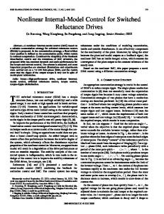
Fig. 1. Naval Combat Survivability (NCS) testbed located at Purdue University. From the left to right: power supply, dc systems (converter module, inverter module, and load bank), synchronous generator with brushless exciter/voltage regulator, pulsed-power load, and induction machine propulsor.

values for resistors, inductors, and capacitors of a switching regulator. These works, while useful, does not focus on the control design problems. Another example of the use of EAs is to determine switching law of an inverter fed by a constant dc source [12]. Herein, the objective is to minimize the error between the actual inductor current and the reference signal. Although this work provides a novel application of EA, it does not provide general switching strategy for common inverter usage. In [13], the authors proposed a multiobjective approach to minimize the size while maximizing the performance of a power converter. Additional examples of the application of EAs in power electronics are set forth in [14]–[19]. Therein the EAs are used to perform worst-case analysis of a power electronic system [14], to design a motor drive regulator [15], to tune an LCL filter [16], to identify unknown parameters for a fluorescent lamp model [17], and to design a sliding-mode based motor controller [18]. Finally, a co-evolutionary computing technique is proposed in [19] to design power electronics regulator similar to [11]. Although there are many examples on the use of evolutionary computing in power electronics, the use of EAs in the design of classical power electronics control using OTDPM has been lacking. Herein, the OTDPM method is used for the control design of a power electronic based power distribution system. Such systems are capable of achieving nearly perfect output voltage and current regulation and nearly instantaneous reconfiguration capabilities [20]. Unfortunately, they are also susceptible to negative impedance instabilities which make the control design critical [21]. Issues addressed herein include: 1) appropriate metrics; 2) imposition of performance constraints; and 3) recognition of control bandwidth limitations. In this work, a multiobjective evolutionary optimization [22] is used to explore the tradeoff between system performance and control effort. For power electronics systems, as the control effort becomes more significant (in terms of its high frequency components), the control design potentially becomes more problematic in terms of effective hardware implementation. Thus, this aspect of the control design is critical. Other important features of the proposed design process include 1) the incorporation of operational limits to prevent overvoltages and overcurrents, 2) the use of a complex multievent scenario to prevent the control design from being overly tuned to a specific event, and 3) effective treatment of the fact that some sets of parameter gains will result in an unstable system whereupon the OTDPM cannot be evaluated.

The specific system considered to demonstrate the proposed concepts is a land-based reduced-scale hardware test system known as the Naval Combat Survivability (NCS) Testbed [23]. The system includes three rotating machines and fourteen power converters. The system model has 73 states. The paper is organized as follows. A description of the NCS testbed is set forth in Section II. In Section III, performance metrics and constraints are addressed. Section IV presents the design problem as an optimization process using EA. A discussion of the results and the conclusion from this work complete the paper.

II. NAVAL COMBAT SURVIVABILITY (NCS) TESTBED The NCS testbed is a reduced-scale test system that represents three-zonal power distribution system of a notional electric warhip system as shown in Figs. 1 and 2. The ac part of the testbed includes a 560-V l-l 59 kW synchronous generator (SG) with a brushless exciter/voltage regulator (EVR), a 40-kW propulsion drive (PD) feeding an induction machine (IM) propulsor, an 18-kW pulsed power (PP) load, and a 15-kW power supply (PS 1) which feeds the 500-V dc port bus of the dc distribution system. A 480-V l-l utility supplies a second power supply (PS 2), which provides power to the starboard bus. In this work, the focus is directed towards the dc distribution system. In addition to the two power supplies already discussed, the dc distribution system consists of six dc-dc converter modules (CM 1 through CM 6) which step the dc voltage from 500 V to 400 V. As can be seen, two CMs feed every inverter module (InV 1 through InV 3) through a pair of auctioneering diodes. Each InV converts power from 400 V dc to 230 V l-l ac, which is the form required by the load banks (LB 1 through LB 3). The redundant topology of the testbed, along with appropriate controls, provides system robustness. When one of the PS fails or a distribution bus is lost, then the other bus can provide the transfer of system loads without service interruption. Faults between the CM and auctioneering diode are restrained by the CM current limit. Meanwhile, the alternate CM provides bump-less load transfer. Internal component level faults are mitigated by the CM controls. A description of the primary dc power system components follows. Additional information on the testbed is set forth in [23].

CHAN et al.: EVOLUTIONARY OPTIMIZATION OF POWER ELECTRONICS BASED POWER SYSTEMS

1909

Fig. 2. One-line diagram of the NCS testbed.

Fig. 3. Power supply (PS).

Fig. 5. PI control with integrator anti-windup.

Fig. 6. Current derivative feedback.

Fig. 4. Commanded output voltage generator.

A. Power Supply (PS) The PS consists of a transformer, a three-phase controlled rectifier, and a low pass filter as shown in Fig. 3. In the case of a three-phase controlled rectifier, the thyristors conduct when they are forward biased and the gating signal, delayed by firing angle , is present. The regulatory controller of the PS is set forth in [24]. First the nominal output voltage is slew-rate limited and scaled to provide short circuit protection as shown in Fig. 4. Fig. 5 depicts the

PI control block with integrator anti-windup. It also includes an inductor current forward path. Fig. 6 depicts the derivative control block which is based on an approximate average-value of the inductor current. It can be shown mathematically that this control block yields the same expression as a derivative operator without actually differentiating the components. Finally, the delay angle is produced in accordance with the diagram shown in Fig. 7. In this work, and denote the filtered values for the output voltage and inductor current respectively. The parameters of the PS are listed in the Appendix. The PS dynamics may be expressed as (1)

1910

IEEE TRANSACTIONS ON POWER ELECTRONICS, VOL. 23, NO. 4, JULY 2008

Fig. 7. Firing angle generator.

Fig. 9. Nonlinear stabilizing controller.

Fig. 10. PI Control with integrator anti-windup. Fig. 8. DC–dc converter (CM).

and (2) where (3) (4) and (5) In (1)–(5), denotes the rms l-n amplitude of the ac input and is the commutating inductance of the transformer as seen by and are positive quantities the secondary. Note that due to the nature of the thyristors and the use of electrolytic capacitors. Interested readers are referred to [25, Chapter 11] for the derivation of the average value model of the PS. In this work, a floating point digital signal processor (DSP) is utilized and hence control bandwidth limitation must be imposed. The gating signal delay is updated discretely at the frequency of 360 Hz to simulate the actual hardware implementation. B. Converter Module (CM) The one line diagram of the CM is shown in Fig. 8. This model considers an input capacitor and an LC filter on the output. All of the capacitors and inductor are shown with equivalent series resistances (ESR) to better represent the actual components. The CM controls consist of two parts. The first part will be referred to as the supervisory control, depicted in [26, Fig. 3.19, Fig.3.20]. It monitors the voltage on the input side of the CM and the user provided on/off command. Based on these values, the supervisory control will enable or disable the device. In this 1 1 denotes that the CM is safe to start work, (operate).

Fig. 11. Inductor current feed-forward.

When it is safe to operate, the performance of the CM is regulated by the second part of the control. Thus it is referred as the regulatory control. Its inputs are the filtered output voltage , filtered inductor current , and a slew rate limited refer. The output of the regulatory control ence output voltage is the commanded inductor current . The nonlinear stabilizing control depicted in Fig. 9 allows input voltage disturbances that fall within a specified frequency range to partially propagate to expressed as the output, with (6) Fig. 10 shows the PI control that includes an output current feed-forward loop and an integrator anti-windup as well as a droop compensation loop for current distribution with multiple CMs. An inductor current feed-forward loop, depicted in Fig. 11, completes the regulatory control. The CM parameters are listed in the Appendix. In terms of an average value model, the capacitor input voltage dynamic is expressed as (7) where (8)

CHAN et al.: EVOLUTIONARY OPTIMIZATION OF POWER ELECTRONICS BASED POWER SYSTEMS

1911

Fig. 13. Simplified dc distribution test bed.

Fig. 12. Inverter module/load bank seen as a constant power load.

In (8), denotes the duty cycle; the ratio of the time the transistor is on to the cycle time. Similarly, the inductor current and output capacitor are governed by

TABLE I SIMULATION SCENARIO

(9) and (10) where . Similar to the PS model, and are positive quantities due to the nature of the semiconductor and the use of electrolytic capacitors. The CM control does not explicitly formulate the duty cycle used extensively in the average value model. For the signal purpose of average value modeling the duty cycle is approximated as (11) . is updated at the rate of 4 Similar to the PS, the duty cycle kHz to represent the hardware implementation. C. Inverter Module/Load Bank (InV/LB) The InV tightly regulates the output voltage to the loads. As such, the combination of an InV and a LB can be represented by the InV input capacitor in parallel with a constant power load as shown in Fig. 12. The InV/LB has a supervisory control similar to that of the CM. Parameters of the InV/LB are listed in the Appendix.

utilized. Since the reduced system must also closely resemble the original system, an appropriate scaling of the currents is required [26]. In particular, the current coming out of the power supply is taken to be three times that going into the CM (since each PS nominally supplies three CMs). The power supply is assumed to be fed by a known (but varying) source. B. Operating Scenario In order to evaluate a time domain based metric, it is necessary to define an operating scenario over which that metric is to be evaluated. In the case of a power electronics based power system, it is appropriate to define a rather complex scenario which covers many of the conditions seen in practice including step load increases, step load shedding events, and a drop in one of the distribution busses. The scenario must be event rich and thoroughly stress the system. If the scenario is too simple, it may result in a design which is overly tuned to a specific event and does not yield good overall performance. The operating scenario used herein is outlined in Table I. In addition to the events listed, the ac input voltages to the PS is subjected to a 5% variation in magnitude at a frequency of 0.4 Hz during the sequence.

III. SYSTEM ASSESSMENT In this section, the issue of system assessment is addressed. This has three parts—the formulation of time-domain simulation, a definition of the operating scenario, and finally a formal definition of the performance metric to be used in the assessment of system performance.

C. Performance Constraints For this design, over and under voltage are not tolerated. Thus, constraints are introduced to prevent these from occurring. To this end, over and under voltage error terms for each bus are defined as

A. Reduced Scope Simulation The use of evolutionary optimization methods entails the use of many 10 10 evaluations of the performance metrics. Thus the system model must be computationally efficient. To decrease computation time, a reduced system, which consists of two PS, two CMs, a single InV/LB as depicted in Fig. 13, is

(12)

(13)

1912

IEEE TRANSACTIONS ON POWER ELECTRONICS, VOL. 23, NO. 4, JULY 2008

Fig. 14. Responsibility signals.

where ' for the port bus, “ ” for the starboard bus, and and denote the “ ” for the zonal bus. In (12) and (13), upper and lower limit of allowed voltage range. is a logical “responsible” signal. In particular, under some conditions, it is physically impossible for the control to avoid under-voltage, such as during startup. Therefore, under-voltage conditions are only conditionally penalized when the controller is deemed “responsible” for avoiding those conditions. Fig. 14 depicts respon, , and . Notice that when PS 1 is turned sible signals off, it is no longer responsible for holding its level. Using the error signals in (12) and (13), a constraint function may be formed as

stays within the permitted boundary, it is evaluated based on the amount of oscillation. To quantify this measure, the bus voltage is first filtered through a high-pass filter defined by (16) ' for the port bus, “ ” for the starboard bus, where again and “ ” for the zonal bus. Next, the filtered component is integrated over the period of simulation and then averaged to obtain an oscillation metric

(14)

(17)

where (15) In (15), “ ” may be “ ” or “ .” The “6” in (14) is the number of constraints. With these definitions, a constraint value 0 implies that all constraints have been met. A constraint value of less than 0 implies that one or more constraints have not been met. Note that the closer becomes to 0, the closer the system comes to satisfying all constraints. D. Performance Metrics If the bus voltage is within the desired limits, its value is not critical. However, it is desired to avoid oscillatory behavior as this increases losses in the capacitors, and may indicate instability in the form of limit cycles. Thus, if the bus voltage

An average oscillation metric for the busses is defined as

(18) It is desired to minimize this metric. E. Control Effort Each PS and CM receives a control signal from its correand for sponding regulatory controller; more specifically PS 1 and PS 2, and for CM 1 and CM 4. Similar to the bus performance metric, these control signals are filtered through a high-pass filter, shown as (19)

CHAN et al.: EVOLUTIONARY OPTIMIZATION OF POWER ELECTRONICS BASED POWER SYSTEMS

1913

B. Fitness Functions

TABLE II GENE DESCRIPTIONS

where is , , , or . Next the filtered value is integrated over the period of simulation and averaged to obtain the control effort metric (20)

is the responsibility signal associated with signal In (20), . For example, in the case is then is . An average control effort metric is defined as (21)

IV. EVOLUTIONARY ALGORITHM In this section, the design problems are formulated as an optimization problem which will be solved using an evolutionary algorithm [27]. The EA code used is Matlab based Genetic Optimization System Engineering Tool (GOSET 2.3), a freeware code developed under Office of Naval Research Support and available at [28]. The default algorithms and parameters were used, with the exceptions that the number individuals and generations are increased to be 450 and 500, respectively. In order to facilitate a large number of time-domain simulations required, a cluster computer was used [29]. The optimization process consumed approximately 11.5 h using 70 processors. Evolutionary algorithm entails formally identifying the design space and defining a fitness function. These issues are addressed below. A. Design Space In this section, parameters of interest are represented as genes on chromosomes. These parameters include control gains and integrator time constants. Table II lists the genes as EA parameters where genes 1 through 6 are CM control parameters and genes 7 through 10 are PS control parameters. All of these genes are continuous (encoded as real numbers) and of logarithmic type (the normalized gene value is formed by mapping the logarithm of the parameter value to the interval [0,1]). Readers are referred to [28] for detailed information on the gene type. As each chromosome set is related to specific control parameters, different chromosome set represents different control system.

There are several considerations which must be taken into account in the construction of a fitness function. First is the selection of the performance metrics. The fitness function should be constructed such that its maximization (in a single or multiobjective sense) should lead to improvement in the performance metrics. In this paper, the first objective function is associated with the system performance, where the performance is inversely proportional to the oscillation metric. The second objective function is formulated to address the issue of control effort. As mentioned previously, as the control effort becomes more significant (higher bandwidth), it becomes problematic in hardware implementation. A second consideration in the construction of the fitness function is that its maximization should lead to all design constraints being satisfied. Further, it is highly beneficial if the fitness function can be constructed so that if constraints are not met, the fitness will improve as constraints become closer to being met, in order to help guide the evolution. A third property that the fitness function should have when utilizing OTDPM objectives is related to the fact that for some values of parameters it is entirely possible that the control design will be unstable, so that the OTDPM cannot be evaluated. The fitness function should also be constructed so that the evolution will first guide the population to a stable control. Applying these general principles to the problem at hand, the time domain simulation used to evaluate the performance metrics attempts to simulate the system performance over a time . However, for some sets of parameters this will span not be possible because the simulation will terminate prior to if the model is unstable for a certain set of parameters. In the simulation used herein such an event is flagged when either or both port and starboard bus voltages leaves the range 400–600 V or when the zonal voltage leaves the range 375–520 V. Let denote the time at which such an event occurs and the simulation exits. With this caveat, the following objective 1 fitness function is proposed: if if otherwise.

(22)

With this objective function, a fitness value from 7 to 6 indicates the premature termination of the simulation. However, increase fitness. Fitness parameter changes that increase values from 6 to 0 indicate it was possible to completely determine system performance; however one or more constraints have not been met. As the fitness increases, the constraints become closer to being met. Finally, fitness values greater than 0 indicated that the simulation was able to complete, and that all constraints have been met. In this case, parameter values with higher fitness indicate a lower oscillation metric. The second fitness function may be similarly expressed if if otherwise.

(23)

1914

IEEE TRANSACTIONS ON POWER ELECTRONICS, VOL. 23, NO. 4, JULY 2008

Fig. 16. Port side distribution bus voltages. Fig. 15. Pareto-optimal front of the nondominated solutions.

This function is quite similar to the first; however, if the simulation is able to complete, and all constraints are met, maximization of causes the control effort to be minimized. While the fitness function formulations in (22) and (23) were found to work well, other formulations are possible. Suppose one desires to minimize an error signal . Since the EAs are generally posed to maximize the objective, the fitness function 1 or , where the former may be formulated as has been chosen in this work. In a single-objective optimization using tournament selection, the choice is arbitrary. In the case of multiobjective optimization, the choice may have a minor impact on convergence. If the designers prefer the latter form, then (22) and (23) may be formulated as if if otherwise

(24)

if if otherwise

(25)

Fig. 17. Starboard side distribution bus voltages.

and

where 0 denote penalties sufficiently larger than the error terms. In (24) and (25), it should be noted that if , . The advantage of the proposed approach (22), it falls that (23) over (24), (25) is that there is no need to identify suitable and . values for V. RESULTS A. EA Optimization Results The multiobjective EA optimization yields a set of solutions providing the tradeoff between system performance and control effort. A multiobjective EA shows the results in the form of a Pareto-optimal front. Fig. 15 depicts only the nondominated solutions within the Pareto-optimal front. The Pareto-optimal front offers a family of solutions as oppose to a single solution in a single objective optimization problem. In simulation, three sets of parameters are chosen; one

with the minimum control effort, one with maximum control effort, and one arbitrarily chosen in between. In addition, a set of baseline parameters is used for reference. This baseline was designed using classical methods (in particular pole placement using linearized models as well as some trial-and-error tuning [30], [31]) and was performed prior to the author’s conception of this work, thus eliminating psychological bias. These parameters are documented in [23]. B. Simulation Results Shown herein are the simulation results corresponding to the three sets of EA parameters and the baseline parameters. Figs. 16–18 depict the port, starboard, and zonal bus voltages under the four chosen sets of control parameters for the operating scenario discussed in Table I. The PS, CM, and InV are turned on sequentially after ensuring the input voltage to each device has reached steady state. The load to the system is increased gradually before one of the PS is turned off to simulate a fault in one of the distribution busses. In these figures, it can be seen that the performances of the port and starboard busses

CHAN et al.: EVOLUTIONARY OPTIMIZATION OF POWER ELECTRONICS BASED POWER SYSTEMS

Fig. 18. Zonal bus voltages.

1915

Fig. 20. Commanded inductor current i

for CM 4.

TABLE III EA RESULTS

TABLE IV HARDWARE SCENARIO

Fig. 19. Firing angle  for PS 2.

are improved relative to the baseline design while the dc zonal voltages are nearly identical. and for Figs. 19 and 20 below depict the control signal PS 2 and CM 4, respectively. Herein, readers may observe that the control signals become more aggressive as the control effort increases. C. Hardware Validation From the three sets of parameters simulated, the set with minimum control effort is chosen to be used in hardware validation. This set of parameters is listed in Table III. The scenario for hardware validation is somewhat different from that used to train and is described in Table IV. Perhaps the most significant difference is that the ac bus magnitude is no longer a stiff source with a varying magnitude, but instead the voltage is obtained from the generator/voltage regulator. Figs. 21–23 depict the performance of the port, starboard, and 27 s. zonal bus voltages. PS 1 is turned off at approximately The CMs on the port side shut down when the input voltage drops below 435 V. At this point, the only discharge path for the PS is through the leakage resistance, thus the voltage decays

slowly after the sharp initial drop. As mentioned previously, the topology of the testbed is designed for system robustness. Thus when one of the distribution busses is lost, the other bus can provide transfer of system loads without service interruptions. In these figures, solid traces indicate hardware measurements, while dotted lines indicate simulation results. Readers may observe that these two traces are nearly identical, except in Fig. 22. Herein, the simulation voltage drop is more significant than the hardware measurement due to lighter aggregate loads during hardware experimentation. Throughout the scenario, the performance of the control system in regulating the starboard and zonal busses is quiet acceptable. In the sense the proposed use of OTDPM method for the selection of the control system parameters would seem to be successful. This in turn suggests that if the effort to develop a system simulation is to be made, that simulation can be used as the principle design tool for the control rather than being restricted in use of the validation of control parameters obtained using some other methods. VI. CONCLUSION The conclusion of this work is to suggest that OTDPM is a viable method to select control system parameters. In situations

1916

IEEE TRANSACTIONS ON POWER ELECTRONICS, VOL. 23, NO. 4, JULY 2008

in OTDPM designs are related to appropriate representation of hardware limitations such as control bandwidth constraints. APPENDIX

Fig. 21. Hardware measurement of port bus voltage.

0.82 for PS 1, 0.97 The PS parameters are: for PS 2, 14.0 mH, 0.98 , 4.4 mF, 0.62 , and 662.0 H, filter time constants 0.15 ms and 0.15 ms, 500 V, maximum and minimum rate of increase 500 V/s and 2 MV/s, respectively, slew rate limiter time 0.1 ms, short circuit current protection level constant 55 A, and threshold current level 35 A. The cosine of the firing angle is bounded between 1.0 and 0.9. 449.0 F, 1.12 , The CM parameters are: 0.99 mH, 0.12 , 447 F, and 0.128 . The control parameters: 420 V, 500 V/s, 2 MV/s, with the droop set1.6 , input filter time constants 0.15 ms, ting 0.15 ms, 1.5 ms. The inductor current feedback is limited to 2 A while the inductor current is 20 A. The supervisory control parameters limited to 450(435) V and 550(575) V as the are: minimum and maximum to activate (operate), respectively. 590 F and The InV/LB parameters are 0.127 . The supervisory control parameters are: 360(340) V and 460(480) V minimum and maximum to activate (operate), respectively. REFERENCES

Fig. 22. Hardware measurement of starboard bus voltage.

Fig. 23. Hardware measurement of zonal bus voltage.

where a time domain simulation is to be developed, OTDPM allows the simulation to be used as the principle design tool instead of being restricted in use to a design check. Challenges

[1] A. El dessouky and M. Tarbouchi, “Fuzzy model reference learning control of induction motor via genetic algorithm,” in Proc. 27th Annu. Conf. IEEE Ind. Electron. Soc., Nov. 29, 2001, pp. 2038–2043. [2] J. G. Juang, K. C. Chin, and J. Z. Chio, “Intelligent automatic landing system using fuzzy neural networks and genetic algorithm,” in Proc. Amer. Control Conf., Jun. 30, 2004, pp. 5790–5795. [3] R. J. Wai and C. H. Tu, “Design of total sliding-mode based genetic algorithm control for hybrid resonant-driven linear piezoelectric ceramic motor,” IEEE Trans. Power Electron., vol. 22, no. 2, pp. 563–575, Mar. 2007. [4] Y. Qiu, M. Xu, J. Sun, and F. C. Lee, “High-frequency modeling for the nonlinearities in buck-converters,” in Proc. APEC’06, Mar. 2006, pp. 1197–1203. [5] T. Ota and S. Omatu, “Tuning of the PID control gains by GA,” in Proc. IEEE Conf. Emerging Tech. Factory Autom., 1996, vol. 1, pp. 272–274. [6] J.-C. Shen, “New tuning method for PID controller,” in Proc. IEEE Int. Conf. Control Appl., 2001, pp. 459–464. [7] A. Dupuis, M. Ghribi, and A. Kaddouri, “Multiloop PI tuning using a multiobjective genetic algorithm,” in Proc. IEEE Conf. Ind. Tech., 2004, vol. 3, pp. 1505–1510. [8] D. P. Kwok and F. Sheng, “Genetic algorithm and simulated annealing for optimal robot arm PID control,” in Proc. IEEE Cond. Evol. Comp., 1994, vol. 2, pp. 707–713. [9] A. Popov, A. Farag, and H. Werner, “Tuning of a PID controller using a multiobjective optimization technique applied to a neutralization plant,” in Proc. IEEE Conf. Decision Control, 2005, pp. 7139–7143. [10] P. Zanchetta, M. Summer, F. Cupertino, M. Marinelli, and E. Mininno, “On-line and off-line control design in power electronics and drives using genetic algorithm,” in Proc. IEEE Ind. Appl. Conf., 2004, vol. 2, pp. 864–871. [11] J. Zhang, H. S. H. Chung, W.-L. Lo, S. Y. Hui, and A. K.-M. Wu, “Implementation of a decoupled optimization technique for design of switching regulators using genetic algorithm,” IEEE Trans. Power Electron., vol. 16, no. 6, pp. 752–763, Nov. 2001. [12] M. J. Schutten and D. A. Torrey, “Genetic algorithms for control of power converters,” in Proc. IEEE Power Electron. Spec., 1995, vol. 2, pp. 1321–1326.

CHAN et al.: EVOLUTIONARY OPTIMIZATION OF POWER ELECTRONICS BASED POWER SYSTEMS

[13] D. V. Malyna, J. L. Duarte, M. A. M. Hendrix, and F. B. M. van Horck, “Multiobjective optimization of power converters using genetic algorithm,” in Proc. Int. Symp. Power Electron., Elect. Drives, Autom., Motion, 2006, pp. 713–714. [14] T. Kato, K. Inoue, and K. Nishimae, “Worst-case tolerance analysis for a power electronic system by modified genetic algorithms,” in Proc. Power Electron. Motion Control Conf., 2006, vol. 2, pp. 1–5. [15] B. Cassimere, S. D. Sudhoff, D. C. Aliprantis, and M. D. Swinney, “Time-domain design of motor drive current regulators using genetic algorithms,” in Proc. IEEE Int. Conf. Elect. Mach. Drives, 2005, pp. 1737–1743. [16] M. Liserre, A. Dell’Aquila, and F. Blaabjerg, “Genetic algorithm-based design of the active damping for an LCL-filter three-phase active rectifier,” IEEE. Trans. Power Electron., vol. 19, no. 1, pp. 76–86, Jan. 2004. [17] W. Yan, E. Tam, and S. Y. Hui, “A semi-theoretical fluorescent lamp model for time-domain transient and steady-state simulations,” IEEE Trans. Power Electron., vol. 22, no. 6, pp. 2106–2115, Nov. 2007. [18] W. Rong-Jong and T. Ching-Hsiang, “Design of total sliding-modebased genetic algorithm control for hybrid resonant-driven linear piezoelectric ceramic motor,” IEEE Trans. Power Electron., vol. 22, no. 2, pp. 563–575, Mar. 2007. [19] J. Zhang, A. K. M. Wu, and H. S. H. Chung, “On the use of pseudo-coevolutionary genetic algorithms with adaptive migration for design of power electronics regulators,” in Proc. IEEE Int. Symp. Circuits Syst., 2001, vol. 2, pp. 297–300. [20] S. D. Sudhoff, S. F. Glover, S. H. Zak, S. D. Pekarek, E. L. Zivi, D. E. Delisle, and D. Clayton, “Stability analysis methodologies for dc power distribution systems,” presented at the 13th International Ship Control Systems Symposium, Orlando, FL, 2003. [21] R. D. Middlebrook, “Input filter considerations in design and application of switching regulators,” in Proc. IEEE Industry Application Society Conference (IASAM), 1976, pp. 91–107. [22] K. Deb, Multiobjective Optimization Using Evolutionary Algorithms. New York: Wiley, 2002. [23] S. D. Pekarek, J. Tichenor, S. D. Sudhoff, J. D. Sauer, D. E. Delisle, and E. J. Zivi, “Overview of a naval combat survivability program,” in Proc. 13th Int. Ship Control Syst. Symp., Orlando, FL, 2003, pp. 1–10. [24] A. M. Cramer, R. R. Chan, S. D. Sudhoff, Y. Lee, M. R. Suuprenant, N. S. Tyler, E. L. Zivi, and R. A. Youngs, “Modeling and simulation of an electric warship integrated engineering plant,” presented at the SAE Power Syst. Conf., Nov. 2006. [25] P. C. Krause, O. Wasynczuk, and S. D. Sudhoff, Analysis of Electric Machinery and Drive Systems, 2nd ed. New York: Wiley, 2002. [26] A. Doyle, “Time domain control design of a dc–dc converter module with application to zonal dc power distribution,” M.S. thesis, Dept. Elect. Comp. Eng, Purdue Univ., W. Lafayette, IN, 2005. [27] D. E. Goldberg, Genetic Algorithms in Search, Optimization, and Machine Learning. New York: Addison-Wesley, 1989. [28] “Genetic Optimization System Engineering Tool (GOSET) for Use With MATLAB,” ver. 2.2, School Elect. Comp. Eng., Purdue Univ., West Lafayette, IN, 2005. [29] School of Electrical and Computer Engineering, Purdue Univ., in Proc. Annu. Res. Summary, West Lafayette, IN, Jun. 2003 [Online]. Available: https://engineering.purdue.edu/ECE/Research/ARS/ARS2003/ars2003.pdf, Purdue University [30] A. R. Oliva, S. S. Ang, and G. E. Bortolotto, “Digital control of a voltage-mode synchronous buck converter,” IEEE Trans. Power Electron., vol. 21, no. 1, pp. 157–163, Jan. 2006. [31] K. Kiyong and R. C. Schaefer, “Tuning a PID controller for a digital excitation control system,” IEEE Trans. Ind. Appl., vol. 41, no. 2, pp. 485–492, Mar./Apr. 2005.

1917

Ricky R. Chan (S’06) received the B.S. and M.S. degrees in electrical engineering from Purdue University, West Lafayette, IN, in 2003 and 2005, respectively, where he is currently pursuing the Ph.D. degree in electrical engineering. His research interest includes power electronic converters, power systems, and evolutionary computing.

Yonggon Lee received the B.S. degree in electrical engineering from Yonsei University, Seoul, Korea, in 1994, the M.S. degree in electrical engineering from the University of Michigan, Ann Arbor, in 1997, and the Ph.D. degree in electrical engineering from Purdue University, West Lafayette, IN, in 2003. Currently, he is an Assistant Research Professor in the Weapons and Systems Engineering Department, Unites States of Naval Academy, Annapolis, MD. His research interests include genetic algorithms, neural fuzzy systems, and adaptive robust control.

Scott D. Sudhoff (F’08) received the B.S. (with highest distinction), M.S., and Ph.D. degrees in electrical engineering from Purdue University, West Lafayette, IN, in 1988, 1989, and 1991, respectively. From 1991 to 1993, he served as a consultant for P.C. Krause and Associates in aerospace power and actuation systems. From 1993 to 1997, he served as a faculty member at the University of Missouri-Rolla, and in 1997 he joined the faculty of Purdue University where he currently holds the rank of Full Professor. He has published over 100 papers in these areas, including six prize papers. His interests include electric machinery, power electronics, marine and aerospace power systems, applied control, and evolutionary computing. Much of his current research focuses on genetic algorithms and their application to power electronic converter and electric machine design.

Edwin L. Zivi (M’02) received a B.S. degree in engineering science and mechanics at the Virginia Polytechnic Institute and State University (Virginia Tech), Blacksburg, in 1975 and the M.S. and Ph.D. degrees in mechanical engineering from the University of Maryland, College Park, in 1983 and 1989, respectively. He is presently an Associate Professor of Systems Engineering at the U. S. Naval Academy, Annapolis, MD. Prior to 1998, he was a Senior Research Engineer and Technical Advisor at the U. S. Naval Surface Warfare Center (NSWC), Annapolis, MD. His research focuses on the integration of survivable naval automation systems with advanced shipboard engineering and damage control systems.