Evolving HMMs For Network Anomaly Detection

Evolving HMMs For Network Anomaly Detection – Learning Through Evolutionary Computation Juan J. Flores Division de Estudios de Posgrado Universidad Michoacana Morelia, Mexico [email protected]

Anastacio Antolino Division de Estudios de Posgrado Universidad Michoacana Morelia, Mexico [email protected]

Abstract—This paper reports the results of a system that performs network anomaly detection through the use of Hidden Markov Models (HMMs). The HMMs used to detect anomalies are designed and trained using Genetic Algorithms (GAs). The use of GAs helps automating the use of HMMs, by liberating users from the need of statistical knowledge, assumed by software that trains HMMs from data. The number of states, connections and weights, and probability distributions of states are determined by the GA. Results are compared to those obtained with the Baum-Welch algorithm, proving that in all cases that we tested GA outperforms Baum-Welch. The best of the evolved HMMs was used to perform anomaly detection in network traffic activity with real data. Keywords-HMMs; GAs; Anomaly Detection; Baum-Welch;

I. I NTRODUCTION Security threats for computer systems have increased immensely which include virus, denial of service, vulnerability break-in, etc. While many security mechanisms have been introduced to undermine those threats, none can completely prevent all of them. Security threats to the computer systems have raised the importance of anomaly detection [1]. Anomaly detection is the process of monitoring the events occurring in a computer system or network and analyzing them for signs of anomaly. Anomaly is defined as attempts to compromise the confidentiality, integrity, availability, or to bypass security mechanism of a computer or network. Hidden Markov Models (HMMs) are based on a probabilistic finite state machine used to model stochastic sequences [2]. HMMs have many applications in signal processing, pattern recognition, speech and gesture recognition, as well as applications to anomaly detection. It is important to mention that in an HMM, the estimation of good model parameters affects the performance of the recognition [3] or detection processes. The HMM parameters can be determined during an iterative process called “training”. The Baum-Welch algorithm [4] is one method applied in setting an HMM’s parameters, but this method has a drawback: being a gradient-based method, it may converges to a local optimum. Global search techniques can be used to optimize an HMM’s parameters. Genetic Algorithms (GAs) are a global

Juan M. Garcia Division de Estudios de Posgrado Universidad Michoacana Morelia, Mexico [email protected]

optimization technique that can be used to optimize an HMM’s parameters [3]. Studies of using GAs to train HMMs are relatively rare, particularly in comparison with the large literature on applying GAs to neural network training [2]. In this paper we present the use of GAs for creation and optimization of an HMM on one step; our system takes a time series as input data and produces a trained HMM, without any human intervention. After that, the HMM model is used for anomaly detection in computer network traffic. Finally, we compare the performance of HMMs created with GA against others trained with the Baum-Welch algorithm. The remainder of the paper is structured as follows: Section II introduces the related HMM theory. Section III describes GAs for readers not familiar with the topic. Section IV defines Anomaly Detection. Section V illustrates the results on comparing HMMs created with GAs against those trained with the Baum-Welch algorithm. Section VI presents our conclusions and future work. II. H IDDEN M ARKOV M ODELS An HMM is a doubly stochastic process with an underlying stochastic process that is not observable, but can only be observed through another set of stochastic processes that produce the sequence of observed symbols. The most common application of HMMs, which are best known for their contribution, is in automatic speech recognition, where HMMs were used to characterize the statistical properties of a signal [4], [5]. Recently, HMMs have been applied to a variety of applications outside of speech recognition, such as bioinformatic, handwriting recognition, pattern recognition in molecular biology, and fault detection. Variants and extentions of HMMs include econometrics, time series, and signal processing [6]. An HMM is formed by a finite number of states connected by transitions, which can generate an observation sequence depending on its transition, and initial probabilities [4]. A Markov Model is hidden because we do not know which state led to each observation.

An HMM is defined, among others, basically by these three parameters: A = {aij } is the state transition probability matrix. B = {bj (k)} is the emission probability matrix, indicating the probability of a specified symbol being emitted given that the system is in a particular state. Π = {π i } is the initial state probability distribution. An HMM can therefore be defined by the triplet [7]:

Table I A C OMPLETE C HROMOSOME FOR E VOLVING HMM S Fitness

Size

Transitions

Parameters

Pi

crossover, and mutation are three main operators of GA, and individuals are the objects upon which those operators work. You can find the general steps of a GA in Zhang et al. [9]. B. A Framework for Evolving an HMM

λ = {A, B, π}

(1)

There are three basic problems of interest that must be solved for the HMMs to be useful in real-world applications: 1) Determine the probability that a given observation sequence had been generated by λ. 2) Determine the highest-probability state sequence for a given observation sequence and a λ. 3) Adjust or re-estimate the model’s parameters λ. HMMs deal with the problems described above, under a probabilistic or statistical framework. HMMs offer the advantages of having strong and powerful statistical foundations and being computationally efficient to develop and evaluate due to the existence of established training algorithms. But one disadvantage of using HMMs is the need for an a-priori notion of the model topology. That is, in order to build an HMM we must first decide how many states the model will contain and what transitions among states will be allowed. Once a model structure has been designed, the transition and emission parameters need to be estimated from training data. The Baum-Welch algorithm is used to train model parameters. Baum-Welch training suffers from the fact that it finds local optima, and is thus sensitive to initial parameters settings. For further information on HMMs and the BaumWelch algorithm, please see [4]. III. G ENETIC A LGORITHMS HMMs parameters are determined during an iterative process called “training”. One of the conventional methods applied in HMM model parameter values is the BaumWelch algorithm [4]. One drawback of this method is that it converges to a local optimum. Genetic Algorithms (GA) is a global optimization technique that can be used to optimize the HMM parameters [3], [8]. A. Basic Concepts GAs simulate evolution phenomena of nature. The possible solution is encoded into a vector; elements of the chromosome vector are called genes. Through continually calculating the fitness of each chromosome, the best chromosome is selected and the optimization solution is obtained [9]. The GA is a robust general purpose optimization technique, which evolves a population of solutions [3]. Selection,

In this subsection we propose a framework for building and evolving an HMM’s structure and parameters. The evolution process consists of: • A population of chromosomes. One chromosome is constituted as shown in Table I. These genes are described as: 1) Fitness. This is its fitness evaluation, after being evaluated by the objective function (see Equation 2). P (O|λ) =

N X

αT (i),

(2)

i=1

Where αT (i) represents the sum of the terminal Forward variables [4]. 2) Size. It is a value that indicates the number of states of the HMM. 3) Transitions. This set of genes has the probability transitions among the states of the HMM. 4) Parameters. This set of genes contains the Mean and Variance of a Gaussian distribution function of each state in the HMM. 5) Pi. The last set of genes represents the probability of state Si to start at time t = 1. Where the chromosomes are the encoded form of the potential solution. Initially, the population is generated randomly and the fitness values of all chromosomes are evaluated by calculating the objective function (Equation 2), where P (O|λ) [4] represents the probability that the observation sequence had been generated by model λ (Equation 1). • After the initialization of the population pool, the GA evolution cycle begins. At the beginning of each generation, the mating pool is formed by selecting some chromosomes from the population. This pool of chromosomes is used as parents for the genetic operations to generate the offspring. The genetic operators are implicit in our evolutive operators, as we will see later. Each offspring is a complete HMM, so the system calculates how good this model is with respect to the observation sequence; we compute its probability and assign this value as its fitness. That is, the topology with the maximum value of likelihood is considered as the best topology.

At the end of the generation, some chromosomes will be replaced by the offspring, maintaining a population of constant size across generations, preserving offspring and parents with the best fitnesses. • This GA is setup to apply the following evolutive operators: mutParams (mutates parameters values mean and variance), mutTransition (mutates probability values on transition links among states), delTransition (deletes a state transition), addTransition (adds a new state transition), Copy (copies a complete chromosome), addNode (adds a new node to the model), and delNode (deletes a node from the model). This GA builds HMM models ranging from 3 to 15 states. The Mean and Variance are randomly initialized and evolution is driven by mutating the parameters’ magnitude. • The above process is repeated until the cycle gets the maximum number of generations. By emulating the natural selection and genetic operations, this process will hopefully determine the best chromosomes of the highly optimized solutions to the problem. Once GA has finished evolving an HMM, we take the best model of the last generation and use it to determine if a given observation sequence has anomalies or not. Our new statistic model can examine new observation sequences and determine if a time series belongs to this model. That is, if the observations are likely to have been produced by the model. If the observations have a low probability of belonging to the model, it is possible that the sequences present an anomaly. We are for now using a single random variable and analyzing its behavior. The HMM generated and optimized by GAs is a great help to detect statistically anomalous behavior; its function is to detect anomalous behavior and discriminates over a normal one. HMMs focus on statistics-based anomaly detection techniques. We built a statistics-based normal profile and employed statistical tests to determine whether observed activities deviate significantly from the normal model. •

IV. A NOMALY D ETECTION Anomaly detection is performed by detecting changes in the patterns of resources utilization or behavior of the system. Anomaly detection may be performed by building a statistical model that contains metrics derived from system operation and flagging as intrusive any observed metrics that have a statistically significant deviation from the model [1]. In other words, an anomaly detection uses a model of “normal” network behavior to compare to currently observed network behavior. Any behavior that varies from this model is considered a network anomaly and behaviors closely matching the model are considered as “normal”. In general, the normal behavior of a computing system can be characterized by observing its properties over time. The problem of detecting anomalies can be viewed as filtering non-permitted deviations of the characteristic prop-

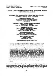
Figure 1.

Network Bandwidth with normal and anomalous behavior

erties in the monitored network system [10]. Anomaly detection can also be defined as the process of identifying malicious behavior that targets a network and its resources [11]. Anomaly detection research is carried out in several application domains, such as monitoring business news, epidemic or bioterrorism detection, intrusion detection, hardware fault detection, network alarm monitoring, fraud detection, etc. The anomaly detection problem involves large volumes of time series data, which has a significant number of entities and activities. The main goal of anomaly detection is to identify as many interesting and rare events as possible with minimum delay and the minimum number of false alarms [12]. V. R ESULTS This section presents the results of our proposal and compares them with those obtained using the Baum-Welch learning algorithm. It also presents the results of using HMMs in anomaly detection. In all our experiments we used a time series produced by network bandwidth usage (Figure 1) in our University. These values recorded bandwidth used for our department. HMMs training used this series with 48 values, which corresponds to bandwidth used in kbit/second in two consecutive days. The bandwidth usage values fluctuate between 14.625 and 5964.81 kbit/second. The time series was modified (using random values) to simulate an anomalous behavior; in the presence of a given kind of attack, the bandwidth usage increases. A. HMMs Produced by GAs Our system evolves HMMs using GAs and the data from the bandwidth used, with different number of generations and different population sizes. Table II describes several examples of HMMs evolved with GAs. The second column of Table II, shows each model’s probabilities for the observation sequence. We selected our HMM from these evolved models. We took the model with the highest probability, and used it in our anomaly detection tests.

Table II S EVERAL HMM S E VOLVED BY GA S Num. of States

Population

Num. of Generations

P(O | λ)

5

500

500

7.70688 × 10−103

5

500

250

7.70688 × 10−105

6

250

250

2.52091 × 10−75

6

200

50

7.19032 × 10−98

8

1000

500

1.19399 × 10−88

Figure 3.

Figure 4. Figure 1

•

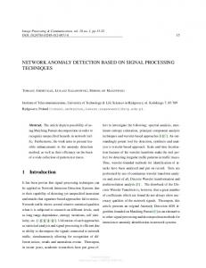
Figure 2.

Evolving an HMM with GAs

•

HMM Evolved by GAs for data in Figure 1

HMM Trained by the Baum-Welch Algorithm for data in

ground knowledge about statistical models. GA does everything, creates and optimizes an HMM based on the time series data and a probabilistic function to qualify that sequence. All this method needs is a time series data, our fitness function (Equation 2), and time for processing the learning method. GA builds an HMM with all the required parameters.

B. Baum-Welch Learning Figure 2 shows how GAs evolve HMMs; each subfigure shows the best individual of corresponding generations. a) Generation 1, produced an HMM with 14 states. b) generation 5, has evolved to 13 states, c) generation 10, HMM has 12 states, d) generation 11, evolved to 11 states, e) in generation 85, has an HMM with 10 states, and f) presents the final HMM evolved with states and transitions. In the last generations, GA has already come to an optimum number of states and focuses on refining the transition probabilities. Figure 3, shows an HMM evolved with GAs. This HMM was evolved based on the observation sequence given by the network bandwidth used in our University. Regarding our results, we observed the following points: •

GA does not assume the user to possess any back-

We took an HMM structure created randomly, and trained it with the Baum-Welch algorithm, obtaining a reestimated HMM. This HMM was trained based on the observation sequence given by the bandwith used (Figure 1). Figure 4 shows the HMM obtained with the Baum-Welch algorithm in 50 iterations. Table III describes our tests and results. We created several HMMs and reestimated their parameters using the BaumWech algorithm, trying to get better probabilities for our models. We started with a 3-state HMM; see the first column of Table III. The second column, labeled P(O | λ), shows the probability for each model, obtained using the Baum-Welch algorithm. In all tests we performed, we applied the BaumWelch algorithm for 50 iterations. Our initial models were built with random values as initial parameters. These HMMs

Table III S EVERAL HMM S T RAINED WITH THE BAUM -W ELCH A LGORITHM Number of States

P(O | λ) 10−123

3

1.8920 ×

4

6.44442 × 10−175

5

3.43836 × 10−137

6

1.07894 × 10−127

7

5.90112 × 10−125

8

1.09739 × 10−119

9

1.22676 × 10−119

10

6.55885 × 10−172

present low probabilities because they try to represent the complete likelihood of all the observation sequence. The Baum-Welch algorithm is a good method for learning using time series data, but its problem is that it converges to a local optimum. Another problem that this algorithm presents, is that users need a previous background or knowledge about HMMs theory and how to build it. The Baum-Welch algorithm’s performance depends a lot on a good set of initial parameters to refine them. That is, if we give it bad starting parameters, the method may diverge. From our experiments, we realize that the Baum-Welch algorithm needs for its proper usage: • An initial number of states. • An initial starting point (an estimate for transition and starting point probabilities). • A Probability Distribution function for each state. • And needs the expertise of the users. As a conclusion, we noted that the models that we created and trained with the Baum-Welch algorithm did not perform as well as any of the HMM models created with GA, where the probability of the best model is 2.5209 x 10−75 with 6 states (see Table II). C. Anomaly Detection Table IV describes the results of applying HMMs, trained with the Baum-Welch algorithm, to detecting anomalous behavior. Our experiments’ setup is the following: given an observation sequence, the trained HMM analyzes a time window of data and determines the probability of that sequence having been generated by the model. Our time window moves to the next item in the time series, which is also verified by the HMM. The process continues until the whole test time series is traversed and tested. The window sizes we tested were 3, 4, 5, and 6. All these probabilities, generated by the sliding time window and the HMM, were compared with our probability threshold and then analyzed to determine if an anomaly exists or not. We do not report all that information for the lack of space. Instead, we report the percentages of hits, false positives, and

Table IV R ESULTS OF A NOMALY D ETECTION USING AN HMM T RAINED WITH BAUM -W ELCH ALGORITHM Window Size 3 4 5 6

Hits 57 60 59 65

% False Positives 43 40 41 35

False Negatives 0 0 0 0

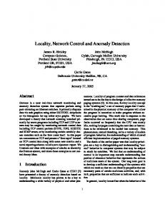
Figure 5. Probability threshold between Normal and Abnormal Behaviors Table V R ESULTS OF A NOMALY D ETECTION USING AN HMM E VOLVED WITH GA S Window Size 3 4 5 6

Hits 89 93 89 84

% False Positives 7 2 4 5

False Negatives 4 5 7 11

false negatives. Table IV shows these results. Table V shows the results from an HMM evolved through GA used in anomaly detection. Our experiments’ setup is the same as mentioned above. We took the same time series and applied the same windows sizes, following the same steps. All these probabilities, generated by the sliding time window and the HMM evolved, were also compared with our probability threshold (see Figure 5), to determine if an anomaly exists or not. We also reported the percentages of hits, false positives, and false negatives. Table V shows these results. Figure 5 shows the probabilities obtained through the application of the HMM to the sliding window data for normal and anomalous behaviours. A probability threshold is set, which helps to determine if an anomalous behavior exists in the time series. The method we are using to analyze and determine possible anomalies, is comparing the probability generated by a time window of the time series, with the probability threshold. If this value is lower than our probability threshold, we flagged the window as anomalous behavior. Our experiments report the best result with a window

size of 6, using an HMM trained with the Baum-Welch algorithm, with a 65% of correct detections or hits, 35% of false positives, and 0% of false negatives. The worst result was produced for window size of 3, with 57% of hits, 43% of false positives, and 0% of false negatives. The best result with a window size of 4, using an HMM evolved with AGs, with a 93% of hits, 2% of false positives, and 5% of false negatives detections. The worst result was produced for window size of 6, with 84% of hits, 5% of false positives, and 11% of false negatives. VI. C ONCLUSIONS A ND F UTURE W ORK In this paper, we outlined a framework for evolving HMMs used for anomaly detection. These models generated and optimized by GAs, provide detection capabilities for anomalous behavior. They are capable of distinguishing between normal and abnormal behaviors. Our experiments show that Hidden Markov Models do well, 93%, over anomaly detection. All models were produced by means of GA, without the need of human intervention at all. The GA determines the size of the HMM, the probability distributions on each state, and the transition probabilities among pairs of states. Forthcoming experiments include using parallelizing the design and evolutionary process. We hope in the near future, to compare our method with some others, like the one used by Warrender et al. [13] and determine how good our system is against others. Finally, we also plan to observe and model several variables to build an HMM. Our work on HMMs is centered around the task of anomaly detection in a network bandwidth usage. The models we described in this paper are built from time series data of bandwidth used, and the models can be deployed by our computer center in a near future. We expect these improvement to contribute to the development of more accurate models for anomaly detection using HMMs. R EFERENCES [1] M. H. Islam and M. Jamil, “Taxonomy of statistical based anomaly detection techniques for intrusion detection,” pp. 270–276, 2005. [2] K.-J. Won, T. Hamelryck, A. Prugel-Bennett, and A. Krogh, “Evolving hidden markov models for protein secondary structure prediction,” Evolutionary Computation, IEEE, vol. 1, pp. 1–18, September 2005. [3] M. Korayem, A. Badr, and I. Farag, “Optimizing hidden markov models using genetic algorithms and artificial immune systems,” Computing and Information Systems, vol. 11, no. 2, 2007. [4] L. R. Rabiner, “A tutorial on hidden markov models and selected applications in speech recognition,” Proceedings of the IEEE, vol. 77, no. 2, February 1989.

[5] L. R. Rabiner and B. H. Juang, “An introduction to hidden markov models,” IEEE ASSP Magazine, 1986. [6] Y. Bengio, “Markovian models for sequential markovian models for sequencial data,” Statistical Science, 1997. [7] P. Nicholl, A. Amira, D. Bouchaffra, and R. H. Perrot, “A statistical multiresolution approach for face recognition using structural hidden markov models,” EURASIP Journal on Advances in Signal Processing, ACM, vol. 2008, p. 13, 2008. [8] P. Bhuriyakorn, P. Punyabukkana, and A. Suchato, “A genetic algorithm-aided hidden markov model topology estimation for phoneme recognition of thai continuous speech,” in Ninth ACIS International Conference on Software Engineering, Artificial Intelligence, Networking and Parallel/Distributed Computing. IEEE, 2008, pp. 475–480. [9] X. Zhang, Y. Wang, and Z. Zhao, “A hybrid speech recognition training method for hmm based on genetic algorithm and baum welch algorithm,” IEEE, pp. 572–572, 2007. [10] D. Dasgupta and H. Brian, “Mobile security agents for network traffic analysis,” IEEE Transactions on Power Systems, vol. 2, no. 332-340, 2001. [11] F. Jemili, M. Zaghdoud, and M. Ben Ahmed, “A framework for an adaptive intrusion detection system using bayesian network,” Intelligence and Security Informatics, IEEE, 2007. [12] S. Singh, W. Donat, K. Pattipati, and P. Willet, “Anomaly detection via feature-aided tracking and hidden markov model,” Aerospace Conference, IEEE, pp. 1–18, March 2007. [13] C. Warrender, S. Forrest, and B. Pearlmutter, “Detecting intrusions using system calls: Alternative data models,” in Security and Privacy, 1999. Proceedings of the 1999 IEEE Symposium on. IEEE, May 1999, pp. 133–145.