Fibonary Spray and Wait Routing in Delay Tolerant ...

International Journal of Electrical and Computer Engineering (IJECE) Vol. 6, No. 6, December 2016, pp. 3205 – 3216 ISSN: 2088-8708, DOI: 10.11591/ijece.v6i6.10361

3205

Fibonary Spray and Wait Routing in Delay Tolerant Networks Priyanka Das1 , Prosenjit Chowdhury2 , Bikash Poudel3 , and Tanmay De4 1

Department of Computer Science & Engineering, NSHM Knowledge Campus Durgapur, India 2 Software Engineer, o9 Solutions, Bangalore, India. 3 Software Engineer, Meru Networks, India 4 Department of Computer Science & Engineering, National Institute of Technology Durgapur, India

Article Info

ABSTRACT

Article history: Received Mar 2, 2016 Revised Aug 18, 2016 Accepted Sep 5, 2016

Although there has been a tremendous rise in places being connected through the Internet or any other network protocol, there still lie areas, which remain out of reach due to various reasons. For all such places the answer is a Delay Tolerant Network (DTN). A DTN is such a network where there is no fixed or predefined route for messages and no such guarantee whatsoever of all messages being correctly routed. DTN can be considered as a superset of networks wherein other networks such as adhoc, mobile, vehicular etc. form the subset. Therefore routing in DTN is a very chancy affair where one has to maximize on the present network scenarios to get any fruitful result other than depending on past information. Also protocols here need to be less complex and not increase the already high nodal overhead. In this paper we propose a new approach, the Fibonary Spray and Wait, which does exactly this. It forwards copies of a message in a modified Binary Spray and Wait manner so that it performs well even in non independent and identically distributed node structure. We have supported our statements with mathematical as well as simulation analysis.

Keyword: Delay Tolerant Network (DTN) fibonary latency delivery ratio

c 2016 Institute of Advanced Engineering and Science. Copyright All rights reserved.

Corresponding Author: Name Priyanka Das Affiliation NSHM Knowledge Campus Durgapur Address Behind Clinic, Samdi Road, P.O. Rupnarayanpur Bazaar, West Bengal-713386, India Phone +91 8900596423 Email [email protected]

1.

INTRODUCTION The idea for a Delay Tolerant Network to exist, evolved while conceptualizing the InterPlaNetary (IPN) Internet project (1). The project’s aim was to establish an efficient means of communication between planets and satellites keeping in mind their enormous difference in distance as well as unavailability of message routers (usually satellites) at all times. Hence the concept (and a need) for a new network emerged wherein messages would be passed around the network based on scheduled contacts (as satellite contact periods are usually fixed). On further research, it was seen that not only interplanetary but many new terrestrial networks too needed something more than what was provided by the TCP/IP. The TCP/IP works on some assumptions (2) which are like inability to support long link delay, Necessity of end-to-end routing paths, data packets have low time-to-live etc. Abiding by these strict prerequisites is not feasible for some new networks like Terrestrial civilian networks (connecting mobile wireless devices, including personal communicators, intelligent highways, and remote Earth outposts), Wireless Military Ad-Hoc battlefield networks (connecting troops, aircraft and satellites), Sensor Networks (both on land and in water), War torn or Disaster struck areas (like a place hit by some natural calamity whose connection with the outside world has disrupted resulting into a network partition) etc. These networks on the other hand are characterised by Intermittent connectivity, Power limitations, Network partitions, Arbitrarily long periods of link disconnection, High error rates and large bidirectional dataJournal Homepage: http://iaesjournal.com/online/index.php/IJECE

3206

ISSN: 2088-8708

rate asymmetries. The answer to all these is the Delay Tolerant Network (DTN) (1). A DTN is an overlay on top of regional networks, including the Internet. DTNs support interoperability of regional networks by handling enormous propagation delays between and within regional networks, and by translating between regional network communication characteristics. In providing these functions, DTNs accommodate the mobility and limited power of evolving wireless communication devices and cover up for their inconveniences. To accommodate these features onto the existing TCP/IP layer, DTN adds the Bundle layer which most importantly does persistent storage. It is an additional layer on top of the transport layer where the ‘delay is tolerated’. Actually it is the layer in between the application layer and heterogeneous region specific lower layers which will act as a bridge between incompatible networks. For routing messages in such scenarios message replication seems the solution, but we need to keep in mind the various network limitations of DTN like energy, cost and low bandwidth. More replication means increasing all these factors and hence pure replication would not give a desirable result here. Thus we need to work on mechanisms which can provide a network with a balanced solution without testing its limitations too severely. In this paper we first look into some related work in the routing domain. We then state our motivation for conceptualising a new scheme for DTN. Next we put forward our proposed approach and then prove its soundness by a mathematical analysis. Next we elucidate the simulator we have used for our simulation purpose. Then we compare our algorithm to previous other algorithms showing results with different parameters. Lastly we draw the conclusion. 1.1.

Previous Work

Routing protocols in DTN can be broadly classified into two groups on the nature of their strategy chosen to forward a message. This strategy itself can be either replication based (which relies on more number of copies to increase the chances of a message being delivered) or knowledge based (which uses network information to route data). Based on these strategies the classification are namely, flooding based and forwarding based routing. In flooding based protocols, a node makes numerous copies (or replicas) of a single message in an attempt to increase the chance of it being delivered. One such popular routing protocol (and also one of the earliest protocol for routing in DTN) is the Epidemic routing (3) which was originally proposed for vehicular networks (4; 5). Epidemic routing simply replicates messages from one node to another as and when a connection is established between them. In this way the chances of message delivery increases but a lot of network resources (like bandwidth, buffer storage, energy and cost) are wasted in return. An improvement on this protocol is the Credit Based strategies (6; 7) which assign a credit value to every node connected on their time of connection and gives them the power to replicate based on that credit. These strategies greatly reduce number of replicas. Another protocol in this family is the Spray & Wait (8). Spray & Wait is composed of two phases. The first phase is known as the Spray phase in which the source of the message sprays one copy to L (predefined) distinct nodes. After a node receives the copy it enters the wait phase (the second phase) where it holds the message until it meets its destination directly. Spray & Wait has a variant known as Binary Spray & Wait (8) in which a node that has n > 1 message copies (source or relay), and encounters another node B (with no copies), hands over to B ceil[n/2] copies and keeps f loor[n/2] copies for itself; when it is left with only one copy, it switches to direct transmission. Spray and focus (9) has the same 1st phase as Spray and Wait (8). In its 2nd phase a node forwards the message based on an utility criteria. MaxProp (10) maintains an orderedqueue based on the destination of each message, ordered by the estimated likelihood of a future transitive path to that destination. PRoPHET (11) too uses previous performance records of nodes and routes data based on its findings. Incentive aware routing (12) uses the pair-wise tit-for-tat (TFT) mechanism for routing. The Optimal Probabilistic Forwarding Protocol (13), uses an optimal probabilistic forwarding metric derived by modeling each forwarding as an optimal stopping rule problem. The performance of these methods may deteriorate when the network behaves differently from what they had anticipated (an usual phenomena in DTNs). The best method to combat increase in numerous replication of messages is the forwarding based routing mechanism of forwarding a single copy of a message through the network (14). In this approach a node will pass the message it has to only one of the nodes it connects to according to some metric acquired on observing the network. One such algorithm is the Store and Forward on First Contact which routes the message to the first node it connects to (15). Keeping in mind the rarity of any node-to-node connection it is very evident that although this algorithm incurs minimum replication among all algorithms, it is very dubitable that it will be able to deliver many messages. Another variant of this is the Direct Delivery protocol (16) which forwards a message only to its destination node directly when it comes in contact with it. This algorithm can IJECE Vol. 6, No. 6, December 2016: 3205 – 3216

IJECE

ISSN: 2088-8708

3207

be defined as degenerative cases of both Flooding based as well as Forwarding based schemes. It has the least overhead of all but suffers greatly in delivery and delay performances due to obvious reasons. There are many protocols belonging to this family of forwarding based algorithms where the messages are forwarded using some network oracle or where routing completely takes place according to some opportunistic or probabilistic metric. Practical routing (17) uses observed information about the network for calculating minimum estimated expected delay (MEED) for routing. Conditional shortest path routing (18) routes messages with the help of a metric called conditional intermeeting time based on the observations about human mobility traces. These techniques mainly thrive on network oracles such as future contact arrival time, last encounter time etc and as a result fail to utilize the opportunity presented by the present network configuration. 1.2.

Motivation

Finding an optimal routing algorithm for DTN in the general case has been proved to be an NP hard problem (19). Thus we can only focus on specific scenarios and objectives and find ways to maximise its performance value. Hence we need to do topical optimization. In Binary Spray & Wait the source of a message initially starts with n copies; any node A that has n > 1 message copies (source or relay), and encounters another node B (with no copies), hands over to B ceil[n/2] copies and keeps f loor[n/2] copies for itself; when it is left with only one copy, it switches to direct transmission. The following theorem put forward in (8), states that Binary Spray and Wait is optimal in terms of minimum expected delay, when node movement is IID (Independent and Identically Distributed), referring to IID random variables, i.e. when each random variable has the same probability distribution as the others and all are mutually independent. The Theorem: When all nodes move in an IID manner, Binary Spray & Wait routing is optimal, that is, has the minimum expected delay among all proposed variants of the Spray & Wait routing scheme. The approach for this algorithm can be used in a more efficient manner for non IID nodal movement wherein the latency and overhead performance can be improved upon. It is not a frequent occurrence that all node movement is IID. So we aim for this improvement and choose Binary Spray & Wait algorithm for further modification, it being already good in one aspect we just need to devise a way to decrease its overhead and latency for non IID node movement. On analysis we find that the loophole of this algorithm in terms of latency occurs due to its reaching the wait phase a bit later (longer tree). It gets totally dependent on the initial value of L. More the value, more is the delay to reach wait phase and hence more overhead. A high priority message is bound to have larger value of L but it also means with this system (no matter what), its wait phase will also get delayed. Its true, though, that more replication are being made, hence more chances of message delivery is being created but can’t their be a way to devise a method wherein this number of replications are not reduced but at the same time a chance is created to reach the wait phase earlier and reduce latency and overhead. Making this our motivation and keeping these key points into considerations we devise our new algorithm, the Fibonary Spray & Wait. 2.

THE PROPOSED METHOD Our proposed routing protocol falls under the replication based strategies and do not use any network oracle for routing. For this routing algorithm, we will work with the famous Fibonacci sequence in mathematics: 0, 1, 1, 2, 3, 5, 8, 13, 21, 34, 55, 89, 144. By definition, the first two numbers in the Fibonacci sequence are 0 and 1, and each subsequent number is the sum of the previous two. In mathematical terms, the sequence Fn of Fibonacci numbers is defined by the recurrence relation: Fn = Fn−1 + Fn−2 Let us assume, that our starting node had N copies of a message to begin with. Now, at any instant, let a node A have n (where n > 1) message copies. We first determine if n is a Fibonacci number or not. So there are two cases that may arise: 1. If n, is NOT a Fibonacci number: Then our node A, forwards m copies to B (a recipient node with no copies), where m is the highest Fibonacci number not greater than n. That is, m is the immediate predecessor of n in the Fibonacci series. As a result, our parent node A, now retains (n − m) copies of the message for itself. 2. If n, is a Fibonacci number: The parent node A, now simply follows Binary Spray & Wait algorithm, i.e., it forwards ceil (n/2) number of copies to B, and keeps floor (n/2) for itself. Fibonary Spray and Wait Routing in Delay Tolerant Networks (Priyanka Das)

3208

ISSN: 2088-8708

1

10 8

1

10

5

5 2 1

3 1 1

2

2 1 1 1

1 1

2 1

1

3 4 5

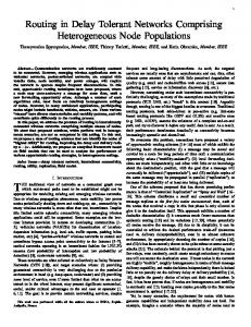
Figure 1: Message replica distribution through Binary Spray and Wait

1 3

3 1

1

1

2 1

3 4

1

5

2

1

2 1

1

4

4

2 3

2

1

6

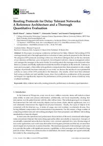
Figure 2: Message replica distribution through Fibonary Spray and Wait

When a node is left with only 1 copy, it switches to direct transmission. This trivial case can be summed up as a consequence of 1 being a Fibonacci number, so in accordance with clause 2 of our Fibonary Spray & Wait algorithm, direct transmission happens. Thus, our spraying algorithm in Fibonary Spray & Wait routing is actually determined alternately by the Fibonacci series, and Binary Spray & Wait algorithm. One distinct advantage of Fibonary Spray & Wait over Binary Spray & Wait is that, in Fibonary Spray & Wait, the direct transmission case is reached earlier than the corresponding Binary Spray & Wait Routing with the same number of copies. In other words, Fibonacci distribution is more asymmetric compared to the perfectly symmetric (half) division of message copies in Binary Spray & Wait. For example, let us consider the case of 10 copies with our starting node: Binary Spray & Wait divides 10 into 5 and 5, whereas our Fibonary algorithm divides it into 8 and 2 number of copies (see Figure 2). Now 8 may be further divided into 4 and 4 in subsequent iterations; but on the other hand 2 gets divided into 1 and 1, and hence direct transmission is reached in the 3rd level itself. For Binary Spray & Wait to reach direct transmission for initial number of copies as 10, it will need to go down to the 4th level in the spray-tree (Figure 1). However, the best case may be improved in Fibonary Spray & Wait, when we compare it with Binary for the same initial number of copies. This is actually a consequence of direct transmission being reached earlier, or in other words, the spray phase getting over earlier in one branch of the spray-tree. The Algorithm for the same is illustrated next. In the algorithm, ttlg = time to live of message g.

Algorithm 1: AtNodeA 1 2 3 4 5 6 7 8 9 10 11 12 13 14 15 16 17

for each message g with n copies at node A in the network do while ttlg > 0 do if a connection exists between current node A carrying message g and any other node B then if n is NOT a Fibonacci number then forward m copies of g to B keep n − m copies of g for itself if n is a Fibonacci number then forward ceil(n/2) copies of g to B keep floor(n/2) copies of g for itself if n = 1 then forward g to B iff B is the destination of g if g has not been received by node B earlier then accept g mark g as delivered delivered = delivered + 1 else discard g

IJECE Vol. 6, No. 6, December 2016: 3205 – 3216

IJECE

2.1.

ISSN: 2088-8708

3209

Mathematical Analysis

We assume that there are n nodes randomly distributed with a uniform distribution. Each message picks one of the remaining n − 1 nodes as its destination with an equal probability. For our algorithm, every message can have a maximum of ‘L0 copies but these ‘L0 copies are to be distributed among other nodes on the occurrence of a connection based on a predefined maxim. This maxim as already discussed earlier states that there are two possibilities for message distribution at every branching turn. The two cases that may arise are: 1. When ‘L0 is a fibonacci number: then tree distribution remains same as in Binary Spray & Wait. 2. When ‘L0 is not a fibonacci number: then suppose L = x such that, 0, 1, 1, 2, ...a, b, c...n is the fibonacci series where b < x < c. ∴ in integer series, the position of x with respect to fibonacci numbers a, b and c would be ...a, b, x, c... Now, in Binary Spray & Wait, this x would give rise to two divisions of ceil[n/2] and f loor[n/2]. In Fibonary Spray & Wait, it would be b and (x − b). To get a shorter branch we have to show that this difference (x − b) is less than x/2. Note that, b < x < c ....................(1) also, c − b = a ....................(2) Let x − b = d ....................(3) We have to prove that this difference (d) is always less than x/2. As ‘d0 is used in Fibonary Spray & Wait and x/2 is used in Binary Spray & Wait, the one with smaller value will give earlier wait phase. We know that d < a ....................(4) So if we can show a 6 x/2, d < x/2 can be deduced. Let us prove this using mathematical induction. ‘d’ has to be greater than 1 for x to be a non fibonacci number. ∴d>1 ⇒a>1 ∴ a is a minimum of 2, ∴ b is a minimum of 3, ∴ c is a minimum of 5, ∴ x is a minimum of 4, So the first possible value of x is 4. For x=4, 2 ⇒2

6 4/2 6 2 (true)

....................(5)

Let this be true for x = n, a 6 n/2 ....................(6) Now for x = (n + 1)/2, we have to show that, Fibonary Spray and Wait Routing in Delay Tolerant Networks (Priyanka Das)

3210

ISSN: 2088-8708

a 6 (n + 1)/2 We know, a

6 n/2

⇒a

6 n/2 + 1/2

⇒a

6 (n + 1)/2

....................(7)

Hence proved by mathematical induction. From (4), d < a, and a 6 (n + 1)/2 from (7) ∴ d < x/2. ∴ We are bound to get a branch in Fibonary Spray & Wait which renders quicker wait phase than the corresponding branch in Binary Spray & Wait. 3. RESULTS AND DISCUSSION 3.1. Simulation Setup We have done our simulation using the Opportunistic Network Environment (ONE) simulator (20), which is specifically designed for DTNs. A time step of 0.1s has been considered, i.e. any event recording is done after a time step of 0.1s. A new message is created every 25 to 35 seconds with message sizes varying between 500kB and 1M B. The simulation world size is 4500 × 3400meters. The movement model that we have chosen for all hosts in our simulation is the Shortest Path Map-Based Movement (SPMBM) model. The reason for this choice is that among the various movement models present this is the more realistic one wherein instead of a completely random walk, the nodes choose a random point on the map and then follow the shortest route to that point from their current location. Further details of the simulation parameters taken into consideration are discussed in Table 1. For fair comparison purposes we have compared our algorithm with different routing schemes in this genre namely the Spray & Wait (also called the Vanilla Spray & Wait) (8), Binary Spray & Wait (8) and Epidemic (3) (these schemes have already been discussed in Section II Previous Work). The results have been obtained after a rigorous simulation by varying the number of copies (L) over a period of 2 days. In addition, a comprehensive comparison of some of the popular existing routing protocols is shown in Table 2. The results are based on a simulation run for 24 hours in the ONE Simulator. The simulation parameters used are as discussed in Table 1. The initial number of messages L for Spray & Wait, Binary Spray & Wait and Fibonary Spray & Wait, has been taken as 12 for the simulations in Table 2. The graphs have been plotted using gnuplot. Table 1: Simulation Parameters Node Type Parameters Pedestrian Cars No. of Nodes 58 30 Speed 0.5 to 1.5 m/s 10 to 50 km/h Buffer Size 5 MB 5 MB Message Time To Live 300 minutes 300 minutes

3.2.

Trams 2 7 to 10 m/s 50 MB 300 minutes

Effect of Varying Number of Copies (L)

The number of copies(L) is by far the most important metric to be tested by variation for any variant of the Spray & Wait scheme (including our Fibonary). Hence we have compared the three variants of the Spray & Wait (Vanilla, Binary and Fibonary) by varying the value of L on a diverse range. A value of 7 for L has been considered as the lowest and 26 the highest. These simulations have been done on a constant time scale IJECE Vol. 6, No. 6, December 2016: 3205 – 3216

IJECE

ISSN: 2088-8708

3211

of 1 day i.e. 24hours. Since Epidemic Routing has no concept of maximum number of copies (L), we omit it in the comparison charts. Following is the detailed analysis of the effect of varying number of copies (L) on some selected performance parameters. 3.2.1.

Impact on Message Delivery probability

From the plot of Figure 3 it is prominent that for lower values of L, Fibonary Spray & Wait gives best message delivery probability among the considered schemes. For higher values of L, though not the best but Fibonary Spray & Wait shows consistent performance and is always better than Vanilla Spray & Wait (results say the message delivery probability of Vanilla Spray & Wait is on an average 3% less than that of Fibonary Spray & Wait). All in all it gives quite an impressive performance and good message delivery probability on all variations of L. 3.2.2.

Impact on Overhead Ratio

The overhead ratio is defined as the ratio of (Number of Messages Relayed - Number of Messages Delivered) to (Number of Messages Delivered). The overhead ratio of both Binary Spray & Wait and Fibonary Spray & Wait is understandably more than vanilla as they are more ambitious schemes, but out of the two the overhead of Fibonary Spray & Wait is less for lower values of L. Though it increases for higher values of L, it still gives a respectable performance. Hence this scheme works superfine for networks with lower values of L (usually small networks) and also for higher values of L as overhead is just a tad more than that of Binary Spray & Wait (see Figure 4). 3.2.3.

Impact on Message Latency

The average message latency for both Binary Spray & Wait and Fibonary Spray & Wait is more than Vanilla Spray & Wait on most occasions. From Figure 5, one can deduce that except when L = 7, average message latency in case of Fibonary Spray & Wait is much less than Binary Spray & Wait. On an average, the average message latency of Fibonary Spray & Wait is 1.2% less than that of Binary Spray & Wait. The results of message latency median though tell a different story. For lower values of L, Fibonary Spray & Wait works the best (see Figure 6) among all schemes considered. 3.2.4.

Impact on Message Hopcount

Message hopcount is the number of nodes that a message has to pass by before reaching its designated destination. Hence if hopcount can be kept to a bare minimum, one can cash on a number of things like saving buffer space, replica, route congestion etc. Simulation results show that though Vanilla Spray & Wait outperforms yet again, among the other two, Fibonary Spray & Wait performs better in most situations (see Figure 7 and Figure 8). Especially for L = 7, Fibonary Spray & Wait performs as good as Vanilla Spray & Wait (see Figure 8). 3.2.5.

Impact on Message Buffertime

The time a message spends on a buffer (source or intermediate) gives a clearer and more compact view of the delay incurred as well as the congestion created due to message replications. Thus this metric is of utmost importance and is one of the two most important things to be considered for every routing scheme in DTN (the other metric being message delivery probability). The plots of Figure 9 and Figure 10 show that in both cases of average message buffertime and buffertime median, Fibonary Spray & Wait performs way better than Vanilla Spray & Wait. In fact here the Vanilla Spray & Wait incurs huge delay, way above than the other two. Also Fibonary Spray & Wait performs better than Binary Spray & Wait. Speaking in numbers, on an average the average message buffertime of Fibonary Spray & Wait is 19% less than that of Vanilla Spray & Wait and 2.133% less than that of Binary Spray & Wait. Also the average message buffertime median of Fibonary Spray & Wait is 30% less than that of Vanilla Spray & Wait. So if we consider delay due to buffertime then our scheme works the best in the Spray & Wait genre. Fibonary Spray and Wait Routing in Delay Tolerant Networks (Priyanka Das)

3212

ISSN: 2088-8708

24

Binary SnW Vanilla SnW Fibonary

0.42

22

0.4

20 Overhead Ratio

Message Delivery Probability

0.44

0.38

0.36

16

14

0.32

12

10 5

10

15 20 No.of Copies (L)

25

30

Figure 3: Message Delivery probability (Simulation time for each is 24hours)

5

10

15 20 No.of Copies (L)

25

30

Figure 4: Overhead ratio (Simulation Time= 24hours)

3500

2800 Binary SnW Vanilla SnW Fibonary

2750

Message Latency Median(s)

3400 Average Message Latency(s)

18

0.34

0.3

Binary SnW Vanilla SnW Fibonary

3300

3200

Binary SnW Vanilla SnW Fibonary

2700 2650 2600 2550 2500

3100 2450 3000

2400 5

10

15 20 No.of Copies (L)

25

30

Figure 5: Average Message Latency (Simulation Time= 24hours)

5

10

15 20 No.of Copies (L)

3.5 Binary SnW Vanilla SnW Fibonary

Binary SnW Vanilla SnW Fibonary

3

3 Message Hopcount Median

Average Message Hopcount

30

Figure 6: Message Latency Median (Simulation Time= 24hours)

3.5

2.5

2

2.5

2

1.5

1.5 5

10

15 20 No.of Copies (L)

25

30

Figure 7: Average Message Hopcount (Simulation Time= 24hours)

5

10

15 20 No.of Copies (L)

25

30

Figure 8: Message Hopcount Median (Simulation Time= 24hours)

3200

2600 Binary SnW Vanilla SnW Fibonary

Binary SnW Vanilla SnW Fibonary

2400 Message Buffertime Median(s)

3000 Average Message Buffertime(s)

25

2800

2600

2400

2200

2000

1800

2200 1600 2000 5

10

15

20

25

30

No.of Copies (L)

Figure 9: Average Message Buffertime (Simulation Time= 24hours) 3.3.

10

15

20

25

30

No.of Copies (L)

Figure 10: Message Buffertime Median (Simulation Time= 24hours)

Effect of Varying Simulation Time

These simulation results show a candid performance which have been tested for short as well as long periods of time. For this effect we varied the time from 24hours (low) to 48hours (high). When varying the time quotient we have kept the number of copies (L) at a constant value of 26. This we do to show that even for IJECE Vol. 6, No. 6, December 2016: 3205 – 3216

IJECE

ISSN: 2088-8708

3213

high value of L, our scheme works just as fine as we have already seen how well it performs for lower values of L. 3.3.1.

Impact on Message Delivery probability

The bar graphs of Figure 11 depicts that Fibonary Spray & Wait has more message delivery probability than either Vanilla or Epidemic routing (Epidemic has on an average 43.1% lower delivery probability than Fibonary) over all periods of time tested. It though lags behind a little over Binary Spray & Wait but the difference is not much considering other metrics. 3.3.2.

Impact on Overhead Ratio

As expected, Figure 12 portrays that Vanilla Spray & Wait and Epidemic routing form the two opposite ends in the spectrum for overhead ratio. Our algorithm, Fibonary Spray & Wait is mezzo between the two techniques and gives a pretty impressive performance. In fact our scheme creates 97% lesser overhead as compared to Epidemic routing. 3.3.3.

Impact on Message Latency

The average message latency readings from the plot of Figure 13 shows that in terms of latency, Fibonary Spray & Wait performs better than Binary Spray & Wait (it incumbers averagely 1.232% lesser latency)and Epidemic routing (on an average 32.243% lesser) and compensates for its slightly lower message delivery probability than Binary Spray & Wait. Even if we consider the message latency median results, (see Figure 14), Fibonary Spray & Wait again shows better performance than Binary Spray & Wait and Epidemic routing (21.83% lesser) especially when running for longer stretches of time. 3.3.4.

Impact on Message Hopcount

The graphs of Figure 15 and Figure 16 shows a very interesting result, that at higher value of L(= 26), Binary and Fibonary Spray & Wait almost have the same average hopcount and along with Epidemic have similar hopcount medians for varied periods of simulation time. Furthermore, Fibonary Spray & Wait requires 24.4% lesser hopcounts than Epidemic routing. 3.3.5.

Impact on Message Buffertime

Figure 17 and Figure 18 again show that Fibonary Spray & Wait is a mezzo between the low buffertime of Epidemic and high buffertime of Vanilla Spray & Wait. Fibonary Spray & Wait performs quite decently with respect to both average as well as buffertime median giving 29.3% lesser message buffertime than Epidemic routing and 41.003% lesser buffertime median than Vanilla Spray & Wait. 3.4.

Extensive Comparison

Table 2 and Table 3 provide further comparison of Fibonary Spray & Wait with some more existing protocols. One can analyse from these tables how our proposed algorithm, Fibonary Spray & Wait, stands in comparison to the other established protocols present. We did not include the likes of MaxProp, PRoPHET etc in the previous detailed comparisons as they are part of a different category of protocols and are not affected by the parameters which affect Fibonary Spray & Wait ( like the variable L ). From Table 2 we observe that among the various routing protocols, the Fibonary Spray & Wait maintains a good balance between Delivery Probability, Overhead Ratio and Latency. In fact it comes second only to MaxProp in terms of Delivery Probability but beats it in all other metrics by a huge margin. Its Overhead Ratio is also on the lesser side and in Latency readings beats all other protocols but Spray & Wait. 4.

CONCLUSION In this work we have delved into the propitious routing problem of Delay Tolerant Networks. Though a considerable amount of research has been done in this field, there still is a huge scope for improvement as different kinds of DTNs can benefit from these schemes. Also optimal routing in DTNs being an NP hard Fibonary Spray and Wait Routing in Delay Tolerant Networks (Priyanka Das)

3214

ISSN: 2088-8708

Table 2: A Comparison Between Some Existing Routing Protocols and Fibonary Spray & Wait Simulation Results Routing Protocols Delivery Overhead Latency Latency Probability Ratio Average Median Epidemic Router 0.2491 42.2223 4509.5733 3404.1000 Spray & Wait Router 0.3461 14.0375 3143.7860 2579.0000 Binary Spray & Wait Router 0.3621 17.6189 3264.9631 2580.3000 Fibonary Spray & Wait Router 0.3703 17.1993 3220.5839 2580.3000 MaxProp Router 0.4305 23.0405 6942.4543 5952.8000 PRoPHET Router 0.2518 38.0258 4709.0958 3778.6000 First Contact Router 0.1896 34.7712 4944.5386 3801.8000 Direct Delivery Router 0.3184 0.0000 6549.6077 5725.0000

0.4 Binary SnW Vanilla SnW Fibonary Epidemic

40

0.35 35 Overhead Ratio

Message Delivery Probability

Binary SnW Vanilla SnW Fibonary Epidemic

0.3

0.25

30

25

20

15 0.2 24

36 Simulation Time(h)

48

Figure 11: Message Delivery probability (No. of Copies(L) = 26)

4200 4000 3800 3600

48

Binary SnW Vanilla SnW Fibonary Epidemic

3400

Message Latency Median(s)

4400

36 Simulation Time(h)

Figure 12: Overhead Ratio (No. of Copies(L) = 26)

Binary SnW Vanilla SnW Fibonary Epidemic

4600

Average Message Latency(s)

24

3200

3000

2800

3400 2600 3200 3000

2400 24

36

48

24

Simulation Time(h)

Figure 13: Average Message Latency (No. of Copies(L) = 26)

48

Figure 14: Message Latency Median (No. of Copies(L) = 26)

4

4 Binary SnW Vanilla SnW Fibonary Epidemic

Binary SnW Vanilla SnW Fibonary Epidemic

3.5 Message Hopcount Median

3.5 Average Message Hopcount

36 Simulation Time(h)

3

2.5

2

1.5

3

2.5

2

1.5

1

1 24

36

48

Simulation Time(h)

Figure 15: Average Message Hopcount (No. of Copies(L) = 26)

24

36

48

Simulation Time(h)

Figure 16: Message Hopcount Median (No. of Copies(L) = 26)

problem, one can only aim to work towards a particular specific goal. Hence we proposed our algorithm which works on the good points of the already established Binary Spray & Wait and yet improves on it by providing a IJECE Vol. 6, No. 6, December 2016: 3205 – 3216

IJECE

ISSN: 2088-8708

2800

2400 Binary SnW Vanilla SnW Fibonary Epidemic

Binary SnW Vanilla SnW Fibonary Epidemic

2200 Message Buffertime Median(s)

2600 Average Message Buffertime(s)

3215

2400

2200

2000

2000

1800

1600

1400 1800 1200 24

36 Simulation Time(h)

48

Figure 17: Average Message Buffertime (No. of Copies(L) = 26)

24

36 Simulation Time(h)

48

Figure 18: Message Buffertime Median (No. of Copies(L) = 26)

Table 3: Behavioural Characteristics of Some Popular DTN Routing Protocols and Fibonary Spray & Wait Routing Behavioural Characteristics Flooding Forwarding Utilisation of Upperbound on Upperbound on Protocols Family Family Network Knowledge Message Replica No. of Hops Epidemic X NO NO NO Router Spray & Wait X NO YES YES Router Binary Spray X NO YES YES & Wait Router Fibonary Spray X NO YES YES & Wait Router MaxProp YES (Based on X NO NO Router current connectivity) PRoPHET YES (Based on X NO NO Router past connectivity) First Contact X NO YES NO Router Direct Delivery X X NO YES YES Router

way to reach the wait phase earlier or later, giving it more choice and thereby improving its performance. Binary Spray & Wait is optimal on one assumption that all nodal movement is IID but in reality it is seldom possible so. Fibonary Spray & Wait betters on this aspect and gives the nodes more variety on the attainment of wait phase. This is proved mathematically as well as through extensive simulations on the ONE simulator. Through simulations one deduction is very clear that our scheme works best for smaller values of L and for longer stretches of time thus making it an excellent choice for recovery mechanisms in disaster struck areas where network is small due to maximum nodal failure and lower values of L is required due to energy constraints and also these protocols need to keep running for longer period of time unless SOS reaches the destination. REFERENCES [1] S. Burleigh, A. Hooke, L. Torgerson, K. Fall, V. Cerf, B. Durst, K. Scott, and H. Weiss, “Delay-tolerant networking: an approach to interplanetary Internet,” IEEE Communications Magazine, vol. 41, no. 6, pp. 128–136, 2003. [2] F. Warthman, “Delay-tolerant networks (dtns)- a tutorial,” 2003. [3] A. Vahdat and D. Becker, “Epidemic routing for partially connected ad hoc networks,” CS-200006, Duke University, Tech. Rep., 2000. [4] W. Ying, X. Hui-bin, and C. Dai-feng, “A novel routing protocol for vanets,” TELKOMNIKA Fibonary Spray and Wait Routing in Delay Tolerant Networks (Priyanka Das)

3216

ISSN: 2088-8708

Indonesian Journal of Electrical Engineering, vol. 11, no. 4, pp. 2195–2199, 2013. [Online]. Available: http://iaesjournal.com/online/index.php/TELKOMNIKA/article/view/2405 [5] K. Qureshi, A. H. Abdullah, A. Mirza, and R. W. Anwar, “Geographical forwarding methods in vehicular ad hoc networks,” International Journal of Electrical and Computer Engineering (IJECE), vol. 5, no. 6, 2015. [Online]. Available: http://iaesjournal.com/online/index.php/IJECE/article/view/7901 [6] P. Das, K. Dubey, and T. De, “Credit based routing in delay tolerant networks,” in Proc.of the 2nd IEEE International Conference on Parallel, Distributed and Grid Computing (PDGC). IEEE, 2012, pp. 158– 163. [7] P.Das, K.Dubey, and T.De, “Routing in delay tolerant networks using credit based spraying,” in Proc. 3rd IEEE International Advance Computing Conference (IACC). IEEE, 2013, pp. 218–223. [8] T. Spyropoulos, K. Psounis, and C. S. Raghavendra, “Spray and wait: an efficient routing scheme for intermittently connected mobile networks,” in Proc. SIGCOMM workshop on Delay-tolerant networking, ser. WDTN. ACM, 2005, pp. 252–259. [9] K. P. Thrasyvoulos Spyropoulos and C. S. Raghavendra, “Spray and focus: Efficient mobility-assisted routing for heterogeneous and correlated mobility,” in PerCom Workshops, 2007, pp. 79–85. [10] J. Burgess, B. Gallagher, D. Jensen, and B. N. Levine, “Maxprop: Routing for vehicle-based disruptiontolerant networks,” in Proc. IEEE INFOCOM, 2006. [11] A. Lindgren, A. Doria, E. Davies, and S. Grasic, “Probabilistic routing protocol for intermittently connected networks,” http://tools.ietf.org/html/draft-irtf-dtnrg-prophet-10, [Online; accessed 6-April-2013]. [12] U. Shevade, H. H. Song, L. Qiu, and Y. Zhang, “Incentive-aware routing in dtns,” in Proc. ICNP, 2008, pp. 238–247. [13] C. Liu and J. Wu, “An optimal probabilistic forwarding protocol in delay tolerant networks,” in Proc. 10th ACM, ser. MobiHoc. ACM, 2009, pp. 105–114. [14] E. P. Jones and P. A. Ward, “Routing strategies for delay-tolerant networks,” Submitted to ACM Computer Communication Review (CCR), 2006. [15] S. Jain, K. Fall, and R. Patra, “Routing in a delay tolerant network,” SIGCOMM Comput. Commun. Rev., vol. 34, no. 4, pp. 145–158, 2004. [16] K. P. T. Spyropoulos and C. S. Raghavendra, “single-copy routing in intermittently connected mobile networks,” in Proc. Sensor and Ad Hoc Communications and Networks SECON, 2004, p. 235244. [17] E. P. C. Jones, “Practical routing in delay-tolerant networks,” in Proc. WDTN. 237–243.

ACM Press, 2005, pp.

[18] E. Bulut, S. C. Geyik, and B. K. Szymanski, “Conditional shortest path routing in delay tolerant networks,” in Proc. WOWMOM, 2010, pp. 1–6. [19] Wikipedia, “Routing in delay-tolerant networking — wikipedia, the free encyclopedia,” http://en. wikipedia.org/w/index.php?title=Routing in delay-tolerant networking&oldid=593756339, 2014, [Online; accessed 8-April-2014]. [20] A. Ker¨anen, J. Ott, and T. K¨arkk¨ainen, “The one simulator for dtn protocol evaluation,” in Proc. of the 2Nd International Conference on Simulation Tools and Techniques, ser. Simutools ’09. ICST, 2009, pp. 55:1–55:10.

IJECE Vol. 6, No. 6, December 2016: 3205 – 3216