Automated Finite Element Computations in the FEniCS ... - KTH

Automated Finite Element Computations in the FEniCS Framework using General Purpose Graphics Processing Units On the road towards interactive simulation

FLORIAN

RATHGEBER

Master of Science Thesis Stockholm, Sweden 2010

Automated Finite Element Computations in the FEniCS Framework using General Purpose Graphics Processing Units On the road towards interactive simulation

FLORIAN

RATHGEBER

Master’s Thesis in Numerical Analysis (30 ECTS credits) at the Scientific Computing International Master Program Royal Institute of Technology year 2010 Supervisor at CSC was Johan Jansson Examiner was Michael Hanke TRITA-CSC-E 2010:106 ISRN-KTH/CSC/E--10/106--SE ISSN-1653-5715

Royal Institute of Technology School of Computer Science and Communication KTH CSC SE-100 44 Stockholm, Sweden URL: www.kth.se/csc

Abstract Graphics Processing Units (GPUs) are established as a computational hardware platform superior in price/performance compared to general CPUs, but typically require specialized implementations and expert low-level knowledge. In this thesis the FEniCS framework for automated finite element solution of partial differential equations is extended to automatically generate GPU implementations, and achieve the expected speedup without sacrificing generality. An implementation using NVIDIAs Compute Unified Device Architecture (CUDA) of general finite element assembly and a conjugate gradient (CG) solver for the linear system of equations are presented for the DOLFIN problem solving environment. Extending the FEniCS form compiler FFC to generate specific CUDA kernels for assembly from a mathematical notation of the variational form retains the flexibility and degree of automation which is the basis of FEniCS. A matrix-free method, computing the matrix-vector product Ax in the CG iteration without assembling the matrix A, is evaluated against the assembly method, and is shown to perform better for a class of problems. Benchmarking and profiling variational forms with different characteristics on a workstation show a significant speedup on the NVIDIA Tesla architecture of up to a factor 9 over the serial CPU implementation and reveal bottlenecks of both the CPU and GPU codes. Furthermore, a prototype implementation of computational steering for the FEniCS application Unicorn is presented, allowing to interactively change parameters of a running simulation and getting visual feedback in close to real time, presenting a possible application for GPU acceleration.

Referat Automatiserade finita-elementberäkningar i FEniCS-ramverket med hjälp av generella grafikkort (GGPU) - På väg mot interaktiv simulering Grafikkort (GPU) är etablerade beräkningsplattform överlägsen generella CPUer i avseendet pris/prestanda, men behöver typiskt specialiserade implementationer och lågnivåkunskap. I den här avhandlingen utökas FEniCS-ramverket för automatiserad finit-elementlösning av partiella differentialekvationer att automatiskt generera GPU-implementationerna och erhålla den väntade prestandaökningen utan att offra generalitet. En implementation som använder NVIDIAs Compute Unified Device Architecture (CUDA) av generell finit-elementassemeblering och en konjugerad gradient-lösare för det linjära systemet presenteras för DOLFIN-miljön för problemlösning. En utökning av FEniCS formkompilator FFC för att generera specifika CUDA-kärnor för assemblering från en matematisk notation av variationsformen behåller flexibiliteten och graden av automatiseringen som är grunden i FEniCS. En matrisfri metod som beräknar matris-vektorprodukten Ax i en CG-iteration utan att assemblera matrisen A jämförs mot en traditionell assembleringsmetod och visas att prestera bättre för en klass av problem. Benchmarks och profilering av variationala former med olika karakteristika på en arbetsstation visar en signifikant prestandaökning på en faktor 9 över en seriell CPU-implementation och visar flaskhalsar i både CPU och GPU-implementationerna. Vidare presenteras en prototypimplementation av beräkningsstyrning för FEniCS-applikationen Unicorn, som möjliggör interaktiv manipulation av parametrar i en aktiv simulering och visuell feedback i nära realtid, och visar en möjlig tillämpning av GPU-acceleration.

Acknowledgments

The work presented in this thesis came into being in great parts through a fruitful cooperation between the Computational Technology Laboratory (CTL) at KTH and the Software Performance Optimisation (SPO) Group at Imperial College London, established during the FEniCS’10 conference held in Stockholm in May 2010. Furthermore, this thesis owes its existence to the joint MSc program between FAU Erlangen and KTH Stockholm and its coordinators Dr. Michael Hanke and Dr. Lennart Edsberg in Stockholm and Prof. Dr. Ulrich Rüde and Dr. Harald Köstler in Erlangen. I would like to thank my supervisor Dr. Johan Jansson for giving me the opportunity to work on this topic, allowing me the freedom to shape it according to my interests, and many hours of discussion and constructive feedback. My special thanks go to Graham Markall, whom I owe a lot of inspiration for this work and who sustained a flood of emails and always had valuable advice. Furthermore I want to express my gratitude towards the SPO Group for providing me access to a machine with an NVIDIA Tesla C1060 card to do my computations on. Many practical hints and discussions about implementation aspects of DOLFIN and other parts of FEniCS with Niclas Jansson, Murtazo Nazarov, Cem Degirmenci, the whole CTL group and the helpful DOLFIN community, especially Dr. Garth N. Wells, Dr. Anders Logg, and Kristian B. Ølgaard, are gratefully acknowledged. My good friends and advisors in all things C++, Klaus Sembritzki and Thomas Heller, deserve my gratitude. And last but not least, I would like to thank my parents for their continuous support and always bringing me back to my senses when I got too ambitious, as well as my brother Martin for proofreading and fixing up my punctuation.

Contents

1 Introduction 1.1 Related Work . . . . . . . . . . . . . . . . . . . . . . . . . . . . . . . . . . .

1 2

I Background

3

2 The 2.1 2.2 2.3 2.4 2.5 2.6 2.7 2.8

Finite Element Method Variational Problems . . . . . . . . . Function Spaces . . . . . . . . . . . . Adaptivity . . . . . . . . . . . . . . . Assembly . . . . . . . . . . . . . . . Quadrature representation . . . . . . Tensor representation . . . . . . . . Solvers . . . . . . . . . . . . . . . . . Action of a Finite Element Operator

. . . . . . . .

. . . . . . . .

. . . . . . . .

. . . . . . . .

. . . . . . . .

. . . . . . . .

. . . . . . . .

. . . . . . . .

. . . . . . . .

. . . . . . . .

. . . . . . . .

. . . . . . . .

. . . . . . . .

. . . . . . . .

. . . . . . . .

. . . . . . . .

. . . . . . . .

. . . . . . . .

. . . . . . . .

. . . . . . . .

. . . . . . . .

. . . . . . . .

5 5 6 6 7 8 9 10 10

. . . .

. . . .

. . . .

. . . .

. . . .

. . . .

. . . .

. . . .

. . . .

. . . .

. . . .

. . . .

. . . .

. . . .

. . . .

. . . .

. . . .

. . . .

. . . .

. . . .

. . . .

. . . .

13 13 14 15 16

FEniCS Project FIAT . . . . . . . . . . . . . . . . . . . UFL, FFC, UFC . . . . . . . . . . . . DOLFIN . . . . . . . . . . . . . . . . . 4.3.1 Mesh . . . . . . . . . . . . . . . 4.3.2 Functions and Function Spaces 4.3.3 Assembly . . . . . . . . . . . . 4.3.4 Visualization and File I/O . . . Unicorn . . . . . . . . . . . . . . . . .

. . . . . . . .

. . . . . . . .

. . . . . . . .

. . . . . . . .

. . . . . . . .

. . . . . . . .

. . . . . . . .

. . . . . . . .

. . . . . . . .

. . . . . . . .

. . . . . . . .

. . . . . . . .

. . . . . . . .

. . . . . . . .

. . . . . . . .

. . . . . . . .

. . . . . . . .

. . . . . . . .

. . . . . . . .

. . . . . . . .

. . . . . . . .

19 19 19 20 20 22 22 23 23

3 Parallel Architectures 3.1 The NVIDIA Tesla Architecture 3.1.1 Concepts . . . . . . . . . 3.1.2 Programming Interface . . 3.2 Further Parallel Architectures . . 4 The 4.1 4.2 4.3

4.4

. . . .

. . . .

5 Computational Steering

25

II Design, Implementation and Results

27

6 DOLFIN for GPU 6.1 Finite Element Assembly on the GPU . . . . . . . . . . . . . . . . . . . . .

29 29

vi

. . . . . . . . . . . . . . . . .

29 30 32 32 34 34 35 35 36 36 37 38 39 39 40 44 46

7 Interactive Prototype 7.1 Design . . . . . . . . . . . . . . . . . . . . . . . . . . . . . . . . . . . . . . . 7.2 Implementation . . . . . . . . . . . . . . . . . . . . . . . . . . . . . . . . . . 7.3 Results . . . . . . . . . . . . . . . . . . . . . . . . . . . . . . . . . . . . . . .

47 47 48 50

IIIDiscussion

51

8 Conclusions and Future Work 8.1 Contributions . . . . . . . . . . . . . . . . . . . . . . . . . . . . . . . . . . . 8.2 Limitations . . . . . . . . . . . . . . . . . . . . . . . . . . . . . . . . . . . . 8.3 Future Work . . . . . . . . . . . . . . . . . . . . . . . . . . . . . . . . . . .

53 53 53 54

Bibliography

55

Appendices

61

A Hitchiker’s Guide to GPU Assembly

63

B UFL Files for Variational Forms

65

C Samples of Generated Code

67

6.2

6.3

6.4

6.1.1 The Assembly Loop Revisited . . . . . . . . . . . . . . 6.1.2 CUDA kernels for GPU Assembly . . . . . . . . . . . 6.1.3 A Question of Data Layout . . . . . . . . . . . . . . . 6.1.4 An Overview of DOLFIN GPU Classes . . . . . . . . Automating Assembly by Code Generation . . . . . . . . . . 6.2.1 FFC Compilation Workflow . . . . . . . . . . . . . . . 6.2.2 Generating Code for GPU Assembly . . . . . . . . . . 6.2.3 Integration of Generated Code with a User Program . Solving the Linear System . . . . . . . . . . . . . . . . . . . . 6.3.1 Conjugate Gradients for an Assembled Sparse Matrix 6.3.2 Conjugate Gradients Without Assembling a Matrix . 6.3.3 Comparing Computational Effort . . . . . . . . . . . . Profiling and Performance Results . . . . . . . . . . . . . . . 6.4.1 Profiling the Assembly . . . . . . . . . . . . . . . . . . 6.4.2 Assembly performance . . . . . . . . . . . . . . . . . . 6.4.3 Assembly-solve performance . . . . . . . . . . . . . . . 6.4.4 Interpreting Speedup Figures . . . . . . . . . . . . . .

. . . . . . . . . . . . . . . . .

. . . . . . . . . . . . . . . . .

. . . . . . . . . . . . . . . . .

. . . . . . . . . . . . . . . . .

. . . . . . . . . . . . . . . . .

. . . . . . . . . . . . . . . . .

. . . . . . . . . . . . . . . . .

Notation

The notation used in this thesis is adapted from Logg et al. (2011b) A AK A0 a aK A e FK GK I IK ιK K K0 L L LK L0 N nK ì `K i `0i PK P0 Pq (K) r uh U u Vˆ V Vˆh Vh φi φî φK i Φi T Ω

– – – – – – – – – – – – – – – – – – – – – – – – – – – – – – – – – – – – – – – –

the global tensor with entries {Ai }i∈I the element tensor with entries {AK i }i∈IK the reference tensor with entries {A0iα }i∈IK ,α∈A a multilinear form the local contribution to a multilinear form a from a cell K the set of secondary indices the error, e = uh − u the mapping from the reference cell K0 to K the geometry with entries {Gα K }α∈A Qρ tensor j the set j=1 [1, N ] of indices for the global tensor A Qρ the set j=1 [1, njK ] of indices for the element tensor AK (primary indices) the local-to-global mapping from [1, nK ] to [1, N ] a cell in the mesh T the reference cell a linear form (functional) on Vˆ or Vˆh the degrees of freedom (linear functionals) on Vh the degrees of freedom (linear functionals) on PK the degrees of freedom (linear functionals) on P0 the dimension of Vˆh and Vh the dimension of PK a degree of freedom (linear functional) on Vh a degree of freedom (linear functional) on PK a degree of freedom (linear functional) on P0 the local function space on a cell K the local function space on the reference cell K0 the space of polynomials of degree ≤ q on K the (weak) residual, r(v) = a(v, uh ) − L(v) or r(v) = F (uh ; v) the finite element solution, uh ∈ Vh PN the vector of degrees of freedom for uh = i=1 Ui φi the exact solution of a variational problem, u ∈ V the test space the trial space the discrete test space the discrete trial space a basis function in Vh a basis function in Vˆh a basis function in PK a basis function in P0 the mesh, T = {K} a bounded domain in Rd

Chapter 1

Introduction A world without numerical simulations is inconceivable for many scientists and engineers of today. Simulations have permeated the professional life of many people in these fields and are not only well established next to classical experiments but increasingly seek to replace them. Their success is largely due to the power of the mathematical methods they are based on, foremost the Finite Element Method (FEM) introduced in Chapter 2, and the rapidly increasing speed of computational hardware they are run on. The FEniCS project (Dupont et al., 2003, Jansson et al., 2010a) presented in Chapter 4 has set a milestone in the automated solution of differential equations with the FEM. It provides an abstract, high-level mathematical notation for the problem formulation, and a powerful interface in both Python and C++ to solve the problem and its underlying equations. Its core component is the library DOLFIN (Hoffman and Logg, 2002, Logg and Wells, 2010, Wells et al., 2009), providing a problem solving environment with mesh handling, assembly, solving, and output of the computed results. DOLFIN is complemented by a set of auxiliary components, a central part being the FEniCS Form Compiler FFC (Kirby and Logg, 2006, Wells and Logg, 2009). FFC translates the variational forms describing the problem into highly efficient C++ code used by DOLFIN to assemble the corresponding system of equations. Solving continuum mechanics equations is provided by the problem statement and solving environment Unicorn (Hoffman et al., 2011b, Jansson et al., 2010b). Today, simulations still largely follow the common workflow of setting up a problem, waiting for it to be solved, and only then be able to visualize the result, which is a major inconvenience. Running complex simulations on commodity hardware can be very timeconsuming. One often discovers that the input data or the problem setup needs to be modified or restated when analyzing the result, which equals updating the problem setup — if it is clear at all what needs to be changed — and starting all over again. In a sense, not only the answer is sought from the simulation, but many times also what question to ask. This is also true on supercomputers, where the batch queue systems and security designs preclude an interactive feedback loop. This thesis investigates two attempts to mitigate this inconvenience. Firstly, a prototype of computational steering, defined in Chapter 5, in the FEniCS framework is developed and evaluated in Chapter 7. This system provides the simulation user with a visualization of results as soon as they are computed, and control of the running simulation by interactively modifying a limited set of parameters, analogous to the interaction with a computer game (for an example of an interactive simulation system for “virtual claying” for prototyping CAD geometry, see Jansson and Vergeest, 2002). Secondly, the possibilities of accelerating finite element assembly and linear solve on contemporary commodity graphics hardware 1

CHAPTER 1. INTRODUCTION

are investigated in Chapter 6. To this end, DOLFIN is extended with data structures, an assembler, and solvers, all operating on a General Purpose Grahpics Processing Unit (GPGPU). The motivation and goal behind the second approach is the wish to run on the fastest and most appropriate hardware available to solve the problem at hand, without sacrificing the established and easy-to-use interface of FEniCS. GPU architectures introduced in Chapter 3 currently offer the highest computational capacity (in terms of floating point operations per second, flop/s) and the fastest memory access (in terms of memory bandwidth, GiB/s) per invested Dollar. Another goal of this work is to find the most suitable algorithms for solving a particular problem on a given hardware platform. Section 6.4.3 demonstrates that assembling the equation system as a global matrix and a subsequent solve is not the fastest in all cases.

1.1

Related Work

Parallelization of assembly for DOLFIN in combination with load balancing of adaptive mesh refinement has been successfully demonstrated by Jansson (2008), Jansson et al. (2010c) and has since led to the development of a High Performance Computing (HPC) branch of the DOLFIN library1 . GPUs were used for finite element computations already before they became easily programmable using GPGPU techniques, the first implementation of FEM on a GPU used texture hardware (Rumpf and Strzodka, 2001). Research mostly concentrated on solving the linear system of equations (Bell and Garland, 2008, 2009, Bolz et al., 2003, Krüger and Westermann, 2005). Klöckner et al. (2009) implemented a discontinuous Galerkin (DG) method on an NVIDIA GTX280, achieving speedups of 20 to 60 over a serial CPU implementation in single precision. DG methods are well suited to the GPU architecture, having a high ratio of largely independent computation to data transfer. Finite element assembly was brought on the GPU by Filipovic et al. (2009), investigating the granularity of assembly operations and their mapping to hardware threads as well as the benefits of performing all computations in a single monolithic kernel as opposed to splitting it into multiple kernels and storing intermediate results in global memory. Komatitsch et al. (2009) ported a high-order finite element earthquake model to CUDA, using mesh coloring to avoid data races when assembling the global matrix and hence achieving a speedup of 20 compared to their previous implementation in single precision. More recently, they extended their code using MPI to run on a large cluster of 192 GPUs (Komatitsch et al., 2010). A very systematic approach to finding the bottlenecks of FEM assembly on GPUs and evaluating a range of possible implementations was taken by Cecka et al. (2009). Markall et al. (2010) laid the foundation this work is based on, by combining finite element assembly on the GPU with a high-level description of the problem based on the domain-specific Unified Form Language UFL for the Fluidity finite element code (Gorman et al., 2009). Previous work of Markall (2009), Markall and Kelly (2009) demonstrated FE assembly for a Laplacian and an advection-diffusion example and solved the resulting equation system using a conjugate gradient linear solver on the GPU.

1 https://code.launchpad.net/~njansson/dolfin/hpc

2

Part I

Background

3

Chapter 2

The Finite Element Method This chapter presents the basic concepts of the finite element method (FEM), focusing on variational forms, assembly, adaptivity, tensor as well as quadrature representation of integrals, and matrix-free methods. It is based on Kirby and Logg (2011a,b,c), Ølgaard and Wells (2011), Logg (2007), Logg et al. (2011a), and the same notation is used. The introduction assumes the reader is familiar with the FEM, and is restricted to bilinear and linear forms. For a more comprehensive introduction, the reader is referred to mathematical textbooks such as (Brenner and Scott, 2008).

2.1

Variational Problems

Consider a general linear variational problem in the canonical form: Find u ∈ V such that ∀v ∈ Vˆ ,

a(v, u) = L(v)

(2.1)

where Vˆ is the test space and V is the trial space. The variational problem may be expressed in terms of a bilinear form a and linear form (functional) L, a : Vˆ × V → R, L : Vˆ → R. The variational problem is discretized by restricting a to a pair of discrete test and trial spaces: Find uh ∈ Vh ⊂ V such that a(vh , uh ) = L(vh )

∀vh ∈ Vˆh ⊂ Vˆ .

(2.2)

To solve the discrete variational problem (2.2), we make an ansatz of the form uh =

N X

Uj φj ,

(2.3)

j=1

ˆ and take vh,i = φî , i = 1, 2, . . . , N , where {φî }N i=1 is a basis for the discrete test space Vh N and {φj }j=1 is a basis for the discrete trial space Vh . It follows that N X

Uj a(φî , φj ) = L(φî ),

j=1

5

i = 1, 2, . . . , N.

CHAPTER 2. THE FINITE ELEMENT METHOD

We thus obtain the degrees of freedom U of the finite element solution uh by solving a linear system AU = b, where Aij = a(φî , φj ), bi = L(φî ).

i, j = 1, 2, . . . , N,

(2.4)

Here, A and b are the discrete operators corresponding to the bilinear and linear forms a and L for the given bases of the test and trial spaces. The discrete operator A is a — typically sparse — matrix of dimension N × N , whereas b is a dense vector of length N .

2.2

Function Spaces

The term finite element method stems from the idea of partitioning the domain of interest Ω of spatial dimension d into a finite set of disjoint cells T = {K}, K ⊂ Rd , typically of polygonal shape, such that ∪K∈T K = Ω. A finite element according to Brenner and Scott (2008), Ciarlet (1978) is a cell K paired with a finite dimensional local function space PK of dimension nK and a basis LK = K K 0 {`K 1 , `2 , . . . , `nK } for PK , the dual space of PK . nK The natural choice of basis for PK is the nodal basis {φK i }i=1 , satisfying K `K i (φj ) = δij ,

i, j = 1, 2, . . . , nK ,

(2.5)

which means it follows that any v ∈ PK may be expressed by v=

nK X

K `K i (v)φi .

(2.6)

i=1 nK The degrees of freedom of any function v in terms of the nodal basis {φK i }i=1 may be obtained by evaluating the linear functionals LK , which are therefore sometimes referred to as degrees of freedom of the resulting equation system. Defining a global function space Vh = span{φi }N i=1 on Ω from a given set {(K, PK , LK )}K∈T of finite elements requires for each cell K ∈ T a local-to-global mapping

ιK : [1, . . . , nK ] → [1, . . . , N ].

(2.7)

nK This mapping specifies how the local degrees of freedom LK = {`K i }i=1 are mapped to global N degrees of freedom L = {ì }i=1 , given by

`ιK (i) (v) = `K i (v|K ),

i = 1, 2, . . . , nK ,

(2.8)

for any v ∈ Vh , where v|K denotes the restriction of v to the element K.

2.3

Adaptivity

Estimates for the error e = uh − u in a computed finite element solution uh approximating the exact solution u of (2.1) relate the size of the error to the size of the (weak) residual 1 r : V → R defined by r(v) = a(v, uh ) − L(v). (2.9) 1 The

weak residual is formally related to the strong residual R ∈ V 0 by r(v) = (v, R).

6

2.4. ASSEMBLY

The error in the V -norm can be estimated as !1/2 kuh − ukV ≤ E ≡

C

X

2 ηK

.

(2.10)

K

with C a constant, K ∈ T the finite element discretization and ηK an error indicator on K. An adaptive algorithm to determine a mesh size h = h(x) such that E ≤ TOL successively refines an initial coarse mesh in those cells where the error indicator ηK is large. Possible strategies include refining the top fraction of cells where ηK is large, refining all cells where ηK is above a certain fraction of maxK∈T ηK , or refining a top fraction of all cells such that the sum of their error indicators account for a significant fraction of E. A new solution and new error indicators are computed on the refined mesh and the process repeated until either E ≤ TOL (the stopping criterion), a maximum number of refinement steps have been taken, or the available memory has been exhausted. The adaptive algorithm thus yields a sequence of successively refined meshes. For time-dependent problems, an adaptive algorithm needs to distribute both the mesh size and the time step size in the space-time plane. Ideally, the error estimate E is close to the actual error, as measured by the efficiency index E/kuh − ukV which should be close to one.

2.4

Assembly

The discrete operator A from (2.4) is usually computed by iterating over the cells of the mesh and adding the contribution from each local cell to the global matrix A, an algorithm known as assembly. If the bilinear form a is expressed as an integral over the domain Ω, we can decompose a into a sum of element bilinear forms aK , a=

X

aK ,

(2.11)

K∈T

and thus represent the global matrix A as a sum of element matrices, Ai =

X

AK i ,

(2.12)

[1, . . . , nj ] = {(1, 1), (1, 2), . . . , (n1 , n2 )}.

(2.13)

K∈T

where i ∈ IK , which is the index set IK =

2 Y j=1

These element or cell matrices AK are obtained from the discretization of the element bilinear forms aK on a local cell K of the mesh T = {K} K,1 K,2 AK i = aK (φi1 , φi2 ). n

(2.14)

j where {φK,j }i=1 is the local finite element basis for the discrete function space2 Vhj on K. i The cell matrix AK is a — typically dense — matrix of dimension n1 × n2 .

2 The

space Vh1 was earlier referred to as Vˆh and Vh2 as Vh .

7


Let ιjK : [1, nj ] → [1, Nj ] denote the local-to-global mapping introduced in (2.8) for each discrete function space Vhj , j = 1, 2, and define for each K ∈ T the collective local-to-global mapping ιK : IK → I by ιK (i) = (ι1K (i1 ), ι2K (i2 ))

(2.15)

∀i ∈ IK .

That is, ιK maps a tuple of local degrees of freedom to a tuple of global degrees of freedom. Furthermore, let Ti ⊂ T denote the subset of the mesh on which φ1i1 and φ2i2 are both nonzero. We note that ιK is invertible if K ∈ Ti . We may now compute the matrix A by summing local contributions from the cells of the mesh, X X aK (φ1i1 , φ2i2 ) Ai = aK (φ1i1 , φ2i2 ) = K∈Ti

K∈T

=

X K∈Ti

K,1 K,2 aK (φ(ι 1 )−1 (i ) , φ(ι2 )−1 (i ) ) 1 2 K K

=

X K∈Ti

AK . ι−1 (i)

(2.16)

K

This computation may be carried out efficiently by a single iteration over all cells K ∈ T . On each cell, the element matrix AK is computed and then added to the global matrix A as outlined in Algorithm 2.1. A=0 for K ∈ T (1) Compute ιK (2) Compute AK (3) Add AK to A according to ιK : for i ∈ IK + AιK (i) = AK i end for end for Algorithm 2.1: Assembly algorithm

2.5

Quadrature representation

A standard approach for evaluating the element matrix AK on the cell K of spatial dimension d (see Logg, 2007, Chapter 5.1) is known as quadrature. It refers to a summation of the basis functions and their derivatives as given by the variational form evaluated at a set of quadrature points and multiplied with suitable quadrature weights. Runtime execution of quadrature evaluation can be accelerated by using an affine mapping FK : K0 → K with pre-tabulated basis functions and derivatives at the quadrature points of the reference element K0 . The element matrix AK for Poisson’s equation is computed as Z K,2 K A = ∇φK,1 i1 · ∇φi2 dx K

≈

Nq X

(2.17) k wk ∇φK,1 i1 (x )

·

k=1

8

k 0 k ∇φK,2 i2 (x ) det FK (x ),

2.6. TENSOR REPRESENTATION N

N

q q with quadrature points {xi }i=1 ∈ K and corresponding quadrature weights {wi }i=1 scaled PNq such that i=1 wi = |K0 |. For polynomial basis functions, the quadrature points can be chosen such that the approximation (2.17) is exact. Assuming the two finite dimensional function spaces Vh1 and Vh2 the bilinear form a is

n1

n2

K,2 K K defined on are equal, the local basis functions {φK,1 i1 }i=1 and {φi2 }i=1 can be generated −1 k 0 as φK from the same basis {Φi }ni=1 i = Φi ◦ FK and the coordinates are given as x = k FK (X ). Hence the evaluation of the gradients of the basis functions is a matrix-vector product 0 −T ∇x φ K (xk )∇X Φi (Xk ) (2.18) i (xk ) = (FK )

for each quadrature point xk and each basis function φK i . Each gradient is computed in Nq · n0 · d2 multiply-add pairs and the total cost for the element matrix computation amounts to Nq · n0 · d2 + Nq · n20 · (d + 2) ∼ Nq · n20 · d, ignoring the cost of computing the mapping FK , its determinant, and the inverse of its Jacobian 0 FK . Note that this cost can be significantly reduced by applying optimizations such as loop invariant code motion, common subexpression elimination, and precomputation of constants as detailed in (Ølgaard and Wells, 2010).

2.6

Tensor representation

In many cases the evaluation of the element matrix AK can be accelerated by precomputing a reference tensor A0 on the reference element and contracting with a geometry tensor GK depending on the geometry of the current cell K (Kirby and Logg, 2006, 2007, Kirby et al., 2005a,b, Logg, 2007). We only consider the case where FK : K0 → K is an affine mapping and take the element matrix AK for Poisson’s equation as an exemple. Having AK i =

Z

K,2 ∇φK,1 i1 · ∇φi2 dx =

Z X d K β=1

K

∇

∂φK,1 ∂φK,2 i1 ∇ i2 dx ∂xβ ∂xβ n1

(2.19) n2

K,2 K K with spatial dimension d and local basis functions {φK,1 i1 }i=1 and {φi2 }i=1 , yields with a change of variables

AK i

Z X d d X d X ∂Xα2 ∂φ2i2 ∂Xα1 ∂φ1i1 0 × det FK dX, = ∂x ∂X ∂x ∂X β α β α 1 2 α =1 α =1 K0 β=1

0 and with det FK and the derivatives

0 AK i = det FK

∂X ∂x

constant due to the affine mapping FK

Z d d d d X d X X X X ∂φ1i1 ∂φ2i2 ∂Xα1 ∂Xα2 dX = A0iα Gα K, ∂x ∂x ∂X ∂X β β α α 1 2 α =1 α =1 α =1 α =1 1

2

(2.20)

2

1

β=1

1

K0

with A0iα

=

Z K0

∂φ1i1 ∂φ2i2 dX ∂Xα1 ∂Xα2

and 0 Gα K = det FK

d X ∂Xα1 ∂Xα2 . ∂xβ ∂xβ

β=1

9

(2.21)

2

(2.22)

(2.23)


The element matrix can hence be decomposed as AK = A0 : GK ,

(2.24)

with : the Frobenius product of matrices. A0 is the constant reference matrix that does not depend on the cell K and may be precomputed before the assembly of A, and GK the geometry matrix that needs to be computed for each cell K. The total computational cost for tabulating AK can be estimated as d3 + n20 d2 ∼ n20 d2 and compared to the cost Nq n20 d for quadrature. This results in a speedup of roughly Nq /d, which may be significant particularly for higher order elements.

2.7

Solvers

A finite element variational problem of the form (2.1) is translated through discretization and assembly to the linear system AU = b, (2.25) with A a generally sparse matrix, to be solved for the vector of unknowns U . This kind of linear system also appears in each iteration of a nonlinear scheme like Newton’s method. Efficient solvers include the family of Krylov-type iteration methods, such as the conjugate gradient (CG) iteration for symmetric positive-definite matrices (Hestenes and Stiefel, 1952), and the generalized minimal residual method (GMRES) (Saad and Schultz, 1986), which only require matrix-vector products, but not the matrix A in explicit form. Relaxation methods have been greatly superseded by multi-grid methods (Brandt, 1977), acting on a hierarchy of grids and solving in near linear time. More recently, direct solution methods based on Gaussian elimination have been successfully revived. The matrix A may not be particularly well-conditioned in the general case and hence the use of preconditioners can significantly improve convergence, especially for Krylov methods, whose convergence rate is directly related to the condition number of the matrix. A (leftsided) preconditioner transforms the linear system (2.25) into P −1 AU = P −1 b,

(2.26)

where P −1 is chosen to be a good approximation of A−1 , but at the same time cheap to compute 3 . Common choices for preconditioners given in Kirby and Logg (2011a) are classical relaxation methods, such as Gauss-Seidel, or incomplete factorizations, such as ILU (incomplete LU factorization). Multi-grid can also serve as a powerful preconditioner. For certain problem classes, there exist more advanced physically-based preconditioners, taking into account properties of the differential equations being solved.

2.8

Action of a Finite Element Operator

Krylov methods do not require the matrix A to be explicitly available, only the matrixvector product AW , which can be given as a “black box” in many implementations. Thus, they qualify for the use with so-called “matrix-free” methods and allow problems to be solved without ever explicitly computing or storing the matrix A. This section gives a brief overview of what is presented in Kirby et al. (2005a). 3 The inverse A−1 is the perfect preconditioner, resulting in a condition number of 1 for the preconditioned system, but requires solving the system.

10

2.8. ACTION OF A FINITE ELEMENT OPERATOR

Assembly of A is replaced by repeated assembly of a vector AW , the action of the operator A on the given vector W . We can express the vector w in terms of the nodal basis {φ2j }j∈I X w= Wj φ2j , (2.27) j∈I

where I is the set of global degrees of freedom. Now, for all i ∈ I X X X (AW )i = Aij Wj = a(φ1i , φ2j )Wj = a(φ1i , Wj φ2j ) = a(φ1i , w), j∈I

j∈I

(2.28)

j∈I

and v = AW is computed by evaluating a(φ1i , w) for all i ∈ I. Initially, all entries of v are set to zero and are then accumulated by looping over all elements K ∈ T with T the decomposition of the domain into elements, and computing +

vιK (i) =

|ιK | X

AK i,j wιK (j)

i = 1, . . . , |ιK |.

(2.29)

j=1

This can be written as a matrix-vector product for each element K +

vιK = AK wιK = (A0 : GK )wιK ,

(2.30)

where : is the Frobenius product of matrices, ιK denotes the set of global indices obtained from the local-to-global mapping of element K, A0 the reference tensor and GK the geometry tensor (see Section 2.6). The computational cost of (2.30) for Poisson’s equation is d2 |ιK |2 multiply-add pairs per element, with d the spatial dimension. An additional 3|ιK | + d(d + 1)/2 memory reads and writes are required, if the symmetry of GK is exploited, not counting storing AK . Note that v needs to be both read from and written to memory. The matrix-free approach has the disadvantage that preconditioners commonly used with Krylov methods usually involve manipulations of A and hence cannot be readily applied in this case. However, preconditioners can be adapted for the matrix-free approach if supported by the Krylov solver.

11

Chapter 3

Parallel Architectures Today, Moore’s Law (Moore, 1965, 1995) is not interpreted in terms of processor clock frequencies anymore1 , but rather in terms of processor core count. Multi- and many-core processors are a reality and pose challenges as well as provide opportunities for both hardware vendors and software developers. Graphics processing units (GPUs) received particular interest from the high performance computing (HPC) community with the advent of general purpose computations on theses cards, for which the term GPGPU was born (Thompson et al., 2002). This chapter introduces the latest NVIDIA GPU architectures (Lindholm et al., 2008), NVIDIA’s Compute Unified Device Architecture (CUDA) (NVIDIA, 2009a, 2010), and alternatives to NVIDIA both in hardware and software.

3.1

The NVIDIA Tesla Architecture

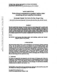
The central processing unit (CPU) is a multi-purpose processor, designed to deliver results with minimum delay by using sophisticated branch prediction, prefetching and a hierarchical cache, which are expensive in terms of transistor count and hence die size 2 (Akhter and Roberts, 2006). GPUs on the other hand are throughput oriented massively parallel coprocessors devoting a much higher percentage of their transistors to floating point ALUs3 , and thus are attractive for compute-intensive scientific applications. Figure 3.1 shows a simplified block diagram of a Tesla C1060 GPU with 240 streaming processor (SP) cores divided into 30 streaming multiprocessors (SMs), of which three each form an independent texture / processor cluster (TPC). Each SM contains eight SPs, one double-precision SP (DP-SP), two special functions units (SFU)4 , a multi-threaded instruction fetch and issue unit (MT), an instruction cache, read-only texture and constant caches, and 16 KiB of shared memory. An SP core is capable of delivering a scalar floating point multiply-add (MAD) and is clocked at 1.3 GHz. The single DP-SP per SM delivers a fused multiply-add (FMA) in double precision per clock cycle, and hence double precision comes with a performance penalty of 8 compared to single precision (NVIDIA, 2009b). The arithmetic peak performance of a Tesla C1060 is 933 GFlop/s 5 (billion floating point 1 Moore actually formulated his law in terms of integration density of integrated circuits. Stating it in terms of clock frequency is a common misconception. 2 Die refers to the actual silicon or a chip as exposed on the wafer. 3 ALU is the arithmetic logic unit. 4 The SFU is used for transcendental operations such as sin, cos, sqrt, exp, log. 5 Single precision Flop/s are calculated as 1.296 GHz clock * 30 SM * (8 SP per SM * 2 [one MAD per SP per cycle] + 2 SFU * 4 [four floating point units (FPU) per SFU with one flop per cycle]).

13

CHAPTER 3. PARALLEL ARCHITECTURES

0

1

SM

9 TCP

MT scheduler instr. cache const. cache

texture unit

texture unit

texture unit

interconnect network DRAM

DRAM

DRAM

DRAM

DRAM

DRAM

SP

SP

SP

SP

SP

SP

SP

SP

SFU

SFU

DP-SP shared mem

Figure 3.1: Block diagram of the NVIDIA Tesla GPU architecture with 30 streaming multiprocessors (SM), organized into 10 texture control processors (TCP), with eight streaming processors (SP) each

operations per second) in single precision and 78 GFlop/s 6 in double precision, provided all floating point computations are MADs. For coalesced reads from global memory, a bandwidth of up to 102.4 GB/s 7 can be reached for bursts8 .

3.1.1

Concepts

NVIDIA calls their processor architecture single-instruction, multiple-thread (SIMT)9 , since a group of 32 parallel threads called a warp execute the same instruction for each clock cycle. Each SM manages up to 24 warps, with a total of 768 threads. The SIMT instruction 6 Double precision Flop/s are calculated as 1.296 GHz clock * 30 SM * 1 DP-SP per SM * 2 [one FMA per cycle]. 7 The memory bandwidth is computed as 0.8 GHz memory clock * 2 (DDR memory) * 512 bit memory bus / 8 (since we want Byte). 8 See http://perspectives.mvdirona.com/2009/03/15/HeterogeneousComputingUsingGPGPUsNVidiaGT200. aspx for some background on how to compute these numbers. 9 SIMT was created in dependence on single-instruction, multiple-data (SIMD).

14

3.1. THE NVIDIA TESLA ARCHITECTURE

1 2 3 4 5 6 7

void saxpy (int n, float *c, float *a, float *b, float alpha ) { for (int i=0; i syntax. 11 A

15

CHAPTER 3. PARALLEL ARCHITECTURES

Designing parallel algorithms for GPUs more complex than the example above often requires a different approach and mindset as opposed to multi-threading on a CPU, which is more than one might expect from the syntactical similarities. For mere correctness of the algorithm one can safely ignore coalesced memory access, questions of data layout, and occupancy of the GPU’s streaming processors, but the result will perform poorly in most cases. Keeping the idiosyncrasies of the architecture in mind - some of which are discussed below - allows the avid programmer not only to write better performing, but often also more elegant code. • GPU kernels show a much more fine-grained level of parallelism, and threads are much more lightweight than one is used to from CPU threads. In graphics computations, one pixel is a common work unit for a thread, in numerical computations it could be one matrix or vector entry. • The GPU is an elephant, don’t feed it like an ant.14 That means GPUs are not suitable for low to moderate levels of parallelism. Several hundreds to thousands of threads15 are required to attain a good level of occupancy of the streaming processors, which in turn is essential for a good overall performance. • There is no automatically managed cache hierarchy16 , such that memory access means a load or store from or to DRAM and hence comes at a price (of several hundred clock cycles latency). Bandwidth is high compared to the CPU, provided memory access adheres to coalescing rules. Shared memory can help to achieve this17 , but must be explicitly instructed by the programmer to do so. • Barrier synchronization is only possible for threads on the same SM, there is no global synchronization mechanism. An implicit global synchronization only happens at kernel exit. Atomic operations are supported for integers only and are very costly, hence best to be avoided if that does not break correctness.

3.2

Further Parallel Architectures

CUDA is not the only way to harness GPUs for general purpose computations. AMD’s Radeon series of GPUs (former ATI) have similar architectural characteristics and compute capabilities18 . AMD’s counterpart to CUDA is the ATI Stream SDK (AMD, 2009), successor of the “Close to Metal” (CTM)19 technology. A common predecessor for both AMD Stream and CUDA was BrookGPU (Buck et al., 2004) developed at Stanford’s Graphics Lab. With the Open Compute Language (OpenCL) (mun, 2010), a vendor-independent parallel programming standard was created by Apple, which is now maintained by the Khronos Group, an industry consortium. It applies the stream programming paradigm to a range of multi-core platforms, not only to GPUs. Both AMD and NVIDIA actively support OpenCL through their SDKs. 14 http://forums.nvidia.com/index.php?s=&showtopic=98072&view=findpost&p=546413 15 Threads 16 Texture

need to be distributed to at least as many blocks as there are SMs, better twice as many. and constant cache are automatically managed but cannot always be used in scientific appli-

cations. 17 A common remedy for non-uniform (e.g. strided) memory access is to have all threads load data to shared memory in a coalesced fashion and read from there in the required pattern. 18 There are notable differences, which are out of scope of this work. 19 http://www.amd.com/us/press-releases/Pages/Press_Release_114147.aspx

16

3.2. FURTHER PARALLEL ARCHITECTURES

Another popular multi-core platform is the Cell Broadband Engine Architecture (often abbreviated Cell or Cell BE), developed by the STI alliance (Sony Computer Entertainment, IBM, and Toshiba) and well-known from its application as the processor of Sony’s PlayStation 3. It was specifically designed to deliver high performance for multimedia applications and consists of a Power Processing Element (PPE) and eight Synergistic Processing Elements (SPEs), linked together by an Element Interconnect Bus (EIB) (Gschwind, 2006). Intel’s advance into many-core visual computing is code-named Larrabee (Seiler et al., 2008) and consists of several in-order x86 CPU cores supplemented with a 512 bit SIMD vector processing unit, which is four times the SIMD width of current commodity CPUs. Larrabee is designed to be more efficient for processing parallel workloads than a traditional CPU while being more programmable and flexible than a modern GPU. A hybrid between these two worlds, it is capable of running an operating system through x86 compatibility, but also suited for graphics tasks by partly implementing a customizable rendering pipeline in hardware. At the time of writing, Intel was targeting the HPC market with Larrabee20 , but no product had been released yet. NVIDIA’s Fermi architecture is a further step towards convergence of CPU and GPU, with GPUs getting more general-purpose computing features. CPUs at the same time come with increased parallelism. At the time of writing Intel shipped the first 8-core Nehalem processor with up to 16 concurrent threads.

20 http://www.intel.com/pressroom/archive/releases/20100531comp.htm

17

Chapter 4

The FEniCS Project FEniCS (Dupont et al., 2003, Jansson et al., 2010a) is an open source software project founded in 2003 with the goal of automating Computational Mathematical Modeling (CMM). As outlined in Logg (2004), this involves automation of (i) discretization, (ii) discrete solution, (iii) error control, (iv) modeling, and (v) optimization. FEniCS was designed towards the three major goals generality, efficiency, and simplicity. Dynamic code generation is used to combine generality and efficiency, which are generally regarded as opposing goals. This chapter describes the most important components of FEniCS and how they interact to achieve the set goals. For a more comprehensive introduction, refer to Logg (2007).

4.1

FIAT

The FInite element Automatic Tabulator FIAT (Kirby, 2004, 2006, Rognes and Wells, 2009) is a Python library for the automatic tabulation of finite element basis functions over polynomial function spaces in one, two, and three space dimensions. FIAT generates quadrature points of arbitrary order on the reference simplex and tabulates the basis functions and their derivatives at any given set of points.

4.2

UFL, FFC, UFC

mathematical problem

weak form

form implementation

UFL

FFC

UFC interface

global matrix assembly

PDE solver

UFC

DOLFIN

Unicorn

Figure 4.1: UFL, FFC, and UFC as the link between the variational form in mathematical notation and the assembly in DOLFIN followed by solving in Unicorn (adapted from Alnaes et al., 2009) The FEniCS Form Compiler FFC (Kirby and Logg, 2006, Wells and Logg, 2009) automatically generates code for the efficient evaluation of element tensors from a given multilinear form specified in the Unified Form Language UFL (Ølgaard et al., 2009), a domainspecific language embedded in Python. FFC outputs optimized low-level code conforming to 19

CHAPTER 4. THE FENICS PROJECT

the Unified Form-assembly Code UFC (Alnaes et al., 2009) interface specification to a C++ header file. This file contains problem-specific code corresponding to the given multilinear form to be included in a user program or to be used with a UFC compliant FEM program, such as DOLFIN. The workflow from the mathematical notation to assembly code is shown in Figure 4.1. Alternatively, FFC can be called from a Python scripting environment to work as a just-in-time-compiler (JIT) for evaluation of multilinear forms. FFC supports element tensor evaluation by both quadrature and tensor contraction 1 (Kirby and Logg, 2007, Ølgaard and Wells, 2010, see also Sections 2.5 and 2.6), and internally calls FIAT for tabulation of the basis functions and quadrature points, if applicable. Optionally, an optimization of the form representation is available with the FErari (Finite Element ReARrangements of Integrals or Finite Element Rearrangement to Automatically Reduce Instructions) Python library (Kirby et al., 2005b, 2006, Kirby and Scott, 2007), significantly reducing the number of instructions required for element tensor evaluation.

4.3

DOLFIN

The core component of FEniCS is the Dynamic Object-oriented Library for FINite element computation DOLFIN (Hoffman and Logg, 2002, Logg and Wells, 2010, Wells et al., 2009), a UFC compliant C++ class library, augmented by a SWIG2 -generated Python interface. This allows for a seamless integration in a scripting environment with the remaining FEniCS components implemented in Python, and combines the performance of a C++ library with the versatility of a scripting language. Figure 4.2 illustrates the modular architecture of the DOLFIN library, with problemspecific input in form of the mesh, the variational form(s), and the finite element(s). The FFC form compiler translates the latter two into C++ code conforming to the UFC interface specification, and generates an additional thin layer wrapping UFC classes in corresponding DOLFIN classes and thus making them accessible. DOLFIN supports a range of different linear algebra backends out of the box, providing matrix and vector implementations as well as efficient linear solvers. At the time of writing, PETSc (Balay et al., 2010), Epetra (a part of Trilinos Heroux et al., 2005), MTL 4 (Gottschling et al., 2007), and uBLAS (Walter et al., 2009) were supported through thin wrappers. In the following, an overview of the central DOLFIN classes is given as shown in Figure 4.3, which represent the libraries’ key abstractions. As mentioned above, the linear algebra classes are essentially wrappers for external libraries, whereas the classes Form, FiniteElement, and DofMap wrap the FFC generated code. The DOLFIN developers decided against the use of templates, but use polymorphism where necessary, to allow for a less obfuscated and more readable code, and easier compilation and debugging. For a more comprehensive overview, see Logg and Wells (2010).

4.3.1

Mesh

A DOLFIN Mesh is a generic container for meshes of arbitrary topology in one to three space dimensions. The topology is defined through a set of mesh entities, tuples (d, i) with d the topological dimension and i a unique index of the entity within that dimension. Mesh entities represent vertices (topological dimension 0), edges(dimension 1), faces (dimesion 2), facets (co-dimension 1) and Cells (co-dimension 0)3 . The geometry is defined by a mapping 1 The

representation is chosen automatically based on efficieny considerations, but can be overridden. is the Simplified Wrapper and Interface Generator, http://www.swig.org. 3 A cell geometrically is an area in 2D, but a volume in 3D.

2 SWIG

20

4.3. DOLFIN

Figure 4.2: Modular DOLFIN library architecture (from Logg and Wells, 2010)

Figure 4.3: Central DOLFIN components and classes grouped by functionality (from Logg and Wells, 2010)

21


from vertices to space coordinates. Convenient access is provided by iterators. For details on storage and the automatic generation of topological information refer to Logg (2009).

4.3.2

Functions and Function Spaces

In accordance with the mathematical definition (see Section 2.2), a DOLFIN FunctionSpace is specified by a Mesh defining the domain, a FiniteElement defining the basis functions on a cell, and a DofMap defining the way local function spaces are pieced together on the domain. A Function is defined on a FunctionSpace, where multiple Functions can use the same FunctionSpace and hence automatically share Mesh, FiniteElement and DofMap. Coefficients are stored in a Vector, and Functions can be evaluated at arbitrary points, which equals an interpolation on the corresponding finite element. Arbitrary functions can be specified by subclassing Expression, basically a functor, and evaluated at arbitrary points. Both Function and Expression can be used as coefficients of a variational form. In addtion, the Constant class supplies constant coefficients.

4.3.3

Assembly

function assemble(a, A) A=0 for all K ∈ T do for j = 1, 2, . . . , r do Tabulate the local-to-global mapping ιjK end for for j = 1, 2, . . . , n do Extract the coefficient values wj on K end for Select cell integral 0 ≤ k ≤ nc such that K ∈ Tk Tabulate cell tensor AK for Ikc Add AK i to Aι1K (i1 ),ι2K (i2 ),...,ιrK (ir ) for i ∈ IK end for end function Algorithm 4.1: Assembly of the global tensor A corresponding to a bilinear form a from the local contributions on all cells (see Alnaes et al., 2009) DOLFIN provides a single assemble function for the assembly of arbitrary rank tensors (scalars, vectors, matrices, and higher order tensors) from multilinear forms. As given in Algorithm 4.1, the assemble function takes a Form of arity r with n coefficients as input and a GenericTensor of rank r as output parameter. For each cell of the mesh, the localto-global-mapping of degrees of freedom for each local function space as well as the values of all coefficients are tabulated. The latter are an input for tabulation of the element tensor, which is then added to the global tensor according to the degree of freedom mappings. This final step is illustrated in Figure 4.4 for a rank two tensor (a matrix). 22

4.4. UNICORN

Figure 4.4: Adding the element matrix AK to the global matrix A, where each entry is added to the row and column of A given by the local-to-global mappings ι1K and ι2K (from Alnaes et al., 2009)

4.3.4

Visualization and File I/O

To store computed results for visualization, DOLFIN provides XML output functions for most container classes such as Mesh, Matrix, and Vector using C++ operator overloading. Meshes in different formats4 can be read from file. Function data can be exported in the VTK XML format for visualization in VTKbased applications such as ParaView (Cedilnik et al., 2008). Built-in plotting functionality is available through Viper (Terrel et al., 2009).

4.4

Unicorn

Built on top of other FEniCS components, Unicorn (Hoffman et al., 2011a,b, Jansson et al., 2010b) automates simulations of continuum mechanics applications, providing a framework for fluid-structure interaction in turbulent incompressible and compressible flows on adaptive moving meshes. The mathematical basis is a unified continuum model consisting of canonical conservation equations for mass, momentum, energy, and phase on a continuum domain, and an adaptive stabilized FEM discretization on a moving mesh for tracking phase interface changes. Unicorn adds (i) duality-based adaptive error control, (ii) time-stepping non-linear solvers with adaptive fixed-point iteration, (iii) mesh adaptation through local refinement and coarsening (split, collapse, swap) as well as global cell quality optimization (smoothing), and (iv) slip / friction boundary conditions to the DOLFIN feature set. Interfaces to these components are combined in the Unicorn library, on top of which two primary solvers for incompressible fluid / solid with fluid-structure interaction, and compressible Euler (fluid only) are implemented. Key concepts are abstracted in classes of the Unicorn library as outlined by Hoffman et al. (2011b): Time-stepping TimeDependentPDE solves a non-linear system of type f (u) = −Dt u + g(u) = 0, 4 Gmsh,

Medit, Diffpack, ABAQUS, Exodus II, and StarCD are currently supported.

23

(4.1)


where g can include spatial derivatives, by fixed-point iteration in each time step. In weak form, the equation is (f (u), v) = (−Dt u + g(u), v) = 0

(4.2)

and the algebraic system F (U ) is solved by Newton-type fixed-point iteration (F 0 (UP ) · U1 , v) = (F 0 (UP ) · U1 − F (UP ), v)

(4.3)

with UP the previous iterate and F 0 = DU F (an approximation of) the Jacobian. Performance aspects of the implementation are discussed by Jansson (2009). Adaptive error control ErrorEstimate computes local error indicators that are the basis for the adaptive algorithm. The largest p% of the indicators are selected for refinement (see also Section 2.3). Space-time coefficient SpaceTimeFunction stores and evaluates a space-time function or coefficient needed for solving the dual problem. The dual solution at time s requires evaluating the primal solution U at time t = T − s. Friction boundary condition SlipBC models turbulent boundary layers by a friction model, where the normal condition u · n = 0, u ∈ Γ is “strongly” enforced in the algebraic system after assembly. This is necessary since turbulent boundary layers cannot be resolved with sufficient accuracy. Elastic mesh smoothing / optimization ElasticSmoother optimizes cell quality according to an elastic analogy for the whole mesh or parts of it. Mesh adaptation interface MeshAdaptInterface provides an interface to the MAdLib package (Compère and Remacle, 2009) enabling local mesh adaptation with operators such as edge split, edge collapse, and edge swap. These operators are used in the mesh adaptation control loop to satisfy a prescribed size h(x) and quality tolerance.

24

Chapter 5

Computational Steering Interactive control over a simulation process at runtime is referred to as computational steering (Gu et al., 1994, Mulder et al., 1998, Parker et al., 1997, van Liere et al., 1997) and is actively pursued as a field of research since the mid-1990s. Already in 1987, basic goals were formulated by the Visualization in Scientific Computing (ViSC) workshop (mcc, 1987): Scientists not only want to analyze data that results from super-computations; they also want to interpret what is happening to the data during super-computations. Researchers want to steer calculations in close-to-real-time; they want to be able to change parameters, resolution or representation, and see the effects. They want to drive the scientific discovery process; they want to interact with their data. The most common mode of visualization today at national supercomputer centers is batch. Batch processing defines a sequential process: compute, generate images and plots, and then record on paper, videotape or film. Interactive visual computing is a process whereby scientists communicate with data by manipulating its visual representation during processing. The more sophisticated process of navigation allows scientists to steer, or dynamically modify, computations while they are occurring. These processes are invaluable tools for scientific discovery. Immediate visual feedback can help researchers gain insight into scientific processes and anomalies, and can help them discover computational errors. [. . .] Almost 25 years after these findings, numerical simulation has not widely reached this vision yet, but still mostly consists of the steps identified by Parker et al. (1997): 1. Create or modify a discretized geometric model (computational mesh), 2. set up or modify initial and / or boundary conditions, 3. compute a numerical solution and store the result on disk, 4. visualize using a separate visualization package, 5. change the model according to the analysis, and 6. repeat the process from the beginning. 25

CHAPTER 5. COMPUTATIONAL STEERING

User

User Interface

Interpretation

Visualization

Manipulation

Communication and Data Transfer Data Collection

Application

Configuration

Reconfiguration Algorithm Adaption

Input Handling

Parameter Updating

Code Data and Parameters

Figure 5.1: Control flow diagram of a computational steering process (from Mulder et al., 1998)

Steps one and two are called pre-processing, step four post-processing. In a computational steering process as show in Figure 5.1, the distinction between preprocessing, post-processing and simulation is abolished. Instead, the user gets immediate visual feedback from the simulation since results are visualized as soon as they have been computed. After interpretation of the current result, the user can interactively change parameters as necessary and the changes are applied for the next time step or iteration of the running simulation. Times between changing parameters and viewing the result are greatly reduced compared to the traditional batch process, thereby allowing cause-effect relationships to become evident, that might otherwise have been overlooked. Computational steering closes the loop of problem specification, computation, and analysis, enhances productivity by shorter delays, and enables an experimental what-if analysis. Mulder et al. (1998) distinguish three main uses of computational steering in computational science and engineering: (i) model exploration for additional insight in the simulation by exploring parameter spaces, (ii) algorithm experimentation for switching between different implementations of e.g. linear solvers at runtime, and (iii) performance optimization trough e.g. interactive load-balancing of parallel applications. An overview of computational steering environments is given by Mulder et al. (1998), and Gu et al. (1994) present research in the field in an annotated bibliography.

26

Part II

Design, Implementation and Results

27

Chapter 6

DOLFIN for GPU Finite element methods on unstructured grids do not map particularly well to the GPU architecture through their irregular pattern of memory access and the low number of floating point computations per memory transfer. Cecka et al. (2009) identify the reduction step of adding the element matrix contributions to the global matrix as another potential performance bottleneck, since a high number of concurrently active threads trying to write to the same memory location lead to race conditions. These can be prevented either by an algorithm designed in a way that concurrent threads never write to the same memory location such as mesh coloring (Komatitsch et al., 2009), or by atomic writes to memory, leading to serialization of critical sections.

6.1 6.1.1

Finite Element Assembly on the GPU The Assembly Loop Revisited

Consider the assembly of a bilinear form with nw coefficients into a sparse matrix, where the local function spaces have a dimension of nd and the mesh consists of nc triangles and nv vertices. As detailed in Algorithm 4.1, the following data structures are needed: Local-to-global mapping of size nd for both function spaces and for each cell. Coefficient values for nw coefficients for each cell, where each coefficient has a local dimension given by its function space.1 Coordinates of size six (three vertices, two components per vertex) for each cell. Element tensor of size nd × nd for each cell. Global tensor of size nv × nv stored in a sparse format, where the number of non-zeros depends on the connectivity of the mesh. For parallel assembly, one CUDA thread per cell of the mesh2 is assigned. The loop over all cells is replaced by a single call to a corresponding CUDA kernel for each of the operations in the loop body of Algorithm 4.1, operating on all cells of the mesh at once and storing results in global memory. This results in Algorithm 6.1. 1 A single value per cell for a scalar discrete Galerking (P0) space, but 12 values for a second order (P2) vector space with two components on a triangle for instance. 2 Note that this is only one of several possible choices, a thread could be assigned to a global degree of freedom in the equation system (for a discussion of various options, see Cecka et al., 2009).

29

CHAPTER 6. DOLFIN FOR GPU

function assemble(a, A) dc = tabulate_dofs(1) dr = tabulate_dofs(2) for j = 1, 2, . . . , nw do wj = eval_coefficient(j) end for M = tabulate_tensor(w1 , . . . , wnw ) matrix_addto(A, M, dc , dr ) end function

. Tabulate local-to-global mapping ι1 . Tabulate local-to-global mapping ι2 . Extract coefficient values wj . Tabulate element matrices AK for all K . Add Ai to Aι1 (i1 ),ι2 (i2 ) for i ∈ I

Algorithm 6.1: Assembly of a bilinear form a into a sparse matrix A on the GPU, where each function is executed as a CUDA kernel for all cells K of the mesh at once. The localto-global mappings for the two function spaces a is defined for are denoted ι1 and ι2 , the set of indices of the block diagonal matrix of element matrices I.

6.1.2

CUDA kernels for GPU Assembly assembly time

assembly kernels

eval_expression tabulate_dofs

matrix_addto

tabulate_tensor interpolate_func

global memory

entity indices

referencing classes

GPUVector

function values

DOF mapping

GPUFunctionSpace

coefficient values

GPUMesh

GPUForm

vertex coords

element matrices

GPUAssembler

global matrix

GPUMatrix

Function

Figure 6.1: A data flow diagram showing input and output of the assembly kernels, how data is streamed between them, and where it is stored Figure 6.1 shows the interplay of the kernels involved in the assembly according to Algorithm 6.1, their inputs and outputs, and how they exchange data. tabulate_dofs takes entity indices from the mesh as input, and outputs the local-toglobal mapping for the corresponding function space, which determines the kind of mesh entities needed and the way they contribute to the mapping3 . evaluate_coefficients works differently depending on the type of coefficient (see Section 4.3.2), but in all cases outputs the coefficient values for all cells of the mesh. • Expressions or constant coefficients are either evaluated on the GPU directly if the expression is given as a CUDA kernel (eval_expression), or the expression evaluated on the CPU is transfered to the device. 3 Only cell indices are required for P0 elements, only vertex indices for P1 elements, vertices and edges for P2 elements.

30

6.1. FINITE ELEMENT ASSEMBLY ON THE GPU

kernel matrix_addto(v, M, dc , dr ) v=0 . Initialize the values to zero for i = 1, . . . , nr do . loop over the rows of the element matrix for j = 1, . . . , nc do . loop over the columns of the element matrix n = value_index(drthreadId,i , dcthreadId,j ) . get index into value array atomic_add(vn , MthreadId,i,j ) . atomically add entry to value array end for end for end kernel Algorithm 6.2: Atomically adds the element matrices M to the CSR value array v, where dr is the local-to-global mapping for the row space of M , dc that for the column space, and nr and nc denote the number of rows and columns of a single element matrix device function value_index(i, j) u = ri l = ri+1 while u > l do m = (u + l)/2 if cm < j then l =m+1 else u=m end if end while return l end device function

. get the lower bound for the index . get the upper bound for the index . do a bisection search . half the search interval . if the searched index is in the upper half. . . . . . . reset the lower bound . if the searched index is in the lower half. . . . . . . reset the upper bound . once the loop exits. . . . . . . the searched index is the lower bound

Algorithm 6.3: Finds the correct index into the CSR value array for matrix row i and column j by a bisection search on the column indices c, where r is the vector of row offsets

• Functions as coefficients are interpolated in GPU memory (interpolate_function) according to their associated function space. tabulate_tensor takes the vertex coordinates from the mesh and all coefficient values as input, and outputs the element matrices tabulated as given by the form. matrix_addto takes the element matrices as input, and adds them to the value array of the compressed sparse row (CSR) matrix (Shahnaz et al., 2005) according to the localto-global mappings, as outlined in Algorithms 6.2 and 6.3, based on Markall (2009). Note that the sparsity pattern of the matrix needs to be initialized for this to work. The CSR data structures are held in texture memory to benefit from caching, since memory access is not coalesced. The kernels tabulate_dofs and tabulate_tensor are generated by FFC from the form (see Section 6.2.2), whereas kernels to evaluate expressions are given by the user. Only the matrix_addto and interpolate_function kernels are implemented as part of the library. 31


6.1.3

A Question of Data Layout

The issue of where and how to store the data is crucial for GPU computations. All CUDA kernels involved in assembly work on all cells of the mesh in parallel and the data structures mentioned need to be allocated accordingly in global device memory before invocation, since no memory allocation is possible in a kernel.

thread ID

1 2 3

consecutive

thread ID

n-2 n-1 n

1 2 3

n-2 n-1 n

consecutive

Figure 6.2: GPU data layout to achieve coalesced transfers from and to global device memory (right) compared to a corresponding layout in CPU memory (left) Full bandwidth from global device memory can only be reached for coalesced memory transfer, and hence data layout should be designed such that threads read and write in the required consecutive pattern. Threads are associated with cells, hence data read or written in any single instruction needs to be stored consecutively in memory for consecutive cells. In other words, when regarded as a multi-dimensional array, the cell ID is the fastest running index. This is in contrast to the way data would be organized in CPU memory, where cells are processed consecutively and data is associated with each single cell stored consecutively in memory to maximize spatial locality of data access and hence cache performance. The difference in data layout is illustrated in Figure 6.2 and needs to be taken into account for all index computations. Note that the figure is for illustration only and does not reflect the actual DOLFIN CPU implementation, where data is only stored for the currently active cell at any given time. GPU computations typically require initial data to be transferred between host and device over the PCI-Express bus4 , and computed results to be transferred back from device to host, which should be kept to a minimum. Assembly requires entity indices and vertex coordinates from the mesh and coefficient values - if applicable - as initial data. Since the assembled matrix is used to solve the linear system on the device (see Section 6.3.1), only the final finite element solution needs to be transferred back to the host.

6.1.4

An Overview of DOLFIN GPU Classes

Figure 6.3 shows the classes collaborating to assemble a matrix on the GPU. 4 PCI-Express

16X delivers 4 GB/s per direction, compared to 102.4 GB/s on the device.

32

6.1. FINITE ELEMENT ASSEMBLY ON THE GPU

function

Expression fem

FunctionSpace GPUFunctionSpace local-to-global mapping

GPUExpression

Form

GPUConstant

GPUForm

GPUAssembler

coeff. values

element matrices

const. value mesh

linear algebra

Mesh

GenericMatrix GenericVector GPUMatrix

GPUMesh

row offsets col. indices matrix values

entity indices vertex coords

GPUVector vector values

Figure 6.3: Collaboration diagram of DOLFIN classes involved in GPU assembly with indication which data they store and which kernels they implement

GPUMesh holds vertex coordinates and entity indices and a reference to the Mesh for additional metadata. GPUFunctionSpace derives from FunctionSpace, holds the local-to-global mapping, and is subclassed by FFC-generated wrapper code implementing the tabulate_dofs kernel. GPUForm derives from Form, holds all coefficient values, and is subclassed by FFC-generated wrapper code. GPUMatrix represents a CSR matrix in device memory with row offsets, column indices, and the value array 5 . GPUVector represents a dense vector in device memory. GPUAssembler implements a static assemble function controlling the assembly process, and the matrix_addto kernel. GPUExpression derives from Expression and is subclassed to represent a function that can be evaluated at arbitrary points on the mesh used as a coefficient. This function is specified by the user as an eval_expression kernel for evaluation on the device. 5 GPUMatrix is actually an abstract base class implemented by a derived class of a suitable GPU backend. The same is true for GPUVector. This detail is omitted for simplicity.

33


GPUConstant derives from GPUExpression and is set to a constant scalar or vector value, representing a constant coefficient and implemented as an eval_expression kernel for evaluation on the device.

6.2

Automating Assembly by Code Generation

A crucial component for DOLFIN’s flexibility to handle diverse kinds of problems is the automated code generation by the FFC form compiler (see Section 4.2). To keep this advantage for GPU assembly, FFC was extended to automatically generate CUDA kernels for the tabulation of the local-to-global mapping and the element matrix. This section reviews FFC form compilation and briefly describes the necessary extensions and design decisions they are based on.

6.2.1

FFC Compilation Workflow

format

Poisson.ufl parser

Poisson.h

compiler FIAT

FERARI

Figure 6.4: Compilation of a variational form given as a UFL file to a UFC compliant header using FFC (adapted from Kirby and Logg, 2006). Parsing is entirely handled by UFL, the compilation relies on FIAT for tabulation of basis functions and FErari for optimization. Code is generated according to a format dictionary. Form compilation with FFC is a five-stage process, illustrated in Figure 6.4: (i) analysis, (ii) representation, (iii) optimization, (iv) code generation (with wrapper code generation as a substage), and (v) code formatting (Kirby and Logg, 2006). In the first stage, the parse tree generated by UFL from the .ufl form file is analyzed and metadata extracted, which is then passed to representation stage, choosing and generating either a tensor or quadrature representation with the help of FIAT. Optionally, this representation can then be passed to FErari for optimization before it is handed to the code generation stage for translation to C++ code using a format dictionary and predefined code snippets. If requested, wrapper code is added before proceeding to the final stage, where the generated function bodies are inserted into UFC compliant code templates and written either to a single header file or split into a header with definition and a cpp file with the implementation. 34

6.2. AUTOMATING ASSEMBLY BY CODE GENERATION

6.2.2

Generating Code for GPU Assembly

The first three FFC stages remain untouched; we only need to extend code generation and formatting to generate wrapper code for the DOLFIN GPU classes and the tabulate_dofs and tabulate_tensor kernels. Function bodies for the kernels differ from their UFC counterparts by indices into the data structures computed from the thread ID as described in Section 6.1.3, and a loop over all cells with a stride of the total number of threads6 . This only requires overriding a number of code snippets and entries in the format dictionary. UFC handles the variable number of coefficients of a form by passing a pointer-to-pointer to tabulate_tensor, thereby retaining a fixed function signature. Since this is not possible for a CUDA kernel7 , templates with function headers have to be adapted with an automatically generated argument list. Appendix C contains a comparison of generated CPU and GPU code for local-to-global mapping, and element matrix tabulation for Poisson on P2 triangle elements.

6.2.3

Integration of Generated Code with a User Program

Poisson.ufl

compile ffc -l dolfin-gpu

Poisson.ufl Poisson.h dolfin.h compile

Poisson.cu Poisson.h compile nvcc

ffc -l dolfin include

libdolfin.so

link

include

Poisson.o

main.cpp compile

dolfin-gpu.h

gcc

main.cpp link compile

user program

libdolfin-gpu.so

(a) using the DOLFIN library

gcc

user program

(b) using the DOLFIN-GPU library

Figure 6.5: Integration of generated code with a user program. FFC generated header files are meant to be included by .cpp files of user programs as shown in Figure 6.5a, but CUDA kernels can only be compiled by NVIDIA’s nvcc compiler 8 . 6 For

efficiency reasons, kernels are launched for a fixed number of blocks and threads per block. it is possible to pass a pointer to a region in device memory containing again pointers to device memory regions. This is fatal to performance however, since it means additional memory loads that cannot be coalesced. 8 The same is true for the implementation of the DOLFIN GPU classes in Section 6.1.4. 7 Technically

35


This means generated code needs to be split in a header containing the definitions, and a .cu file containing the kernels and calling code. Each kernel has an associated calling function that is also responsible for passing the right number of parameters for the kernel’s argument list. User programs need to link against the separately compiled CUDA code as shown in Figure 6.5b.

6.3 6.3.1

Solving the Linear System Conjugate Gradients for an Assembled Sparse Matrix

function preconditioned_conjugate_gradients(A, b, itmax , ε) i=0 x=0 r = b − Ax d = P −1 r . P −1 means application of the preconditioner δ0 = δnew = (r, d) while i < itmax & δnew > ε2 δ0 do q = Ad α = δnew /(dT q) x = x + αd r = r − αq s = P −1 r δold = δnew δnew = (r, s) q = δnew /δold d = s + βd i=i+1 end while end function Algorithm 6.4: The preconditioned conjugate gradient method for a symmetric positive definite matrix A and a preconditioner P (after Shewchuk, 1994) With the sparse matrix A and the right hand side vector f assembled9 , the linear system Au = f needs to be solved for u. Sparse linear systems are solved efficiently using the conjugate gradient method (Hestenes and Stiefel, 1952), given in Algorithm 6.4. This method is well suited for implementation on the GPU, only relying on the basic linear algebra operations spmv (sparse matrix-vector product), saxpy (vector addition and multiplication with a scalar), and scalar product. Implementation of the spmv based on Markall and Kelly (2009) is given in Algorithm 6.5, launched with one parallel thread per row to avoid data races and the CSR vectors held in texture memory to benefit from caching for non-coalesced memory access. The saxpy kernel is given in Algorithm 3.1, the scalar product is implemented as a parallel reduction (Nickolls et al., 2008) of the pairwise multiplied vector components. A Jacobi preconditioner was implemented to improve convergence (see Markall and Kelly, 2009, Chapter 5.2). 9 Vector

assembly was not specifically mentioned, but always implied, and similar considerations apply.

36

6.3. SOLVING THE LINEAR SYSTEM

kernel spmv(y, x, v, r, c) ythreadId = 0 for i = rthreadId , . . . , rthreadId+1 − 1 do + ythreadId = vi · x(ci ) end for end kernel Algorithm 6.5: Sparse matrix-vector multiplication of a vector x with a CSR matrix A given as the value array v, row offsets r, and column indices c, to produce a vector y.

6.3.2

Conjugate Gradients Without Assembling a Matrix

The conjugate gradient method at no point explicitly requires the matrix A, but only the matrix-vector-product v = Aw. Markall et al. (2010) hence suggest to avoid the assembly of A altogether, and instead compute v = Aw as the “action” of the operator A (Kirby et al., 2005a) according to Equation 2.30 for each cell K. That involves the three stages (i) scattering w according to the local-to-global mapping, (ii) multiplying each AK element matrix AK with the corresponding element vector wK as a dense matrix-vector operation in parallel for all K, and (iii) reducing the resulting vector again using the local-to-global mapping, to obtain v.

=

A

=

AT

Me

A

Figure 6.6: Linear algebra representation of the sparse matrix-vector multiplication without assembling the matrix, with M e the block-diagonal matrix of element matrices and A a sparse matrix representing the local-to-global mapping, where the rows represent all local and the columns the global degrees of freedom Alternatively, this can be written as (Markall et al., 2010) y = AT (M e (Av))

(6.1)

with M e the block-diagonal matrix of element matrices and A a sparse matrix representing the local-to-global mapping, shown in Figure 6.6. The rows of A represent all local and the columns the global degrees of freedom (DOF) with a single “1” entry per row at the column corresponding to the global DOF this local DOF is mapped to. The first two stages have been fused into a single kernel given in Algorithm 6.6. A global barrier is required before the third stage, which is implemented as an spmv similar to Algorithm 6.5, but optimized for the non-zeros of A all equal to one. For passing the necessary data structures to the solver, they are gathered in the class GPUKrylovSolver, holding the element matrices M , the local-to-global mapping d, as well 37


kernel stage12(t, v, M, d) for row r = 1, . . . , nr do tthreadId,r = 0 for column c = 1, . . . , nc do + tthreadId,r = MthreadId,r,c · v(dthreadId,c ) end for end for end kernel Algorithm 6.6: Stages one and two of the matrix-vector multiplication without assembly of A, corresponding to t = M e (Av) from (6.1). The element matrices are passed as M , the local-to-global mapping taking the role of A as d to produce the output vector t from input v. function inverse_mapping(r, c, d) c = sequence(1, |d|) c = sort_by_key(d) r = reduce_by_key(d,ones(|d|)) r = inclusive_scan(r) end function

. enumerate local DOFs . sort enumerated DOFs by mapping as key . get non-zeros per row by reduction . get final row offsets by prefix scan

Algorithm 6.7: Computes the column indices c and row offsets r for the “inverse” degreeof-freedom mapping needed for the spmv in the third stage of applying the operator A to a vector. All computation is done on the device by efficient kernels of the thrust parallel algorithms library (Hoberock and Bell, 2010).

as the column indices c and row offsets r needed for the spmv. Note that these are not the same as those in the CSR representation of A, but represent an “inverse” of the local-toglobal mapping, where its contributing element matrix entries are assigned to each global degree of freedom. Algorithm 6.7 shows computation of c and r. A Jacobi preconditioner is implemented by assembling the diagonal of A to a vector, which is efficiently done by applying an spmv as in stage three described above to the vector of diagonals of all element matrices, and taking the reciprocal of each component. However, avoiding the assembly of the right hand side is not possible, since it is explicitly required by the solver. Markall et al. (2010) propose a way to avoid atomic operations for the reduction of element vectors to the right hand side vector f = AT f e by applying the same spmv kernel as shown above in stage three10 .

6.3.3

Comparing Computational Effort

Markall et al. (2010) note that the matrix-free method implies additional cost for the sparse matrix vector product in the solver in terms of floating point computations and memory transfer compared to the assembled matrix. This additional cost is proportional to the average number of elements incident to each node of the mesh, referred to as the variance of the mesh, and needs to be evaluated against the benefit of saving costly atomic operations 10 This does not map to the classes as they are implemented in DOLFIN. The vector assembly has no access to the column indices and row offsets needed for the spmv. Those have to be recomputed since they are stored in GPUKrylovMatrix.

38

6.4. PROFILING AND PERFORMANCE RESULTS

in the addto algorithm, and initialization of the matrix with the sparsity pattern. Since the addto needs to be done only once per assembly but the spmv for each iteration of the Krylov iteration, we can assume this trade-off depends on the number of time steps solved per assembly of the matrix and the number of iterations required to converge for each time step. Incrementing either of both numbers equals a smaller share of total time for assembly as compared to solve, which can be expected to increasingly favor the assembly approach.

6.4

Profiling and Performance Results

All benchmarks were performed on a system with Intel Core2 Duo E8400 CPU running at 3.00 GHz, 2 GiB of RAM and an NVIDIA Tesla C1060 GPU running at 1.30 GHz core clock with 4 GiB of GDDR memory running at 800 MHz. Details on the device can be found in 3.1. C++ code was compiled using gcc 4.2.4 with the O3 option, CUDA code using nvcc 3.0. The following versions of the FEniCS libraries were used: DOLFIN 0.9.8, FFC 0.9.3, FIAT 0.9.2, UFC 1.4.1, and UFL 0.5.3.

Figure 6.7: Discretization of the unit square by a uniform triangle grid All forms were compiled with FFC using tensor representation and optimization disabled. Benchmarks comparing optimized and non-optimized tensor contraction revealed insignificant differences in performance and the CUDA compiler occasionally had difficulties compiling the optimized code. Comparing quadrature against tensor representation showed a performance advantage for the tensor representation. All computation was done in double precision. The problems were discretized on a uniform triangle grid on the unit square as shown in Figure 6.7.

6.4.1

Profiling the Assembly

To determine the performance bottleneck, profiling results for GPU assembly of two forms with different characteristics are presented in this section. The first being Poisson’s equation on a triangle mesh with piecewise constant (P1) basis functions without coefficients, given 39


as a=

Z

∇u · ∇v dx,

(6.2)

the second being the momentum term from the stabilized Navier-Stokes equations on a triangle mesh, given as Z a = v · u + 0.5 k (ν(∇v · ∇u) + ∇v · (w · ∇u) dx Z (6.3) + 0.5 k (d1 ((w · ∇v) · (w · ∇u)) + d2 (∇ · v)(∇ · u)) dx, with the scalar coefficients k, ν, d1 , d2 , and the vector coefficient w. The profiles in Figure 6.8 compare the relative amount of GPU execution time spent in each kernel for assembling the global CUDAMatrix (orange) and initializing the GPUKrylovMatrix for the matrix-free method (blue). For both forms between 70 and 80% of GPU execution time is spent in the addto for assembly, whereas for matrix-free 70 to 80% are spent in thrust kernels and block_gather 11 . Copying initial data from host to device (memcpyHtoD) accounts for 8 to 23%, whereas tabulation of the element matrices only takes about 4% for Poisson and about 10% of the total time for stabilized Navier-Stokes. The computation of coefficients for Navier-Stokes in GPUSource and GPUVelSource is almost negligible with less than 2%.

6.4.2

Assembly performance

Form Poisson 1st order Poisson 2nd order Poisson 3rd order Navier-Stokes

elem. mat. 3×3 6×6 10 × 10 6×6

coefficients 0 0 0 4 scalar, 1 vector

# operations for elem. mat. comp. 30 (CPU) / 43 (GPU) 68 (CPU) / 108 (GPU) 224 (CPU) / 328 (GPU) 351 (CPU) / 511 (GPU)

Table 6.1: Overview of cost for computing element matrices of the forms used (the higher operation count on the GPU is due to index calculations) The DOLFIN Assembler with PETSc backend is evaluated against GPUAssembler for Poisson’s equation without coefficients on elements of degree one to three, and the momentum term from the stabilized Navier-Stokes equations with coefficients as described above, both on a triangle mesh. Characteristic properties of the forms are given in Table 6.1. Performance in terms of assembled cells per second is given in Figure 6.9 for assembly (a) and reassembly (b). The forms widely differ in cost due to the different sizes of the element matrices given in Table 6.1, with the third order Poisson the most, the first order Poisson the least expensive, and the stabilized Navier-Stokes in between orders two and three. Initializing the matrix is comparable to the assembly in computational cost, which explains the performance gain of about a factor five in reassembly, where matrix initialization is not measured. Figure 6.10 shows the speedup of the GPU implementation over the DOLFIN reference implementation using the PETSc backend for assembly (a) and reassembly (b). The high cost of matrix initialization is evident once more from the graphs, with speedups dropping from a level of three to nine in (b) to 2.5 or less in (a). The speedup is particularly good 11 These

are required for building the inverse local-to-global mapping, see Section 6.3.2.

40


GPU kernel execution time (%) 0

10

20

30

40

50

60

70

80

90

tabulate_dofs tabulate_tensor matrix_addto block_gather thrust memcpy memcpyHtoD memcpyDtoH

(a) Poisson’s equation on first order triangles

GPU kernel execution time (%) 0

10

20

30

40

50

60

70

80

tabulate_dofs GPUVelSource GPUSource tabulate_tensor matrix_addto block_gather thrust memcpy memcpyHtoD memcpyDtoH

(b) Stabilized Navier-Stokes momentum term on first order triangles

Figure 6.8: Relative GPU execution time spent in each kernel for matrix assembly (orange), 41 and maxtrix-free (blue)


Assembled cells/s

1e+07

CUDA, NSE momentum (coefficients) CUDA, Poisson 3rd order CUDA, Poisson 2nd order CUDA, Poisson 1st order PETSc, NSE momentum (coefficients) PETSc, Poisson 3rd order PETSc, Poisson 2nd order PETSc, Poisson 1st order

1e+06

100000 32768

73728

131072

294912

524288

1.17965e+06

294912

524288

1.17965e+06

Number of cells

(a) Assembly 1e+08

CUDA, NSE momentum (coefficients) CUDA, Poisson 3rd order CUDA, Poisson 2nd order CUDA, Poisson 1st order PETSc, NSE momentum (coefficients) PETSc, Poisson 3rd order PETSc, Poisson 2nd order PETSc, Poisson 1st order

Assembled cells/s

1e+07

1e+06

100000 32768

73728

131072 Number of cells

(b) Reassembly

Figure 6.9: Assembly performance measured in assembled cells per second

42


2.4

CUDA, NSE momentum (coefficients) CUDA, Poisson 3rd order CUDA, Poisson 2nd order CUDA, Poisson 1st order

2.2

Speedup

2

1.8

1.6

1.4

1.2 32768

73728

131072

294912

524288

1.17965e+06

294912

524288

1.17965e+06

Number of cells

(a) Assembly 10

9

CUDA, NSE momentum (coefficients) CUDA, Poisson 3rd order CUDA, Poisson 2nd order CUDA, Poisson 1st order

8

Speedup

7

6

5

4

3

2 32768

73728

131072 Number of cells

(b) Reassembly

Figure 6.10: Speedup of GPU assembly over PETSc

43


for the Navier-Stokes form, which has many coefficients that can be efficiently evaluated on the GPU. Lower order Poisson performs better on the GPU due to the relatively greater share of element matrix tabulation compared to addto.

6.4.3

Assembly-solve performance 64

Poisson 3rd order, CUDA LMA Poisson 3rd order, CUDA assemble Poisson 3rd order, PETSc LMA Poisson 3rd order, PETSc assemble Poisson 1st order, CUDA LMA Poisson 1st order, CUDA assemble Poisson 1st order, PETSc LMA Poisson 1st order, PETSc assemble

32

16

Runtime [s]

8

4

2

1

0.5

0.25 2

4

8

16 Number of iterations

32

64

128

Figure 6.11: Total times for assembly and solve Runtimes for assembling the global matrix and right hand side vector from 524288 elements and solving for a number of iterations are shown in Figure 6.11, where “assemble” denotes the assembly and “LMA” denotes the matrix-free method (local matrix approach). They are of the form t = α · nit + β, with α the time to compute a single iteration, β the startup time (including assembly where applicable), and nit the number of iterations performed by the solver. For better visualization of break-even between assembly and matrix-free method, the curves are plotted with logarithmic axes and hence are not linear. The matrix-free method is beneficial for low iteration numbers since addto and matrix initialization is saved for the price of a more expensive matrix-vector product in the solve. Break-even points with the assembly method in total runtime for PETSc and CUDA backends can be found at 16 and 60 iterations respectively for first and at 25 and beyond 1000 iterations - if it breaks even at all - respectively for fourth order Poisson. The penalty for the addto significantly increases with increasing order, and becomes prohibitive so that particularly high-order element benefit from the matrix-free method. Speedups of the GPU implementation over the DOLFIN reference for the whole assembly and solve are in the range of 1.5 to three, slightly higher for the solve only. The matrix-free 44

6.4. PROFILING AND PERFORMANCE RESULTS 4

Poisson 3rd order, CUDA LMA Poisson 3rd order, CUDA assemble Poisson 3rd order, PETSc LMA Poisson 1st order, CUDA LMA Poisson 1st order, CUDA assemble Poisson 1st order, PETSc LMA

3.5

Speedup (factor)

3

2.5

2

1.5

1

0.5 2

4

8


32

64

128

32

64

128

(a) Assembly and solve 4

Poisson 3rd order, CUDA LMA Poisson 3rd order, CUDA assemble Poisson 3rd order, PETSc LMA Poisson 1st order, CUDA LMA Poisson 1st order, CUDA assemble Poisson 1st order, PETSc LMA

3.5

Speedup (factor)

3

2.5

2

1.5

1

0.5

0 2

4

8


(b) Solve only

Figure 6.12: Speedup of GPU implementation over DOLFIN reference implementation with PETSc backend 45


method in PETSc is a custom implementation12 very close to the GPU implementation, and has a performance disadvantage independent of the number of iterations.

6.4.4

Interpreting Speedup Figures

Comparing the obtained speedup figures to common results in GPU computing, a number of comments are in order. • All computations presented in the previous sections are performed in double precision, resulting in a penalty of factor eight for floating point computation and factor two for memory transfer on the Tesla architecture, as noted in Section 3.1. With 78 GFlop/s peak performance in double precision, the NVIDIA Tesla C1060 Is about on par with a current Intel Nehalem 8-core CPU. The new Fermi architecture brings down the double precision penalty to only two, introduces a two-level cache hierarchy, and significantly improves peak performance, so that considerably higher speedups can be expected from future GPU architectures. • High speedup numbers are often due to comparisons of mediocre CPU implementations with highly optimized GPU implementations (Lee et al., 2010). With the implementation presented in this chapter, it is almost the other way round. A highly optimized linear algebra (PETSc) and tensor contraction (generated by FFC) implementation is compared against generated GPU kernels without any hand-optimization and a textbook implementation of the conjugate gradient method in CUDA. Tuning the code generation and optimizing the linear solver leave some scope for further performance improvement. • Performance comparisons between CPU and GPU often neglect data transfer between host and device or even try to eliminate delays such as kernel startup times from speedup calculations. The performance numbers presented in this chapter are true one-to-one comparisons including all transfer and setup times.

12 The matrix-free method was implemented using the PETSc library calls MatCreateShell and MatSetShellOperation.

46

Chapter 7

Interactive Prototype Feasibility of interactive simulations in the FEniCS framework is demonstrated in this chapter by a prototype implementation of a computational steering environment using Unicorn.

7.1

Design

FEniCS implements the complete simulation process including the problem statement with initial and / or boundary conditions, but relies on external tools for pre-processing (geometry / mesh generation) and post-processing (visualization). To close the interactive feedback loop described in Chapter 5, the Unicorn solvers need to provide an interface for accepting parameter changes and a way to update the visualization once computation of a time step finishes.

visualization

client

server start simulation

initialization

time stepping read file

init GUI

change params

initial parameters

param changes

network

update

timestep finished

finalization

simulation finished

update params

solve

t