Finite Element Computations of KPP Front Speeds

Finite Element Computations of KPP Front Speeds in Random Shear Flows in Cylinders ∗ Lihua Shen†, Jack Xin‡, and Aihui Zhou§

Abstract We study the Kolmogorov-Petrovsky-Piskunov (KPP) minimal front speeds in spatially random shear flows in cylinders of various cross sections based on variational principle and an associated elliptic eigenvalue problem. We compare a standard finite element method and a two-scale finite element method in random front speed computations. The two-scale method iterates solutions between coarse and fine meshes, and reduces the cost of the eigenvalue computation to that of a boundary value problem while maintaining the accuracy. The two-scale method saves computing time and provides accurate enough solutions. In case of square and elliptical cross sections, our simulation shows that larger aspect ratios of domain cross sections increase the average front speeds in agreement with an asymptotic theory.

Key words: KPP front speeds, random shear flows in cylinders, stochastic eigenvalue problems, two-scale finite element method. AMS subject classifications: 65C30, 65C05, 65N30, 65N25.

∗ This work was partially supported by the National Science Foundation (NSF) of China under grant 10425105, the National Basic Research Program under grant 2005CB321704, and US NSF Grant DMS-0549215. † Department of Mathematics, Capital Normal University, Beijing 100037, China ‡ Department of Mathematics, University of California at Irvine, Irvine, CA 92697, USA § LSEC, Institute of Computational Mathematics and Scientific/Engineering Computing, Academy of Mathematics and Systems Science, Chinese Academy of Sciences, P.O.Box 2719, Beijing 100080, China

1

1

Introduction

Front propagation in heterogeneous flows is an active research area in applied science and mathematics [7, 14, 15, 18, 19, 25, 32, 33, 36]. A fundamental problem is to characterize and compute large scale front speeds in random flows [10, 19, 30, 31, 39]. The Kolmogorov-Petrovsky-Piskunov (KPP) minimal front speeds admit a variational characterization in terms of principal eigenvalue or principal Lyapunov exponent of an associated linear operator [6, 5, 16, 37, 28, 29]. The variational principle of KPP front speeds makes possible accurate and efficient analytical and numerical studies. It is known that KPP front speeds are enhanced by spatially random shear flows in cylinders, with a quadratic (linear) law in the small (large) root mean square amplitude regime, [28] and references therein. However, less is known about how the domains influence the front speeds. In this paper, we shall study the dependence of KPP front speeds (in spatially random shear flows) on the aspect ratio of cylindrical cross sections. We shall use both numerical and asymptotic methods. Let D ≡ R × Ω, Ω ⊂ R2 is a simply connected bounded domain with Lipschitz continuous boundary. The reactive scalar equation is: ut = ∆x,y u + B · ∇x,y u + f (u),

(1)

where f (u) = u(1 − u), the KPP nonlinearity; x ∈ R, y = (y1 , y2 ) ∈ Ω ⊂ R2 ; B = (b(y, ω), ~0), b(y, ω) is a stationary Gaussian process with mean zero, and parameter ω refers to a random sample or realization. Zero Neumann boundary condition is imposed on u at ∂Ω. The KPP minimal speed along x is given by [6, 5, 36, 26]: µ(λ, ω) c∗ = c∗ (ω) = inf , (2) λ>0 λ where µ is the principal eigenvalue with positive eigenfunction of the eigenvalue problem:  2 ′  ∆φ + [λ + λb(y, ω) + f (0)] φ = µ(λ, ω) φ in Ω, (3) ∂φ  = 0 on ∂Ω. ∂ν The KPP front speed computation becomes that of a principal eigenvalue problem in a general domain Ω. We shall perform Monte-Carlo simulation of the KPP minimal front speed ensemble by solving a large number of eigenvalue problem (3) then minimizing the objective function (2). The shear flow b will be random but smooth, its spectral energy decays rapidly towards high frequencies. A resolved computation is feasible with refined finite element meshes. To reduce the computational cost in solving the stochastic eigenvalue problem (3), we employ a so-called two-scale finite element method, first proposed in [23] and later developed in [8, 9, 11, 20, 24, 34, 38]. The two-scale method reduces 2

the cost of eigenvalue computation to the level of computing a boundary value problem. The method is iterative and related to [22, 35]. Our method is formulated for KPP reactions. For other nonlinearities, the variational formula (2) provides an upper bound only. However, it is known in many cases (including fronts through shear flows) that qualitative properties of front speeds of non-KPP reactions are the same as the KPP ones, [15, 28, 36, 40] among others. As of now, computing the non-KPP random front speeds relies on direct simulation of the governing equation (1) in time, [28]. Some non-KPP front speeds satisfy min-max principles [17, 18]. Though helpful for analysis of random front speeds [27], the min-max principles have not been utilized for computation. The paper is organized as follows. In section 2, we present standard and twoscale finite element methods and their convergence properties. We also derive an asymptotic theory of KPP minimal speeds in the limit of thin domains, implying that larger aspect ratios of domains lead to larger front speeds. In section 3, we show numerical results of random KPP front speeds in rectangular and elliptical domains of various aspect ratios. The front speeds always increase with aspect ratio of domains, in agreement with the asymptotic theory. We also compute probability distributions of random front speed, and compare costs as well as efficiency of the standard and two-scale methods. Concluding remarks are in section 4.

2 2.1

Numerical Methods and Asymptotic Theory Preliminaries

We use the standard notation for Sobolev space W s,p (Ω) and their associated norms and seminorms [1, 12]. For p = 2, we denote H s (Ω) = W s,2 (Ω), k · ks,Ω = k · ks,2,Ω and k · kΩ = k · k0,2,Ω . Let (·, ·) be the standard inner-product of L2 (Ω). Throughout the paper, the letter C(with or without subscripts) denotes a positive (random) constant independent of mesh sizes. Consider the following problem: Find φ ∈ H 1 (Ω) and µ ∈ R such that (

∆φ + V (y, ω) φ ∂φ ∂ν

= µ(ω) φ, = 0,

y in Ω,

y ∈ ∂Ω,

(4)

where V (y, ω) is a stationary continuous scalar random process in y and so V (y, ω) ∈ L∞ (Ω). Let µ ≡ µ(ω) be the principal (simple) eigenvalue with corresponding eigenfunction φ >R0 and kφk0,Ω = 1. R Define a(φ, v) = Ω ∇φ∇v − Ω V (y, ω)φv, the variational form for (4) is a(φ, v) = −µ(ω)(φ, v), ∀v ∈ H 1 (Ω).

3

(5)

Note that if we define a ˜(φ, v) = a(φ, v) + ξ(φ, v) for some constant ξ > 0, then (5) is equivalent to a ˜(φ, v) = µ ˜(φ, v),

∀v ∈ H 1 (Ω),

(6)

where µ ˜ = −µ + ξ. Select a positive random constant ξ so that a ˜(φ, v) is a positive symmetric definite bilinear form and satisfies C −1 kuk21,Ω ≤ a ˜(u, u),

∀u ∈ H01 (Ω).

(7)

We compute the principal eigenvalue µ of (5), or equivalently, the minimal eigenvalue of (6). We shall use the following property of eigenvalue and eigenfunction approximations [3, 4, 38]. Proposition 2.1 Let (˜ µ, φ) be an eigenpair of (6). For any w ∈ H 1 (Ω) \ {0}, there holds a ˜(w − φ, w − φ) (w − φ, w − φ) a ˜(w, w) −µ ˜= −µ ˜ . (w, w) (w, w) (w, w)

(8)

Let T h (Ω), consisting of shape-regular simplices, be a finite element mesh over Ω with mesh size h = maxx∈Ω h(x), where the function h(x) denotes the diameter of the element τ containing x. Define S h (Ω) to be the space of continuous functions on Ω such that for v ∈ S h (Ω), v restricted to each τ is linear, namely ¯ : v |τ is linear ∀τ ∈ T h (Ω)}. S h (Ω) = {v ∈ C(Ω)

(9)

We refer to [12, 13] for its basic properties. For instance, for a given u ∈ H 1+s (Ω), there holds inf

v∈S h (Ω)

2.2

(h−1 k(u − v)k0,Ω + ku − vk1,Ω ) ≤ Ckhs uk1+s,Ω , 0 ≤ s ≤ 1.

(10)

One-scale Discretization Scheme

The standard finite element discretization for (5) is a one-scale discretization: Find φh ∈ S h (Ω) and µh ∈ R such that kφh k0,Ω = 1 and a(φh , v) = −µh (φh , v),

∀v ∈ S h (Ω),

(11)

which is equivalent to a ˜(φh , v) = µ ˜h (φh , v),

∀v ∈ S h (Ω),

(12)

with µ ˜h = −µh + ξ. In the following discussion, we assume that (−µh , φh ) and (˜ µh , φh ) are the first eigenpair of (11) and (12), respectively. 4

Set ρΩ (h) = δh (−µ) =

sup

inf

h f ∈L2 (Ω),kf k0,Ω =1 v∈S (Ω)

sup

inf

k(− △ −V (·, ω) + ξ)−1 f − vk1,Ω ,

h u∈M(−µ),kuk0,Ω =1 v∈S (Ω)

ku − vk1,Ω

with M (−µ) = {w ∈ H 1 (Ω) : w is an eigenvector of (5) corresponding to − µ}. For the standard finite element solution (−µh , φh ), the following estimates hold [3, 4, 9, 38]. Theorem 2.1 There hold kφ − φh k1,Ω ≤ Cδh (−µ), kφ − φh k0,Ω ≤ CρΩ (h)kφ − φh k1,Ω ,

(13) (14)

−µ ≤ −µh ≤ −µ + Cδh2 (−µ),

(15)

where C is independent of the mesh parameter h. Moreover, if Ω is convex or a domain with smooth boundary, then µ − µh + kφ − φh k0,Ω + hkφ − φh k1,Ω ≤ Ch2 .

2.3

(16)

Two-scale Discretization Scheme

To reduce computational cost, let us present a two-scale scheme dated back to [23], see also a general framework in [38] where a(·, ·) is a (deterministic) positive symmetric definite bilinear form. We extend the two-scale approach to solving (4). Let H ≫ h and assume that S H (Ω) ⊂ S h (Ω). We put the mesh size to the superscript and subscript of an eigenpair to tell the difference between the onescale and two-scale finite element solution on the corresponding mesh, e.g., we use (µH , φH ) and (µh , φh ) to denote the one-scale solution on T H (Ω) and T h (Ω), respectively, and use (µh , φh ) to denote the two-scale solution associated with the fine mesh T h (Ω). The two-scale finite element scheme for (6) is as follows: Two-scale discretization scheme Step 1. Find (˜ µH , φH ) ∈ R × S H (Ω) such that kφH k0,Ω = 1 and a ˜(φH , v) = µ ˜H (φH , v),

∀v ∈ S H (Ω).

Step 2. Find φh ∈ S h (Ω) such that Z

Ω

∇φh ∇v + ξ0 φh v = µ ˜H (φH , v) + ((V (y, ω) − ξ + ξ0 )φH , v), 5

∀v ∈ S h (Ω) (17)

where ξ0 is some (deterministic) positive constant. Step 3. Compute the Rayleigh quotient: µ ˜h =

a ˜(φh , φh ) (φh , φh )

and set µh = −˜ µh + ξ. The error estimate of the two-scale solution reads as follows: Theorem 2.2 Let (µ, φ) be the principal eigenpair of (5) and (µh , φh ) be obtained from the two-scale scheme. Then
2 kφ − φh k1,Ω ≤ C δH (−µ) + ρ(H)δH (−µ) + δh (−µ) , (18)
4 2 |µ − µh | ≤ C δH (−µ) + ρ2 (H)δH (−µ) + δh2 (−µ) .

(19)

|µ − µh | + hkφ − φh k1,Ω ≤ Ch2 .

(20)

Moreover, if Ω is convex or a domain with smooth boundary, then for h = O(H 2 ), there holds

Proof. From the construction of φh and Equation (11), we have Z ∇(φh − φh )∇v + ξ0 (φh − φh )v Ω

=

µ ˜H (φH , v) − µ ˜h (φh , v) + ((V (y, ω) − ξ + ξ0 )(φH − φh ), v), ∀v ∈ S h (Ω).

It follows from V (y, ω) ∈ L∞ (Ω) and the identity µ ˜H (φH , v) − µ ˜h (φh , v) = (˜ µH − µ ˜h )(φH , v) + µ ˜h (φH − φh , v),

∀v ∈ S h (Ω)

that: kφh − φh k1,Ω ≤ C(|µh − µH | + kφH − φh k0,Ω ),

(21)

together with the triangular inequality leads kφh − φk1,Ω

≤

≤

kφh − φh k1,Ω + kφh − φk1,Ω

C(|µh − µH | + kφH − φh k0,Ω ) + kφh − φk1,Ω .

Combining the triangular inequalities with Theorem 2.1 gives |µh − µH | ≤ kφH − φh k0,Ω ≤

2 |µh − µ| + |µH − µ| ≤ C δH (−µ), kφH − φk0,Ω + kφh − φk0,Ω ≤ C ρ(H)δH (−µ).

which leads to (18). Proposition 2.1 and (18) imply (19). Theorem 2.1, (18) and (19) produce (20). This completes the proof. Theorem 2.3 says that the resulting two-scale approximations of eigenvalue and eigenfunction still maintains optimal accuracy. 6

Remark 2.1 In step 2, the random term appears on the right hand side only, and the fine mesh computation is on a boundary value problem. The eigenvalue problem is on a coarse mesh in Step 1. If the absolute value of the random term V (y, ω) is bounded by some deterministic positive constant v0 , then ξ in (12) (and hence Step 1) and ξ0 in Step 2 can be selected to be v0 . Remark 2.2 We may also obtain similar results for the following scheme (c.f. [38]): Step 1. Find (˜ µH , φH ) ∈ R × S H (Ω) such that kφH k0,Ω = 1 and a ˜(φH , v) = µ ˜H (φH , v),

∀v ∈ S H (Ω).

Step 2. Find φh ∈ S h (Ω) satisfying a ˜(φh , v) = µ ˜H (φH , v),

∀v ∈ S h (Ω).

Step 3. Compute the Rayleigh quotient: µ ˜h =

a ˜(φh , φh ) (φh , φh )

and set µh = −˜ µh + ξ.

2.4

A Thin Domain Theory

Consider the cross section Ω = [0, ǫ] × [0, 1ǫ ], for ǫ small. The area of Ω is 1 while the aspect ratio is ǫ12 . Integrating equation (3) over y1 = [0, ǫ] and applying the zero Neumann boundary condition gives: ˜ φ˜y2 y2 + (λ2 + λ˜b(y2 , ω) + f ′ (0))φ˜ ≈ µ φ,

(22)

˜ 2 ) is the integral average of φ(y1 , y2 ) over y1 ∈ [0, ǫ], ˜b(y2 , ω) is the where φ(y integral average of b(y1 , y2 , ω) over y1 ∈ [0, ǫ]. An approximation is made so that integral average of b(y1 , y2 , ω) φ is replaced to leading order by the product of the integral averages of the two factors. The eigenvalue problem (22) is on the large interval [0, 1ǫ ]. For a Gaussian process ˜b(y2 , ω) with large enough root mean square amplitudes, the principal√eigenvalue µ behaves like the running maximum of ˜b [26], the latter scales as −2 log ǫ in probability (Theorem 6.9.5 of chapter 6 of [2]). Hence µ increases with aspect ratio in probability, it follows from (2) that front speed also increases with the aspect ratio in this regime.

3

Numerical Results

In this section, we report numerical results using both the standard finite element scheme and the two-scale finite element scheme. For a given constant λ > 0, we find µ(λ, ω) ∈ R such that (∇φ, ∇v) − ([λ2 + λb(y, ω) + f ′ (0)]φ, v) = −µ(λ, ω)(φ, v), ∀v ∈ H 1 (Ω), (23) 7

where Ω is a two-dimensional domain and b(y, ω) is a random process. Let S h (Ω) be the linear finite element space over a uniform mesh T h (Ω) with mesh size h. The standard finite element scheme is: Find (µh , φh ) ∈ R × S h (Ω) such that kφh k0,Ω = 1 and (∇φh , ∇v)−([λ2 +λb(y, ω)+f ′(0)]φh , v) = −µh (λ, ω)(φh , v), ∀v ∈ S h (Ω). (24) To approximate the principal eigenvalue, we apply the inverse power method to solve the above algebraic system. To generate the random process b(y, ω), we adopt the random Fourier method [21] bF our (y) =

M X M X

j1 =0 j2 =0

q exp(−((j1 dk1 )2 + (j2 dk2 )2 )/2) dk12 + dk22 ·

(25)

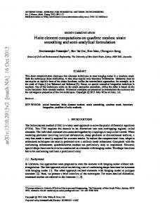
[ζj1 j2 cos 2π(j1 dk1 , j2 dk2 ) · y + ηj1 j2 sin 2π(j1 dk1 , j2 dk2 ) · y], where y = (y1 , y2 )T ∈ Ω, and dk1 and dk2 are wave number spacing and M M is the highest Fourier mode retained. The {ζj1 j2 }M j1 ,j2 =1 and {ηj1 j2 }j1 ,j2 =1 are independent standard unit Gaussian random variables. The energy spectrum of the process has exponential decay towards high frequencies. The random field b is also statistically isotropic. Figure 1 shows a realization of the random field at grid size 1/16. 2

1.5

3

1 2 1

0.5

0 −1

0

−2

−0.5

−3 −4 1

−1

0.8

4 0.6

3 0.4 y1

2 0.2

1 0

0

−1.5 y2

0

0.5

1

1.5

2 y2

2.5

3

3.5

4

Figure 1: A realization of random process bF our (y), on (y1 , y2 ) ∈ [0, 1] × [0, 4] square domain (left), and on the axis (0, y2 ) ∈ [0, 4]. The grid size is 1/16. Consider the scaled realizations δ b(y, ωi ) (i = 1, · · · , N ), δ a positive deterministic constant. We first solve (24) and obtain an approximation of the

8

principal eigenvalue µ(λ, ωi ). Then we find a sample of minimal speed c∗i (δ) = inf

λ>0

µ(λ, ωi ) λ

and the average ¯ = c∗0 + E[c∗ (δ)] ≈ E

N 1 X Mi (δ), N i=1

(26)

p where c∗0 = 2 f ′ (0) denotes the minimal speed in the case of zero advection, Mi (δ) = c∗i (δ)−c∗0 −δ¯bi and ¯bi is the integral average of b(y, ωi ) over cross section Ω. Substracting δ¯bi improves the accuracy of finite sample approximation of expectation [26, 28]. The most expensive part of the computation is solving linear eigenvalue problem (23). Due to the large number of such eigenvalue problems involved (on the scale of 104 ), the two-scale method is very helpful for reducing computational time without losing accuracy. We will solve (23) for both square and elliptical domains. We first show fully resolved computational results from the one-scale method (the standard finite element method) on the effect of domain sizes. Later, we compare these as benchmark with the results of the two-scale scheme to demonstrate the advantage of the latter. In the two-scale method, we choose the coarse mesh size H = 1/4 and the fine mesh size h = 1/16.

3.1

Resolved Computation of One-scale Method

First, we consider the square domains. We use the standard finite element method to compute the average speed with various domain aspect ratios. Figure 2 plots the ensemble averaged front speeds as a function of scaling parameter δ ∈ [0, 2] when the domains have different aspect ratios yet the same area (equal to 4). Comparing the left panel ( N = 2000) and the right panel (N = 10, 000) shows that convergence in N for averaged speeds occurs at N = 2000, in fact beginning even at N = 1000. We observe that as the domain aspect ratio increases, so does the average front speed. Because the random field b is isotropic, the average speed is invariant as the domain dimensions in y1 and y2 switch. The monotonicity of the plotted curves comes from the enhancement of front speeds by shear flows ([28] and references therein). Figure 3 plots the enhancement of the minimal speed in the range δ ∈ [0, 50]. The figure recovers the fact that when δ is small (large), the enhancement obeys a quadratic (linear) law in δ. Moreover, it shows that the effect of aspect ratio on average front speeds persists to larger values of δ. We omitted plotting the 8 × 0.5 curve partly because the 2x2 and 2.5x1.6 curves would have looked too close. We also compute the distributions of the speed enhancement M (δ) at fixed δ. We partition the range of M values into Q = 300 bins and approximate the

9

2.5

2.5 8x0.5 0.5x8 1x4 4x1 2.5x1.6 1.6x2.5 2x2

2.4

2.4

2.3

E[c (δ)]

2.2

*

*

E[c (δ)]

2.3

2.2

2.1

2.1

2

2

1.9

8x0.5 0.5x8 1x4 4x1 2.5x1.6 1.6x2.5 2x2

0

0.2

0.4

0.6

0.8

1 δ

1.2

1.4

1.6

1.8

1.9

0 2

0.2

0.4

0.6

0.8

1 δ

1.2

1.4

1.6

1.8

2

Figure 2: The average enhancement of minimal speed as a function of δ ∈ [0, 2]. Left (right) panel is with N=2000 (10,000) samples, and mesh size h=1/16. The legends show that the different lines refer to different domain aspect ratios.

speed distribution as pdf(x) =

N 1 X χj (Mi (δ)) N i=1 (xj+1 − xj )

if x ∈ [xj , xj+1 ), j = 1, · · · , Q,

(27)

where χj (x) is the characteristic function of the interval [xj , xj+1 ). Figure 4 shows the values of pdf at various domain aspect ratios with N=2000 and 10000 samples, at δ = 1. Both the mean and variance of the speed enhancement increase with the aspect ratio. Next we compute the front speeds in case of elliptical domains. The boundary equation of the elliptical domain is y2 x2 + = 1, a2 /π b2 /π where a and b are positive parameters controling the aspect ratio and area. Figure 5 shows that the average enhancement of minimal speed increases with the domain area at the same aspect ratio. Figure 6 shows the values of E[c∗ ] when 0 ≤ δ ≤ 2, and Figure 7 shows that when 0 ≤ δ < 50. The legends of these figures show the values of a, b and the number of samples.

3.2

Computations by Two-scale Method

Using the two-scale scheme, we computed the average enhancement of minimal speed with N=1000 samples in both square and elliptical domains. Choose 10

30

26 2x2 2.5x1.6 4x1

2x2 2.5x1.6 4x1 24

25

22 20

E[c (δ)]

*

*

E[c (δ)]

20 15

18 10 16

5

0

14

0

5

10

15

20

25 δ

30

35

40

45

50

12 28

30

32

34

36

38 δ

40

42

44

46

48

Figure 3: Average enhancement of minimal speed with 1000 samples.The left figure shows the values when δ ∈ [0, 50], and the right figure shows that when δ ∈ [30, 50]. The legends show that the different lines refer to different domain aspect ratios.

H = 1/4 and h = 1/16 to keep h = H 2 . In Figure 8, the fine scale corrections of step 2 and step 3 of the method clearly make an appreciable difference in averaged speeds. We see in Figure 8 that the average enhancement of minimal speed has little difference whether the domain is square shape or elliptical, as long as the area and the aspect ratio are the same. Figure 9 shows that results of the two-scale scheme agree quite well with those from the standard (one-scale) finite element discretization. Figure 10 shows that the two-scale scheme saves computing time significantly when compared with the standard finite element method. Here we use the same numerical linear algebra solver when implementing the two discretization schemes. We see in Figure 10 that the 8.0 × 0.5 square domain takes much more computing time. The reason is that for such a thin domain, the matrix condition gets worse and so the convergence rate is slower when using the inverse power method to solve the eigenvalue problem.

4

Concluding Remarks

Based on the variational principle of KPP front speeds in random shear flows in cylinders, we carried out finite element computations of KPP front speed ensemble by using both the one-scale finite element discretization and the twoscale finite element discretization. The numerically computed average speed enhancement is in agreement with theoretical analysis. In particular, equal area domains with larger aspect ratios increase the mean and variance of the front

11

18

18 2x2 2.5x1.6 4x1 8x0.5

16

14

14

12

12

10

10

8

8

6

6

4

4

2

2

0

2

2.1

2.2

2.3

2.4

2.5

2.6

2.7

2.8

2.9

2x2 2.5x1.6 4x1 8x0.5

16

3

0

*

2

2.1

2.2

2.3

2.4

2.5

2.6

2.7

2.8

2.9

3

*

c (δ), δ = 1.0

c (δ), δ = 1.0

Figure 4: Probability distribution functions of enhancement M (δ) at δ = 1.0 with N=2000 samples (left), N=10000 samples (right) for rectangular domains at four aspect ratios.

speeds in the parameter regimes simulated. The two-scale discretization scheme is much more efficient than the one-scale discretization while achieving the same accuracy. In future work, we plan to study front speed ensemble in space-time random flows [29, 31] by extending the two-scale method to parabolic problems.

5

Acknowledgments

The authors wish to thank Professor S. Shu at Xiangtan University for providing the grid generation software for elliptical domains, and the anonymous referees for their helpful suggestions.

References [1] R.A., Adams, Sobolev Spaces, Academic Press, New York, 1975. [2] R. Adler, The Geometry of Random Fields, John Wiley and Sons, 1980. [3] I. Babuska and J.E., Osborn, Finite element-Galerkin approximation of the eigenvalues and eigenvectors of selfadjoint problem, Math. Comput., 52(1989), pp. 275-297. [4] I. Babuska and J.E. Osborn, Eigenvalue problems, Handbook of numerical analysis, Vol.II, Finite element methods (Part 1) (P.G. Ciarlet and J.L. Lions, eds.), Elsevier, pp. 641-792, 1991. 12

2.07 a=4.0,b=2.0 a=2.0,b=1.0 a=1.0,b=0.5

2.06

2.05

2.04

2.03

2.02

2.01

2

1.99

0

0.1

0.2

0.3

0.4

0.5

0.6

0.7

0.8

0.9

Figure 5: The values of E[c∗ ] over elliptical domains of different areas and the same aspect ratio, with N=1000 samples.

[5] H. Berestycki, F. Hamel, and N. Nadirashvili, Elliptic eigenvalue problems with large drift and applications to nonlinear propagation phenomena, Commun. Math. Phys., 253(2005), pp. 451-480. [6] H. Berestycki and L. Nirenberg, Travelling fronts in cylinders, Ann. Inst. H. Poincare, Anal. Nonlineaire, 9(1992), pp. 497-572. [7] A. Bourlioux, B. Khouider, Rigorous asymptotic perspective on the large scale simulations of turbulent premixed flames, SIAM Multi. Modeling Simulations, 6(2007), pp 287-307. [8] S.-L. Chang, C.-S. Chien, and B.-W. Jeng, An efficient algorithm for the Schr¨ odinger-Poisson eigenvalue problem, J. Comput. Appl. Math., 205(2007), pp. 509-532. [9] F. Chatelin, Spectral Approximations of Linear Operators, Academic Press, New York, 1983. [10] M. Chertkov and V. Yakhot, Propagation of a Huygens front through turbulent medium, Phys. Rev. Lett., 80(1998), pp. 2837-2840. [11] C.-S. Chien and B.-W. Jeng, A two-grid discretization scheme for semilinear elliptic eigenvalue problems, SIAM J. Sci. Comput., 27(2006), pp. 1287-1304. 13

2.45 a = 2, b = 2,1k a = 2, b = 2, 5k a = 2, b = 2, 10k a = 2.5, b = 1.6, 1k a = 2.5, b = 1.6, 5k a = 2.5, b = 1.6,10k a = 4, b = 1, 1k a = 4, b = 1, 5k a = 4, b = 1, 10k a = 8, b = 0.5, 1k a = 8, b = 0.5, 5k a = 8, b = 0.5, 10k

2.4

2.35

2.3

2.25

25 a=2, b=2, 10k a = 2.5,b = 1.6,10k a = 4, b = 1, 10k

20

E[c*(δ)]

E[c*(δ)]

15 2.2

2.15 10 2.1

2.05 5 2

1.95

0

0.2

0.4

0.6

0.8

1 δ

1.2

1.4

1.6

1.8

Figure 6: The values of E[c∗ ] with different domain aspect ratios and the same area, at δ ∈ [0, 2], N=1000, 5000 and 10,000 samples.

2

0

0

5

10

15

20

25 δ

30

35

40

45

Figure 7: The values of E[c∗ ] with different domain aspect ratios and the same area, at δ ∈ [0, 50], N=10,000 samples.

[12] P.G. Ciarlet, The Finite Element Method for Elliptic Problems, NorthHolland, Amsterdam, New York, Oxford, 1978. [13] P.G. Ciarlet and J.L. Lions, Handbook of Numerical Analysis, Vol.II, Finite Element Methods (Part I), North-Holland, 1991. [14] P. Clavin and F. Williams, Theory of premixed-flame propagation in largescale turbulence, J. Fluid Mech., 90(1979), pp. 598-604. [15] P. Constantin, A. Kiselev, A. Oberman, and L. Ryzhik, Bulk burning rate in passive-reactive diffusion, Arch. Rat. Mech. Anal., 154(2000), pp. 53-91. [16] J. G¨ artner and M. Freidlin, The propagation of concentration waves in periodic and random media, Dokl. Acad. Nauk. SSSR, 249(1979), pp. 521525. [17] F. Hamel, Formules min-max pour les vitesses d’ondes progressives multidimensionnelles, Ann. Fac. Sci. Toulouse, 8(1999), pp. 259-280. [18] S. Heinze, G. Papanicolaou, and A. Stevens, Variational principles for propagation speeds in inhomogeneous media, SIAM J. Applied Math, 62(2001), pp. 129 - 148. [19] A. R. Kerstein and W. T. Ashurst, Propagation rate of growing interfaces in stirred fluids, Phys. Rev. Lett., 68(1992), pp. 934-937.

14

50

2.6

2.6 2x2,H 2x2,h 2.5x1.6,H 2.5x1.6,h 4.0x1.0,H 4.0x1.0,h 8.0x0.5,H 8.0x0.5,h

2.5

2.4

2x2, H 2x2, h 2.5x1.6, H 2.5x1.6, h 4.0x1.0, H 4.0x1.0, h 8.0x0.5, H 8.0x0.5, h

2.5

2.4

*

*

E[c (δ)]

2.3

E[c (δ)]

2.3

2.2

2.2

2.1

2.1

2

2

1.9

0

0.2

0.4

0.6

0.8

1 δ

1.2

1.4

1.6

1.8

2

1.9

0

0.2

0.4

0.6

0.8

1 δ

1.2

1.4

1.6

1.8

2

Figure 8: The average enhancement of minimal speed with N=1000 samples, computed by the two-scale scheme. The left panel shows the enhancement of speed in the coarse mesh (results by step 1 in the two-scale scheme) and after the fine mesh correction (results by step 2 and step 3 in the two-scale scheme) for the square domain. The right panel is for the elliptical domain.

[20] K. Kolman, A two-level method for nonsymmetric eigenvalue problems, Acta Math. Appl. Sinica, 21(2005), pp. 1-12. [21] P.R. Kramer, A review of some Monte Carlo simulation methods for turbulent systems, Monte Carlo Methods and Applications, 7(2001), pp 229-244. [22] Q. Lin, Some problems concerning approximate solutions of operator equations, Acta Math. Sinica, 22(1979), pp. 219-230 (in Chinese). [23] Q. Lin and G. Xie, Accelerating the finite element method in eigenvalue problems, Kexue Tongbao, 26(1981), pp. 449-452 (in Chinese). [24] F. Liu and A. Zhou, Two-scale finite element discretizations for parallel differential equations, J. Comput. Math., 24(2006), pp 373-392. [25] A. Majda and P. Souganidis, Flame fronts in a turbulent combustion model with fractal velocity fields, Comm. Pure Appl. Math., 51(1998), pp. 13371348. [26] J. Nolen and J. Xin, Variational principle based computation of KPP average front speeds in random shear flows, Methods Appl. Anal., 11(2004), No. 3, pp. 389-398. [27] J. Nolen, J. Xin, Min-Max Variational Principle and Front Speeds in Random Shear Flows, Methods Appl. Anal., 11(2004), No. 4, pp. 635-644.

15

[28] J. Nolen and J. Xin, A variational principle based study of KPP minimal front speeds in random shears, Nonlinearity, 18(2005), pp. 1655-1675. [29] J. Nolen and J. Xin, Variational principle of KPP front speeds in temporally random shear flows with applications, Comm. Math. Phys., 269(2007), pp. 493-532. [30] J. Nolen and J. Xin, Computing Reactive Front Speeds in Random Flows by Variational Principle, Physica D, to appear, 2008. [31] J. Nolen and J. Xin, Asymptotic spreading of KPP reactive fronts in incompressible space-time random flows, to appear in Ann l’Inst. Henri Poincar´e, Analyse Nonlineare, 2008. [32] P. Ronney, Some open issues in premixed turbulent combustion, in: Modeling in Combustion Science (J. D. Buckmaster and T. Takeno, Eds.), Lecture Notes in Physics, Vol. 449, Springer-Verlag, Berlin, pp. 3-22, 1995. [33] P. Ronney, B. Haslam, N. Rhys, Front propagation rates in randomly stirred media, Phys. Rev. Lett., 74(1995), pp. 3804-3807. [34] L. Shen, Parallel Adaptive Finite Element Algorithms for Electronic Structure Computing based on Density Functional Theory, PhD Thesis, Academy of Mathematics and Systems Science, Chinese Academy of Sciences, 2005. [35] I. H. Sloan, Iterated Galerkin method for eigenvalue problems, SIAM J. Numer. Anal., 13(1976), pp. 753-760. [36] J. Xin, Front propagation in heterogeneous media, SIAM Rev., 42, 2000, pp 161-230. [37] J. Xin, KPP front speeds in random shears and the parabolic Anderson problem, Methods Appl. Anal., 10(2003), pp. 191-198. [38] J. Xu and A. Zhou, A two-grid discretization scheme for eigenvalue problems, Math. Comput., 70(2001), pp. 17-25. [39] V. Yakhot, Propagation velocity of premixed turbulent flames, Comb. Sci. Tech., 60(1988), pp. 191-214. [40] A. Zlatos, Pulsating front speed-up and quenching of reaction by fast reaction, Nonlinearity 20(2007), pp 2907-2921.

16

2.6 2x2, 2−scale 2x2, 1−scale 2.5x1.6, 2−scale 2.5x1.6,1−scale 4x1, 2−scale 4x1,1−scale 8x0.5, 2−scale 8x0.5, 1−scale

2.5

2.4

E[c*(δ)]

2.3

2.2

2.1

2

1.9

0

0.2

0.4

0.6

0.8

1 δ

1.2

1.4

1.6

1.8

2

Figure 9: The average enhancement of minimal speed computed with the fine mesh h = 1/16. The data points from the two-scale method come close to those from the standard finite element method. 4

8

x 10

1−scale, h 2−scale, h

7

6

CUP time (secs.)

5

4

3

2

1

0 2x2

2.5x1.6

4x1

8x0.5

Figure 10: The time used to produce the data in Figure 9 by one-scale and two-scale methods.

17