FPGA based Implementation of Image Quality Measures

International Journal of Computer Applications (0975 – 8887) Volume 176 – No.4, October 2017

FPGA based Implementation of Image Quality Measures: A Comprehensive Approach Sarmad F. Ismael

Yahya T. Qassim, PhD School of Electronic Engineering Griffith University Brisbane- Australia

Electronic Engineering Department Nineveh University Mosul- Iraq

ABSTRACT This paper presents the design and implementation of six Image quality measures used to investigate the similarity between reconstructed images (after Denoising process) and the original ones on Spartan 3E XC3S500E FPGA. Since the visual comparison is too subjective, objective measure of image quality is required. The objective measure takes advantage of the variance in the statistical distribution of the coefficients in the image. The designed architecture was tested using five gray scale (128 x 128) images and it runs properly at a maximum clock rate of 70.74 MHz. By employing a parallel architecture, the speed performance has increased to 1064 times in comparison to Matlab running time.

designed FPGA architecture. In Section III, the implementation of the design and implications are outlined whereas Section IV presents the results and Section V conclude this work.

2. METHODS Some of the most popular image quality measures that are implemented using FPGA in this paper are the Normalized Mean Square Error (NMSE), Normalized Average Difference (NAD), Maximum Difference (MD), Normalized CrossCorrelation (NK), Normalized Absolute Error (NAE) and the Structural Content (SC) [3]. These measures are formulated as follows:

General Terms Computer architecture, computational technology.

Keywords Image quality, FPGA, Accumulators, parallel processing.

1. INTRODUCTION Image quality assessment has been widely used to investigate the degradation in images reconstructed through digital communication and processing. Many efficient measures with different features have been developed to overcome the shortness in any single method applied in digital photography and to show deeper indication on the similarity between the original image and the one derived from the original [1]. The increase in digital imaging throughout the world and in the United States of America in particular arise the need to improve the speed of quality assessment of those images [2]. Previous works have handled the image quality algorithms, analysis and software processing [1]-[6]. In [1], [4], Image quality methods where used to investigate the quality of reconstructed images from compression, whereas in [5], the quality measures were employed to examine the closeness between the wavelet coherence (coherogram figures) implemented in hardware and the ones implemented in Matlab. However, to the best of authors’ knowledge, hardware implementation of image quality measures has not been addressed in the literature. In general, the image quality assessment can be classified into subjective assessment and objective assessment [2]. The slowness and low quality in the subjective assessment of digital images reduce the reliability of this classification and lead to the development of several objective measures. However, due to the huge number of digital images that need to be processed, hardware involvement is crucial to speed up the process since the hardware is many times faster in computation compared to the software. The remainder of this paper is organized as follows, Section II introduces the image quality measures utilized in this paper and the change made in the equations’ formula to serve the

Where,

is the sample of the original image field and denotes the sample of the reconstructed image field.

The quality measures of (1-6) are all bivariate and discrete, which means they provide the mechanism of exploiting the differences between the values of pixels represented by their statistical distributions [3]. In order to be FPGA implementation-ready, both of (1) and (2) are re-formulated as:

(7)

It can be noticed that some operations are common between image quality measures in (3)-(8); therefore, the next step is to extract and calculate the terms and common operations between these measures. Table 1 lists those common

42

International Journal of Computer Applications (0975 – 8887) Volume 176 – No.4, October 2017 operations versus each method. The common operations are highly regarded to avoid the repetition in FPGA computation. Table 1. The operations employed in image quality measures and the common operations #

Operation

Employment

1.

NAD, NK, NAE, SC, NMSE

2.

NK, SC, NMSE

3.

NK, SC, NMSE, NAD

4.

SC, NMSE

5.

NK, NMSE

6.

NAE

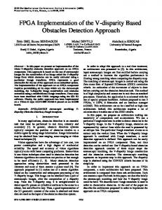
3.2 Block 2 This block start computing the assigned formulas that are analyzed (3)-(8). It is worthwhile to mention that all terms are computed as parts of the six measures in the architecture. The accumulators were considered as a major part of this block since all formulas contain accumulation (see Figure 1). The used accumulators here are of two configurations: the general accumulator (GAC) and the multiplier accumulator (MAC). The accumulator accumulates the input data at each clock pulse when using the GAC. Otherwise, the input data is multiplied with another input set before accumulation when the MAC is employed. Figure 2 shows the MAC configuration (the GAC is the same configuration excluding the multiplier). In order to receive a new input data, the clear (CLR) pin in the MAC is provided to clear the output data.

DIN1

Nbit Re gis ter

DIN2

3. FPGA IMPLEMENTATION The image quality architecture (Figure 1) was designed using VHDL language and it considers all formulas (1)-(6) outlined in this paper. From Figure 1, the overall image quality architecture consists of four blocks; each block is explained in detail as follows.

DOUT

CLK CLR

Fig.2: The MAC Unit. DIN1 & DIN2 are Inputs, DOUT is Output.

2Kx8 for original image (128x128)

2Kx8 for reconstructed image (128x128) Block1

Addition, subtraction and division operation

MUX circuit to select the specified image quality measure

Block3

Block4

Output of measure

Block2 Fig.1: Block Diagram for the Architecture of Image Quality Measures

3.1 Block 1 In block 1, each of the original and reconstructed images (128 x 128= 16384 total pixels) were stored in eight block RAMs (on-chip memory), each of size 2Kx 8 bit (1 byte/pixel) as a pre-processing step (total BRAM required 16 x2K for both images). For this number of pixels, 14-bit address bus is needed; 11-bit to address each of the eight 2K memories and the rest of 3-bit addresses are used as selectors for an 8x1 multiplexer circuit. The multiplexer circuit specifies which pixel is going to be fetched from the assigned memory. Fetching a pixel from the original image and the corresponding pixel from the reconstructed image occurs at the same time.

3.3 Block 3 In block three, the operations of addition, subtraction and division were performed on the coming data from block 2 to produce the final image quality measure. The direct implementation of division in VHDL can be achieved in simulation. However, it cannot be synthesized or implemented. Therefore, we have searched for an algorithm suitable for large number of accumulator bits as in our case. The non-restoring algorithm was found and employed due to its suitability [7]. In this method of division, the result can be obtained in one clock pulse only; however, it needs extra FPGA logic slices when compared to the direct division. At this block, the output results of the six image quality measures are available.

43

International Journal of Computer Applications (0975 – 8887) Volume 176 – No.4, October 2017

3.4 Block 4

4. RESULTS AND DISCUSSION

The last block of Figure 1 is the multiplexing circuit. It is utilized to select the denoted image quality measure through an 8x1 multiplexer. Table 2 shows the image quality output according to the input selector.

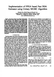
As mentioned in the introduction, the quality measure shows the amount of closeness between the original image and the impaired one. This section presents the result of image quality measures for five gray-scale images performed in both Matlab and FPGA and shows the comparison. The five (128x128) images used are: Baboon, Barbara, Cameraman, Goldhill and Peppers (see Figure 3).

Table 2. Image quality selection according to input Selector (2) 0 0 0 0 1 1

Selector (1) 0 0 1 1 0 0

Selector (0) 0 1 0 1 0 1

Output measure NMSE NAD MD NK NAE SC

The total number of clock cycles required for parallel execution of all measures in the architecture is 16385 clock. A careful consideration of bit resolution (the integer; including the sign bit and the fraction part) for each term has been considered to achieve maximum accuracy of results. Therefore, for the six image quality measures, the number of bit used is listed in Table 3 in details. The fixed-point package [8] is used to represent variables in the VHDL code. The 2’S complement number representation was used to represent the pixels of the images employed. Table 3. Number of bit required for each measure Image quality measure NMSE NAD MD NK NAE SC

Total No. of bit 39 31 8 39 31 39

Integer part (including sign bit) 31 23 8 31 23 31

Fraction part 8 8 0 8 8 8

The allocated high number of bit in the FPGA design was necessary to obtain sufficient accuracy for the results. Hence, both of the Matlab results and the FPGA results were experienced along the list of operations in Table 1 and compared. The FPGA calculation gives the same output result compared to Matlab as shown in Table 4. The original standard image used here and its reconstructed counterpart is the “Baboon”. The terms presented in Table 4 are calculated in Figure 1- block 2. It can be noticed that most values in Table 4 are large numbers because of the summation process, and this explains why the total number of bit chosen was high. Table 4. Comparison between the outputs of Fig.1 (block2) performed in software and hardware for the Baboon image Summation Term

Matlab calculation 2136986 298989686 2126994 295628230 295084896 151592

FPGA calculation 2136986 298989686 2126994 295628230 295084896 151592

(a)

(b)

(c)

Fig.3: The five standard images used for testing the architecture of image quality. (a) Original images, (b) noise added to images, (c) reconstructed images. Column (a) & (c) used to test the FPGA architecture. A Gaussian white noise was added to each of the original images in Figure 3-(a) and resulted the images in Figure 3-(b). With a Denoising process, the set of images in Figure 3-(c) were produced. The reconstructed images subjectively show impairment compared to the originals. However, for accurate measure, objective methods were employed. Columns (a) and (c) of Figure 3 were used to find each of the mentioned image quality measures in software and FPGA. The result of image quality calculation were listed in Table 5 for both software and hardware; in decimal and hexadecimal radix as well for the six measures. Table 5 presents the image quality measures for the five images where each of the normalized method: NMSE, NAD, NAE are close to zero, NK and SC are around 1 and MD gives the maximum difference. Acronyms were added to differentiate between measures, where “Bab” stands for “Baboon”, “Bar” for ”Barbara”, “Cam” for “Cameraman”, “Gol” for “Goldhill” and “Pep” for “Peppers”. There is a high closeness between the Matlab and

44

International Journal of Computer Applications (0975 – 8887) Volume 176 – No.4, October 2017 the FPGA computation, which proves the correctness of the calculations performed in hardware. Table 5. Image quality measures performed in software and hardware for five images, “Bab” for Baboon, “Bar” for Barbara, “Cam” for Cameraman, “Gol” for Goldhill and “Pep” for Peppers. Img

Bab

Bar

Cam

Gol

Pep

Measure NMSE NAD MD NK NAE SC NMSE NAD MD NK NAE SC NMSE NAD MD NK NAE SC NMSE NAD MD NK NAE SC NMSE NAD MD NK NAE SC

Matlab result Decimal Hex 0.0149 0.03D 0.0047 0.013 205 CD.0 0.9869 0.FCA 0.0709 0.122 1.0114 1.02E 0.0152 0.03E 0.0068 0.01B 217 D9 0.9861 0.FC7 0.0577 0.0EC 1.0127 1.034 0.0212 0.056 0.0075 0.01E 246 F6 0.9821 0.FB6 0.0638 0.105 1.0147 1.03C 0.0109 0.02C 0.0029 0.00BE 245 F5 0.9913 0.FDC 0.0512 0.0D1 1.0066 1.01B 0.0143 0.03A 0.0065 0.01A 226 E2 0.9867 0.FC9 0.0509 0.0D1 1.0125 1.004

FPGA result Decimal Hex 0.0117 0.03 0.0078 0.02 205 CD.0 0.9843 0.FC 0.0703 0.12 1.0117 1.02 0.0117 0.03 0.00781 0.02 217 D9 0.9844 0.FC 0.0547 0.0E 1.0117 1.03 0.0195 0.05 0.0078 0.02 246 F6 0.9804 0.FB 0.0625 0.10 1.0117 1.03 0.0078 0.02 0.0039 0.01 245 F5 0.9882 0.FD 0.0507 0.0D 1.0039 1.01 0.0117 0.03 0.0078 0.02 226 E2 0.9843 0.FC 0.0507 0.0D 1.0117 1.03

For all images in Table 5, despite the sufficient number of bits employed (for the integer and fraction parts) to calculate the quality measures in FPGA, there are still small differences between hardware and software results (excluding the MD measure). This is because of the effect of the quantization error. The quantization error appeared when numbers were converted to hexadecimal. Figure 4 shows the final section of the timing simulation for the “Baboon” image. Figure 4 displays the waveforms for the last stage of the image quality measures applied to the “Baboon” image. The duration of the clock cycle is 10 ms and the represented numbers are real numbers where the position of the decimal point has been assigned in advance. The total number of clock cycles required to calculate and produce all measures was 16385 clock. The maximum operational frequency for this architecture according to its critical path is 70.746 MHz. Therefore, the FPGA execution time can be calculated as:

Fig.4: The timing simulation to produce the quality measures for the Baboon image The average time to calculate the same computations in Matlab is 0.2457 sec on a laptop machine provided with core i5 cpu @ 2.4 GHz, 8 GB RAM, SSD HDD and running Windows 10. Hence, the speed-up ratio obtained can be calculated as:

= 0.2457 sec/ 231.603 μ sec = 1061 times. The entire image quality architecture was implemented on Xilinx Spartan 3E XC3S500E FPGA using ISE14.7 simulator [9]. The synthesis step of the design produces the utilized resources from the FPGA chip and these are listed in Table 6. Table 6. The summary of FPGA resources utilization Logic utilization

Used

Available

Utilization

Number of Slices

3703

4656

79%

Number of Slice FF

346

9312

3%

Number of LUTs

7288

9312

78%

Number of IOBs

44

232

18%

Number of BRAMs

16

20

80%

Number of Multipliers

3

20

15%

Number of GCLKs

1

24

4%

5. CONCLUSIONS The presented architecture for image quality measures produces the results of six measures for two input (128x128) gray scale images in high calculation speed and high frequency of Spartan 3E chip. Despite the extensive area utilized of Spartan 3E (up to 80%), the maximum operational frequency was as high as 70.746 MHz. With a sufficient number of bits used for representing inputs and internal signals, reasonable accuracy was obtained when the design was tested with five standard images and compared to Matlab. The total number of clock cycles required to calculate the six measures was 16385 and the total FPGA time to calculate all measures was as short as 231.6 μ sec. This speed is more than 1000 times faster than Matlab computation. The future scope of the presented work is to utilize the designed architecture in real time applications of image quality measures involving the FPGA as a target platform. The obtained FPGA processing speed in the outlined work supports this notion.

= 16385/ 70.746 MHz = 231.603 μ sec.

45

International Journal of Computer Applications (0975 – 8887) Volume 176 – No.4, October 2017

6. REFERENCES [1] Eskicioglu, A. and Fisher, P. 1993. A survey of quality measures for gray scale image compression. 9th Computing in Aerospace Conference, 49-61. [2] K. Gu, G. Zhai, X. Yang, W. Zhang, “Using free energy principle for blind quality assessment”, IEEE Transactions on Multimedia, 2015, Vol. 17, No. 1, 5063. [3] Eskicioglu, A. and Fisher, P., “Image quality measures and their performance”, IEEE Transactions on Communications, 1995, Vol. 43, No. 12, 2959-2965. [4] Poopal S. and Ravindran G., “The performance of fractal image compression on different imaging modalities using objective quality measures”, International Journal of Engineering Science and Technology, 2011, Vol. 3, No. 1, 525-530. [5] Qassim, Y., Cutmore T. and Rowlands, D., “FPGA implementation of wavelet coherence for EEG and ERP

IJCATM : www.ijcaonline.org

signals”, Microprocessors and Microsystems, 2017, Vol. 51, 356-365. [6] Fang R., Al-Bayaty R. and Wu, No-Reference Image Quality Transactions on Circuits and Technology, 2015, TCSVT.2016.2539658.

D., “BNB Method for Assessment”, IEEE Systems for Video DOI: 10.1109/

[7] B. Jovanovic and M. Jevtiv, 2010, FPGA Implementation of Throughput Increasing Techniques of The Binary Dividers, international scientific conference, 397-401, 19-20. [8] D. Bishop, 1076-2008 Fixed point package user’s guide. Packages and bodies for the IEEE. [9] Ismael, S. and Mahmod, B., “A novel way to design and implement statistical operations based on FPGA”, International Journal of Computer Applications, 2017, Vol. 167, No. 9, 8-11.

46