fully parallel learning neural network chip for real

FULLY PARALLEL LEARNING NEURAL NETWORK CHIP FOR REAL-TIME CONTROL

A Thesis Presented to the Academic Faculty In Partial Fulfillment of the Requirements for the Degree of Doctor of Philosophy in Electrical Engineering

By Jin Liu

School of Electrical and Computer Engineering Georgia Institute of Technology May 25, 1999 Copyright  1999 by Jin Liu

FULLY PARALLEL LEARNING NEURAL NETWORK CHIP FOR REAL-TIME CONTROL

Approved:

______________________________ Martin A. Brooke

______________________________ Stephen DeWeerth

______________________________ Thomas Habetler

Date: ______________________________

ii

DEDICATION

To my family: My mother, Kuiying Zhang My father, Peiran Liu My sister, Yue Liu And my husband Jian Dong For their love, inspiration, and believing

iii

ACKNOWLEDGEMENT I would like to thank my thesis advisor, Dr. Martin Brooke, for giving me the opportunity to pursue my dream, for his encouragement and believing. I appreciate the four years under his guidance. I was inspired by his knowledge, wisdom, and more important, by his great character, his generosity, his attitude for research and life, which will benefit me for lifetime. I would like to thank Dr. Phillip Allen. He taught most of my analog IC design classes. His seriousness in research and teaching inspire me to strive and achieve. I would like to thank Dr. Stephen DeWeerth and Dr. Thomas Habetler for serving as my thesis reading committee member, for the constructive comments and supports. I would like to thank Dr. Umakishore Ramachandran for serving on my defense committee, for the computer science knowledge learned from him, and for his patience and encouragement. I like to thank all the group members for their constant help and friendship. Special thanks to Sungyoung Jung, Youngjoong Joo, Jaejoon Chang, Jinsung Park, Ravi Poddar, Larry Carastro, and John Tabler. I like to thank all my friends in Atlanta. Their friendship, love, and companion helped me go through the years of my graduate study, with special thanks to Liang Chen, Nanju Na, Sean Xie, Sumei Lin, Alex Zhao, Denny Yeung etc.

iv

I like to thank my family friend Chang Wang and his family for caring me as a daughter. I like to thank my mom Kuiying Zhang for her love, her constant support, and her friendship.

I like to thank my father Peiran Liu and my sister Yue Liu for their

unconditional love. And I like to thank my husband Jian Dong for his love, support and patience during my Ph. D. work.

v

TABLE OF CONTENTS

DEDICATION ..........................................................................................................................................III

ACKNOWLEDGEMENT........................................................................................................................IV

TABLE OF CONTENTS .........................................................................................................................VI

LIST OF TABLES ..................................................................................................................................... X

LIST OF FIGURES ................................................................................................................................ XII

SUMMARY............................................................................................................................................ XVI

CHAPTER I INTRODUCTION................................................................................................................ 1 1.1 BACKGROUND REVIEW ........................................................................................................................1 1.2 THESIS ORGANIZATION ........................................................................................................................4 CHAPTER II LITERATURE REVIEW .................................................................................................. 6 2.1 NEURAL NETWORK IMPLEMENTATIONS ...............................................................................................6 2.2 BASICS OF NEURAL NETWORKS .........................................................................................................21 2.3 LEARNING NEURAL NETWORK CHIPS IN LITERATURE........................................................................22 2.4 APPLICATION AREAS OF LEARNING NEURAL NETWORK CHIPS IN LITERATURE .................................53 CHAPTER III REAL-TIME CONTROL WITH HARDWARE NEURAL NETWORK ................. 55 3.1 REAL-TIME CONTROL SCHEME ..........................................................................................................55 3.2 APPLICATION OF NEURAL NETWORKS FOR REAL-TIME CONTROL ......................................................56 3.3 ISSUES FOR HARDWARE NEURAL NETWORKS ....................................................................................57

vi

CHAPTER IV EFFECTS OF ANALOG CIRCUIT NONIDEALITY ................................................ 60 4.1 THE INDUCTION MOTOR APPLICATION ..............................................................................................60 4.2 ANALOG CIRCUIT NONIDEALITY AND SIMULATION RESULT...............................................................63 CHAPTER V COMBUSTION INSTABILITY PROBLEMS .............................................................. 68

CHAPTER VI SOFTWARE SIMULATION OF COMBUSTION INSTABILITY CONTROL...... 72 6.1 INTRODUCTION ..................................................................................................................................72 6.2 UNDAMPED OSCILLATORY PLANT .....................................................................................................74 6.3 BOUNDED UNDAMPED OSCILLATORY PLANT ....................................................................................81 CHAPTER VII PRELIMINARY HARDWARE TESTS AND MODIFICATIONS .......................... 99 7.1 INTRODUCTION ..................................................................................................................................99 7.2 THE RWC CHIP ...............................................................................................................................100 7.3 INITIAL MODIFICATIONS AND SPICE SIMULATIONS ...........................................................................104 7.4 TEST PREPARATIONS .......................................................................................................................107 7.5 SHIFT REGISTERS .............................................................................................................................109 7.6 MULTIPLIERS ...................................................................................................................................110 7.7 THE WEIGHT UPDATING ..................................................................................................................112 7.8 TRAINING ONE WEIGHT ...................................................................................................................115 7.9 TWO-INPUT INVERTER .....................................................................................................................120 7.10 CONCLUSION..................................................................................................................................129 CHAPTER VIII HARDWARE CONTROL OF COMPUTER SIMULATED PLANT .................. 130 8.1 TEST SETUP .....................................................................................................................................130 8.2 TEST RESULTS .................................................................................................................................132 8.3 RESULTS WITH LONGER RUNNING TIME ..........................................................................................140 8.4 RESULT WITH BIGGER DAMPING FACTORS.......................................................................................142

vii

CHAPTER IX DESIGN OF AN IMPROVED LEARNING NEURAL NETWORK CHIP ............ 146 9.1 THE CHIP ARCHITECTURE ................................................................................................................146 9.2 DESIGN OF THE WEIGHT CELL .........................................................................................................150 9.3 SPICE SIMULATIONS .........................................................................................................................152 CHAPTER X CONCLUSION AND FUTURE WORK ...................................................................... 159 10.1 SUMMARY OF RESEARCH ...............................................................................................................159 10.2 FUTURE WORK ..............................................................................................................................160 10.3 CONCLUSION..................................................................................................................................161 APPENDIX A.1 NONLINEAR MULTIPLIER SIMULATION CODE............................................ 163

APPENDIX B.1 UNBOUNDED OSCILLATOR-ONE FREQUENCY ............................................. 184

APPENDIX B.2 UNBOUNDED OSCILLATOR-TWO FREQUENCY ............................................ 192

APPENDIX B.3 LIMIT CYCLE OSCILLATOR-ONE FREQUENCY............................................ 200

APPENDIX B.4 LIMIT CYCLE OSCILLATOR-VARIABLE PLANT PARAMETERS .............. 209

APPENDIX B.5 LIMIT CYCLE OSCILLATOR-NOISE ADDED ................................................... 222

APPENDIX C.1: SPICE SIMULATION CODES ............................................................................... 236

APPENDIX C.2: THE HARDWARE SPECIFICATIONS................................................................. 238

APPENDIX C.3: DATA ACQUISITION CARD SETUP AND PROGRAMMING ........................ 239

APPENDIX C.4: THE OPAMP CIRCUIT FOR CURRENT TO VOLTAGE TRANSFORMATION .................................................................................................................................................................. 242

APPENDIX C.5: MEASUREMENT OF THE CHIP WHEN POWERED UP................................. 244

viii

APPENDIX C.6: TEST CODE IN BORLAND C++ ........................................................................... 246

APPENDIX C.7: TEST RESULT FOR THE SHIFT REGISTER..................................................... 271

APPENDIX C.8: MORE DATA FOR INVERTER TESTING .......................................................... 288

APPENDIX D.1: THE PIN ASSIGNMENT OF AT-AO-10 ............................................................... 291

APPENDIX D.2: THE TEST PROCEDURE FOR THE NEURAL NETWORK CHIP CONTROL OF SIMULATED COMBUSTION ....................................................................................................... 292

APPENDIX D.3: THE TEST CODE IN BORLAND C/C++ FOR THE NEURAL NETWORK CHIP CONTROL OF SIMULATED COMBUSTION .................................................................................. 293

APPENDIX E.1 SPICE SIMULATION CODE FOR THE IMPROVED CHIP .............................. 306

REFERENCES........................................................................................................................................ 311

VITA...........................................................................................................................................................316

ix

LIST OF TABLES TABLE 1: TIME .............................................................................................................................................10 TABLE 2: CHIP AREA (GATE NUMBERS).......................................................................................................12 TABLE 3: ESTIMATED CHIP AREA FOR THE FULLY PARALLEL ANALOG IMPLEMENTATION ...........................12 TABLE 4: EFFICIENCY ...................................................................................................................................13 TABLE 5: TIME IN THE 0.35-µM CMOS PROCESS (NS)..................................................................................15 TABLE 6: CHIP AREA IN THE 0.35-µM CMOS PROCESS (MM2) ......................................................................16 TABLE 7: TIME IN THE 70-NM CMOS PROCESS (NS).....................................................................................18 TABLE 8: CHIP AREA IN THE 70-NM CMOS PROCESS (MM2) .........................................................................19 TABLE 9: COMPARISON OF DIFFERENT NETWORK MODELS..........................................................................33 TABLE 10: COMPARISON OF FIVE KINDS OF WEIGHT STORAGE CIRCUITS ....................................................51 TABLE 11: THE ζ VALUES ............................................................................................................................76 TABLE 12: CHIP PIN ASSIGNMENT ..............................................................................................................103 TABLE 13: NATIONAL INSTRUMENT AT-MIO-16E-2 .................................................................................108 TABLE 14: NATIONAL INSTRUMENT AT-AO-10 .........................................................................................108 TABLE 15: A CHOSEN SET OF VOLTAGE BIASES.........................................................................................112 TABLE 16: PARAMETERS FOR THE RESULT SHOWN IN FIGURE 66 ...............................................................132 TABLE 17: PARAMETERS - FREQUENCY AND DAMPING FACTOR ................................................................142 TABLE 18: ASSIGNMENTS FOR THE TOP PADS OF THE CHIP ........................................................................149 TABLE 19: INTERFACE BETWEEN THE AT-MIO-16E-2 CARD AND THE CHIP..............................................240 TABLE 20: USAGE OF THE DIO PORTS .......................................................................................................240 TABLE 21: TEST RESULT OF THE CURRENT TO VOLTAGE CONVERSION WITH OPAMP ................................243 TABLE 22: POWER UP MEASUREMENT .......................................................................................................244

x

TABLE 23: VOLTAGE BIASES FOR MULTIPLIER TEST ..................................................................................244 TABLE 24: THE OUTPUT CURRENT AS A FUNCTION OF THE POSITIVE POWER SUPPLY................................245 TABLE 25: THE OUTPUT CURRENT AS A FUNCTION OF VOLTAGE BIAS ......................................................245 TABLE 26: THE OUTPUT CURRENT IS REVERSED WITH A HIGH ("1") SHIFTED IN. ......................................245

xi

LIST OF FIGURES FIGURE 1: TIME ............................................................................................................................................11 FIGURE 2: CHIP AREA (GATE NUMBERS)......................................................................................................13 FIGURE 3: EFFICIENCY ..................................................................................................................................14 FIGURE 4: AREA AND TIME REQUIREMENT FOR DIFFERENT IMPLEMENTATION METHODS WITH DIFFERENT NEURAL NETWORK SIZES FOR 0.35-µM CMOS PROCESS.............................................................................17 FIGURE 5: CUBIC SPLINE INTERPOLATION OF THE 31-STAGE RING OSCILLATOR FREQUENCY IN 70-NM CMOS PROCESS .......................................................................................................................................................18 FIGURE 6: AREA AND TIME REQUIREMENT FOR DIFFERENT IMPLEMENTATION METHODS WITH DIFFERENT NEURAL NETWORK SIZES FOR 70-NS CMOS PROCESS.................................................................................20 FIGURE 7: A NEURON ...................................................................................................................................21 FIGURE 8: THE TWO-LAYER FEED-FORWARD NEURAL NETWORK ARCHITECTURE ......................................23 FIGURE 9: THE CHIP ARCHITECTURE OF ONE LAYER NETWORK IN A MULTILAYER NEURAL NETWORK.......24 FIGURE 10: THE ARCHITECTURE OF A FULLY CONNECTED NETWORK, WITH INPUT, HIDDEN AND OUTPUT NEURONS [23] ..............................................................................................................................................30 FIGURE 11: THE KOHONEN NETWORK .........................................................................................................31 FIGURE 12: THE ONE-DIMENSIONAL KOHONEN NETWORK ARCHITECTURE .................................................32 FIGURE 13: THE WEIGHT STORAGE AND MODIFICATION CIRCUIT [23].........................................................36 FIGURE 14: THE WEIGHT STORAGE AND MODIFICATION CIRCUIT [22].........................................................38 FIGURE 15: THE WEIGHT STORAGE AND MODIFICATION CIRCUIT [25].........................................................39 FIGURE 16: THE WEIGHT STORAGE CIRCUIT AND THE MULTIPLIER CIRCUIT [12] ........................................41 FIGURE 17: THE SCHEMATIC OF THE SYNAPSE CIRCUIT [16]........................................................................42 FIGURE 18: SYNAPSE WEIGHT UPDATE SCHEME [19]...................................................................................46 FIGURE 19: MULTIPLIER CIRCUIT WITH 4-BIT CONNECTION WEIGHT [43] ....................................................47

xii

FIGURE 20: DIGITAL STORAGE FOR DIGITAL/ANALOG HYBRID SYNAPSE [44] ..............................................48 FIGURE 21: ANALOG EXTENSION OF A MIXED ANALOG/DIGITAL WEIGHT [44].............................................49 FIGURE 22: A NEURAL NETWORK CONTROLLER ..........................................................................................55 FIGURE 23: RELATIONSHIP BETWEEN THE STATOR VOLTAGE, CURRENT, SHAFT TORQUE AND SPEED.........61 FIGURE 24: SIMULATION RESULT OF INDUCTION MOTOR USING THE RWC ALGORITHM .............................63 FIGURE 25: IDEAL MULTIPLIER AND THE ONE-SIDED NONLINEAR MULTIPLIER. ...........................................64 FIGURE 26: MULTIPLIER MEASURED FROM THE RWC CHIP .........................................................................65 FIGURE 27: SIMULATION RESULTS OF IDEAL MULTIPLIERS AND NONIDEAL MULTIPLIERS ............................66 FIGURE 28: THE NEURAL NETWORK CONTROL OF UNSTABLE COMBUSTION ENGINE SYSTEM .....................73 FIGURE 29: THE RESULTS OF THE SIMULATED HARDWARE NEURAL NETWORK CONTROLLER.....................77 FIGURE 30: COMBUSTION MODEL WITHOUT THE NEURAL NETWORK CONTROL ..........................................78 FIGURE 31: REDRAW OF FIGURE 29, WITH THE DAMPING FACTOR AND THE WEIGHT VALUES .....................79 FIGURE 32: TWO-FREQUENCY RESULT OF THE NEURAL NETWORK CONTROLLED ENGINE OUTPUT .............81 FIGURE 33: THE NEURAL NETWORK CONTROL OF 16 UNDAMPED OSCILLATORS WITH B = INFINITY ...........83 FIGURE 34. THE NEURAL NETWORK CONTROL OF THE SAME 16 UNDAMPED OSCILLATORS WITH B = 100..84 FIGURE 35: THE NEURAL NETWORK CONTROL OF THE SAME 16 UNDAMPED OSCILLATORS WITH B = 1......85 FIGURE 36. THE NEURAL NETWORK CONTROL OF THE SAME 16 UNDAMPED OSCILLATORS WITH B = 0.1...86 FIGURE 37: THE SIMULATION RESULT OF CONTINUOUSLY CHANGING PLANT PARAMETERS........................88 FIGURE 38: THE WEIGHT CHANGE FOR THE ABOVE SIMULATION IN FIGURE 37. ..........................................89 FIGURE 39: THE SIMULATION RESULT OF CONTINUOUSLY CHANGING PLANT PARAMETERS WITH PARAMETER CHANGE RATE OF 50 POINTS PER SECOND ...................................................................................................90 FIGURE 40: THE WEIGHT CHANGE ABOVE SIMULATION IN FIGURE 39..........................................................91 FIGURE 41: A SET OF WEIGHTS AND THE ERROR SIGNAL .............................................................................92 FIGURE 42: ZOOM IN OF FIGURE 41 ..............................................................................................................93 FIGURE 43: ENGINE OUTPUT WITH DIFFERENT PARAMETER CHANGE SEQUENCE, AND DIFFERENT PARAMETER CHANGE RATE .........................................................................................................................94

xiii

FIGURE 44: COMBUSTION SIMULATION WITH NO CONTROL INPUT ...............................................................96 FIGURE 45: THE NEURAL NETWORK CONTROL OF COMBUSTION INSTABILITY WITH 10% NOISE (89) .........96 FIGURE 46: WEIGHT CHANGE (89) FOR THE SIMULATION IN FIGURE 45........................................................97 FIGURE 47: THE NEURAL NETWORK CONTROL OF COMBUSTION INSTABILITY WITH 10% NOISE (10) .........97 FIGURE 48: WEIGHTS CHANGE (10) FOR THE SIMULATION IN FIGURE 47 .....................................................98 FIGURE 49: CHIP LAYOUT...........................................................................................................................101 FIGURE 50: BLOCK DIAGRAM .....................................................................................................................102 FIGURE 51: WEIGHT CELL SCHEMATIC .......................................................................................................104 FIGURE 52: SPICE SIMULATION OF WEIGHT INCREASING AND DECREASING ...............................................106 FIGURE 53: SPICE SIMULATION ON MULTIPLIER .........................................................................................107 FIGURE 54: ACTUAL MULTIPLIER OUTPUT CURRENT RANGE .....................................................................111 FIGURE 55: ACTUAL WEIGHT INCREASING AND DECREASING ....................................................................114 FIGURE 56: ONE WEIGHT TRAINING WITH CAPACITOR COUPLED TRAIL.....................................................118 FIGURE 57: TRAINING WITH 01/10 PAIRS ....................................................................................................119 FIGURE 58: TRAINING WITH RANDOM NUMBER .........................................................................................119 FIGURE 59: LEARNING PROCESS FOR AN INVERTER, WITH DESIRED HIGH OF 1.5 V AND DESIRED LOW OF 0.5 V (CASE 1) .................................................................................................................................................122 FIGURE 60: LEARNING PROCESS FOR AN INVERTER, WITH DESIRED HIGH OF 1.5 V AND DESIRED LOW OF 0.5 V (CASE 2) .................................................................................................................................................123 FIGURE 61: LEARNING PROCESS FOR AN INVERTER, WITH DESIRED HIGH OF 1.5 V AND DESIRED LOW OF 0.5 V (CASE 3) .................................................................................................................................................124 FIGURE 62: COMPUTER COLLECTED DATA, WITH THE CROSSING OF HIGH AND LOW VOLTAGES ...............125 FIGURE 63: COMPUTER COLLECTED DATA OF THE ERROR IN THE TRAINING PROCESS ...............................126 FIGURE 64: DETAILED LEARNING AND CORRECTION PROCESS IN THE INVERTER TRAINING.......................128 FIGURE 65: TEST SETUP .............................................................................................................................131 FIGURE 66: RESULT 1 ON COMBUSTION INSTABILITY CONTROL WITH THE NEURAL NETWORK CHIP .........134

xiv

FIGURE 67: RESULT 2 .................................................................................................................................135 FIGURE 68: RESULT 3 .................................................................................................................................136 FIGURE 69: RESULT 4 .................................................................................................................................137 FIGURE 70: RESULT 5 .................................................................................................................................138 FIGURE 71: DETAILS OF THE INITIAL LEARNING PROCESS ..........................................................................139 FIGURE 72: DETAILS OF THE CONTINUOUSLY ADJUSTING PROCESS............................................................140 FIGURE 73: SIMULATION WITH ONE-MINUTE SIMULATION TIME ................................................................141 FIGURE 74: SIMULATION RESULT WITH A DAMPING FACTOR OF 0.001 .......................................................143 FIGURE 75: RESULT WITH DAMPING FACTOR OF 0.002...............................................................................144 FIGURE 76: LAYOUT OF THE IMPROVED CHIP .............................................................................................147 FIGURE 77: BLOCK DIAGRAM OF THE CHIP ARCHITECTURE .......................................................................148 FIGURE 78: CELL SCHEMATICS OF THE IMPROVED CHIP .............................................................................150 FIGURE 79: CLOCKING SCHEME..................................................................................................................154 FIGURE 80: FUNCTION OF THE SHIFT REGISTERS ........................................................................................156 FIGURE 81: WEIGHT INCREASES OR DECREASES ACCORDING TO THE RANDOM NUMBERS ........................157 FIGURE 82: CURRENT OUTPUTS AT PADS ...................................................................................................158 FIGURE 83: AT-MIO-16E-2 PIN ASSIGNMENT (NATIONAL INSTRUMENT USER MANUAL).........................239 FIGURE 84: FLOW CHART FOR A GENERAL-PURPOSES TRAINING PROGRAM ...............................................241 FIGURE 85: LF 351 PIN ASSIGNMENT (NATIONAL SEMICONDUCTOR DATA SHEET) ...................................242 FIGURE 86: DESIGN OF THE OPAMP CIRCUIT ..............................................................................................243 FIGURE 87: INVERTER TRAINING PROCESS, WITH LOW = 1 V, HIGH = 2 V (CASE 1) .................................288 FIGURE 88: INVERTER TRAINING PROCESS, WITH LOW = 1 V, HIGH = 2 V (CASE 2) .................................289 FIGURE 89: INVERTER TRAINING PROCESS, WITH LOW = 1 V, HIGH = 2 V (CASE 3) .................................290 FIGURE 90: PIN ASSIGNMENT OF AT-AO-10 .............................................................................................291

xv

SUMMARY A fully parallel learning neural network chip was applied to perform real-time output feedback control on a nonlinear dynamic plant. A hardware-friendly learning algorithm, the RWC algorithm was used. The original RWC chip was modified to be more suitable for real-time control applications. Software simulations indicated that the RWC algorithm was able to control an induction motor on-line to generate desired output stator current, despite the analog circuit nonlinearity.

Another real-time application

considered in the research was the combustion instability control in a jet or rocket engine. This is a dynamic nonlinear system, which can be very hard to control using traditional control methods.

Extensive software simulations were carried out, using the RWC

algorithm to control the combustion instability. The simulation results proved that the RWC algorithm worked with this application. This was the first time that the algorithm was proved to function with a real-time problem in simulation. The modified RWC chip was then fabricated. A series of preliminary hardware tests was carried out. They proved that the chip could perform on-chip learning, operating in a fully parallel manner. The RWC chip was applied to control a computer-simulated combustion to successfully suppress the oscillation. This was the first time that an analog neural network chip was tested to control a simulated dynamic, nonlinear system successfully.

xvi

CHAPTER I

INTRODUCTION

1.1 Background Review The ultimate goal of this research is to implement a learning neural network chip to control real-time systems. Real-time systems require that the processing occur within microseconds (µs) or milliseconds (ms). Throughout the research, two real-time systems are considered. One is the induction motor, for which the time constant is associated with the rotor; microseconds are preferable. The other is combustion in turbine or rocket engines, for which the time constant is associated with the combustion process and the fuel injection delay; milliseconds are preferable. Neural networks try to emulate the human neural system, which has many distinctive features [1]: robustness, fault-tolerance, and flexibility. Neural networks have been successfully applied in many areas, from engineering to economics, from forecasting to control. In the control area, they have been applied to control robot arms, chemical processes, continuous productions of high-quality parts, and aerospace applications [2]. Previous research [3] [4] [5] showed that neural networks could be used to model and control complex nonlinear physical systems with unknown or slowly varying plant parameters. 1

A neural network controller can be a general-purpose controller. The same neural network can be reconfigured for dissimilar applications.

In conventional control

methods, an extensive study and understanding of a system is required to build a controller, especially for that system. A neural network can control a system without previous knowledge of the system, and an on-line learning neural network can adjust online to unexpected conditions, which is very difficult with traditional control methods. Another potential advantage of the neural network is its parallelism. Human neural systems solve complicated problems with parallel operations of many neurons. The parallel operations make it possible to solve a complex problem in a short time period, compared with serial operations. However, reported implementations of neural networks do not all exploit parallelism fully. Originally, most neural networks were implemented by software running on computers. However, as neural networks gained wider acceptance in a greater variety of applications, it appeared that many practical applications required high computational power to deal with the complexity or real-time constraints [13]. Software simulations on serial computers could not provide the computational power required, since it transformed parallel operations into serial operations. When the networks get bigger, the software simulation time increases accordingly. With multiprocessor computers, the number of processors typically available does not compare with the full parallelism of hundreds, thousands, or millions of neurons in most neural networks.

In addition,

software simulations are run on computers, which are usually expensive and can not always be affordable. 2

As a solution to above problem raised by software simulation, dedicated hardware is purposely designed and manufactured to offer a higher level of parallelism and speed. It can potentially provide high computational power at a limited cost. Parallel systems are not only faster, but are also intrinsically more fault tolerant than sequential ones.

One single fault in a sequential system may prevent the

computation of the whole network in the worst case. But a single fault in a fully parallel system affects only the computation of the contribution of the associated synapse, which often has a negligible effect on the overall performance of the system. When fault tolerance is an important system concern, parallel implementations might offer significant improvements. A common principle for all hardware implementations is their simplicity. Mathematical operations that are easy to implement in software might often be very burdensome in the hardware and therefore more costly. Hardware-friendly algorithms are essential to ensure the functionality and cost effectiveness of the hardware implementation. In this research, a fully parallel learning analog neural network chip that implements a hardware-friendly algorithm, called random weight change (RWC), is used to successfully control a simulated dynamic, nonlinear real-time system.

3

1.2 Thesis Organization This thesis is organized as follows. Chapter 1 briefly introduces the research and the thesis organization. Chapter 2 first compares different hardware implementations of neural networks, then reviews learning neural network chips in implementation issues and application areas. Chapter 3 states the proposed research goal and approach. Chapter 4 presents a software simulation of induction motor control with the RWC algorithm. The learning algorithm is proved immune to analog circuit nonlinearity. Chapter 5 introduces the combustion instability problem in turbine engines and the procedures proposed to solve the problem with learning neural network chips. Chapter 6 presents extensive software simulations of the combustion instability control using the RWC algorithm. The results proves that the algorithm worked well for this application. Chapter 7 shows the modifications of the RWC chip to make it more suitable for real-time control applications and preliminary hardware test results. Chapter 8 successfully applies the modified RWC chip to control the computer-simulated combustion instability. Chapter 9 explains the design of an improved RWC chip in the 0.35-µm TSMC process. The new chip has about seven times more weight and better features for real-time control applications. Chapter 10 summarizes the research and suggests future work. Appendix A is the source code for induction motor simulations, as presented in Chapter 4. Appendix B is the source code for the software simulations of combustion instability control, as presented in Chapter 6. Appendix C relates to Chapter 7, including the test setup, the test results, and the source code for primary chip function tests. Appendix D relates to Chapter 8,

4

including the test setup, the test results, and the source code for the neural network chip control of the simulated combustion instability. Appendix E relates to Chapter 9, which is the spice simulation code for the design of the improved chip.

5

CHAPTER II

LITERATURE REVIEW This chapter first compares different hardware neural networks for practical applications. Then it briefly reviews the basics of neural networks, followed by the literature search on implementation and application issues of learning neural network chips.

2.1 Neural Network Implementations There are two general categories of hardware neural networks: digital hardware and analog hardware. Digital hardware has the advantage of implementing precise computation units like adders, shifters, and multipliers. Analog hardware experiences circuit nonidealities, like nonlinear multipliers and the weight leakage. On the other hand, the analog circuit is much more compact than the digital circuit. Because of the size difference, most analog neural chips are implemented by a parallel matrix of neural cells, while most digital neural chips need to share computation units. The degree of parallelism for the digital hardware varies with different implementations. One category of the digital chips is general-purpose digital processors (i.e., DSP chips) and digital logic arrays (i.e., FPGAs). They are the same circuits as in a 6

computer. However, they are more cost effective and faster than computers. For this category of hardware, the degree of parallelism is either serial, or partially parallel. Another category of digital chips is dedicated chips, designed to implement neural networks. They are similar to analog chips, but use digital circuits instead of analog circuits. They can be made fully parallel. However, since digital computation units are much larger than analog units, a fully parallel digital chip would be very large [6] [7] [8]. And the bigger the chip size, the lower the yield factor, and the more expensive the product. Thus all parallel digital chip implementations use serial logic for computation blocks, making them slower than a fully parallel digital chip. On the other hand, a fully parallel neural network of useful size can be implemented on a single integrated chip using analog circuits.

The analog

implementation is a more efficient implementation compared with the digital implementation.

As mentioned before, there are difficulties for the analog

implementation: the need for hardware-friendly learning algorithm with full parallelism, the added hardware on-chip learning ability, and the difficulty with long-term storage, etc. If the analog implementation can overcome these design difficulties, it can provide fully parallel neural networks, which would offer a higher degree of the performance than digital systems. Full parallelism is desirable, but its advantage is obvious only when the neural network size is large. When the neural network size is small, there may not be a big difference among software networks, partially parallel hardware, and fully parallel hardware, especially when the circuits operate at fast speed. But when the size of the 7

network increases by several orders of magnitude, the difference in speed between the fully parallel hardware and other networks can increase proportionally. The following compares the following four kinds of neural network implementations: serial digital, partially parallel digital, fully parallel digital, and fully parallel analog circuits. The first one is a typical digital double-precision multiplier [9], used in most DSP and PGA chips for serial operations. The multiplier block is 3.36 x 3.85 mm2, fabricated with 0.8-µm CMOS process. It contains 82,500 transistors. The multiplication time (T) is 13.0 ns. To take account of the process effect on the circuit operation speed, the time for all the implementations is normalized to the gate delay time (Tg) for that specified process. In this implementation, the multiplication time is corresponding to 40Tg, where Tg is the gate delay for 0.8-µm CMOS process. For a fully connected NxN neural network, the total clock cycles required to complete one forward propagation computation is N2T=N240Tg. The second one is a partially parallel hardware neural network. The wafer-scale integrated circuit is a fully digital circuit, implementing the backpropagation learning algorithm [10]. As mentioned before, since digital computation unit is much larger than analog computation unit, digital implementations tend to share the computation units. In this design, the synapses that go to a neuron share the same synapse circuit in time. That is, each neuron only has one hardware synapse. By doing so, the total chip area is reduced by N times for a fully connected NxN neural network. However, the penalty is the speed tradeoff. The total time to finish one forward propagation will be NT, where T 8

is the clock period for the synapse time-sharing. In this design, T = 1/10MHz = 100ns = 309Tg, where Tg is the gate delay for the 0.8-µm CMOS process. There are totally 288 digital neurons integrated on a five-inch silicon wafer, when fabricated with 0.8-µm CMOS technology. Each neuron is composed of 55,000 transistors, with an area of 14 mm2. The third implementation is a fully parallel digital circuit [11]. Using bit-serial digital computation units, the synapse size is effectively reduced to about 140 transistors, while the computation and memory access time are increased to T=800ns, if normalized to the gate delay (Tg) of the 1.2-µm CMOS process used, T=1770Tg. However, because of the fully parallel architecture, the computation time to complete one forward propagation of the network remains to be T, independent of the network size. The chip for the IMS GATE FOREST master (GFD-α 11.3x11.3 mm2) contains 30 neurons. The forth implementation is a fully parallel analog circuit [12]. Fabricated with 2µm CMOS process, the 2 x 2 mm2 tiny chip contains 100 synapse cells. The multiplier used is composed of three transistors. Each synapse cell is 155x183 µm2 = 28,365 µm2 in size. The total number of transistors within the cell is 13, however there is a 2pF capacitor of size 130x50 µm2. With the same gate density as the rest of the area, this capacitor is estimated to be equivalent to four transistors, resulting a total number of 17 transistors in the synapse cell. Thus, the total size of the analog neural network is approximately 17N2 transistors, when the network size is NxN. The network input and output delay is T = 100ns = 100Tg [12], where Tg is the gate delay for the 2-µm CMOS

9

process. Since the network is fully parallel, the total time for the network to complete one forward propagation is T=100Tg, independent of the network size. Table 1 compares the time to complete one forward propagation for each implementation, when the neural network size increases from 1 x 1 to 1,000 x 1,000. The computation time is normalized to the gate delay of a chosen process. For the serial digital hardware, the computation time increases proportionally with the network size N2. However, as shown in Figure 1, its performance is better than the rest of the digital hardware implementations, when the network size is below 10 x 10. For the partially parallel digital hardware, the computation time increases proportionally to the neuron number N. It is better than the fully parallel digital hardware when the neural network size is below about 10 x 10. Both of the digital and analog fully parallel hardware maintain the same computation time, despite of the network size. The fully parallel analog hardware is the best when the network size is bigger than 10 weights. Table 1: Time

Time

1x1

10x10

100x100

1,000x1,000

Serial Digital [9]

40

4000

400,000

40,000,000

Partially Parallel Digital [10]

309

3090

30,900

309,000

Fully Parallel Digital [11]

1770

1770

1770

1770

Fully Parallel Analog [12]

100

100

100

100

10

1.00E+08 Serial Digital Partially Parallel Digital Fully Parallel Digital Fully Parallel Analog

1.00E+07 1.00E+06 Time

1.00E+05 1.00E+04 1.00E+03 1.00E+02 1.00E+01 1.00E+00 1

100

10000

1000000

Neural Network Size

Figure 1: Time

Table 2 compares the size of the hardware for different implementations, as the neural network size increases from 1 x 1 to 1,000 x 1,000. As shown in Figure 2, the size of the serial digital hardware is fixed, while the size of the fully parallel hardware, both digital and analog, increases proportionally with the neural network size N2. The size of the partially parallel digital hardware increases proportionally with the neuron number N. The chip area in the table is characterized by the total gate numbers. Table 3 is the estimated chip area for the fully parallel analog circuit, based on the existing chip implementation [12]. The chip areas are calculated according to feasible technologies available.

11

Table 2: Chip Area (Gate Numbers)

Gate Numbers

1x1

10x10

100x100

1,000x1,000

Serial Digital

82,500

82,500

82,500

82,500

Partially Parallel Digital

55,000

550,000

5,500,000

55,000,000

Fully Parallel Digital

140

14,000

1,400,000

140,000,000

Fully Parallel Analog

17

1,700

170,000

17,000,000

Table 3: Estimated Chip Area for the Fully Parallel Analog Implementation

Weights

1x1

10x10

100x100

1000x1000

Process

2-µm

0.8-µm

0.25-µm

70-nm

Chip Area

155x183µm2

620x732 µm2

1.9x2.3mm2

5.4x6.4mm2

Gate numbers

17

1,700

170,000

17,000,000

12

1.E+09

Serial Digital Partially Parallel Digital Fully Parallel Digital Fully Parallel Analog

1.E+08

Gate Numbers

1.E+07 1.E+06 1.E+05 1.E+04 1.E+03 1.E+02 1.E+01 1.E+00 1

100

10000

1000000

Neural Network Size

Figure 2: Chip Area (Gate Numbers)

Table 4 is the product of the computation time and the hardware size. It indicates efficiency considering both of the above two factors. Table 4: Efficiency

Time x size

1x1

10x10

100x100

1,000x1,000

Serial Digital [9]

3.3

330

33,000

3,300,000


17.0

1,700

170,000

17,000,000


0.25

25

2,500

250,000


0.007

0.7

70

7,000

13

As shown in Figure 3, the fully parallel analog hardware has the highest efficiency, the fully parallel digital hardware is second, the serial digital is the third, and the partially parallel hardware is the poorest.

Neural Network Size 1

100

10000

1000000

1.E+08

Serial Digital

1.E+07

Time x Gate Number

1.E+06

Partially Parallel Digital Fully Parallel Digital Fully Parallel Analog

1.E+05 1.E+04 1.E+03 1.E+02 1.E+01 1.E+00 1.E-01 1.E-02 1.E-03

Figure 3: Efficiency

The above comparisons show the relative characteristics of the different implementations. Each of them has advantages and disadvantages. If presented with a real problem with area and speed constrains, which ones are feasible solutions? Which one is the best solution? If no feasible solution for today’s technology, which ones are the possible solutions for the future technology? The following tries to answer these 14

questions by comparing the computation power of the different implementations in today’s technology and the future technology. The 0.35-µm CMOS process is chosen for today’s technology. The first issue is computation time. According to MOSIS’s data, the gate delay for this technology is estimated to be 0.1868ns. Table 5 listed the estimated time in the unit of ns for each implementation in the 0.35-µm CMOS process. Table 5: Time in the 0.35-µ µm CMOS process (ns)

Time

1x1

10x10

100x100

1,000x1,000

Serial Digital [9]

7.472

747.2

74720

7,472,000


57.72

577.2

5772

57720


330.63

330.63

330.63

330.63


18.68

18.68

18.68

18.68

The second issue is the chip area. Table 6 shows the chip areas of the different implementations, in the unit of mm2. They are computed by scaling from the process used to fabricate the existing chip to the 0.35-µm CMOS process. Figure 4 summarizes the information in the previous two tables and plots the area and time requirements for different implementation methods with different neural network sizes. Depending on the area and time limits, different implementation methods can be chosen. For Example, given an area limit of 1cmx1cm and a time limit by 1µs, if

15

a neural network of size 10x10 is to be implemented, all of the four methods can satisfy the requirement. Other concerns to be explained later should be considered. However, if a larger neural network size is required, say 100x100, from the plots, only fully parallel analog implementation can meet this requirement in the current technology. If even a larger neural network size of 1000x1000 is required, none of the implementations can meet the requirement. However, future technology will provide more transistor density and faster processing time, the following explores estimated time and areas for the future technology. Table 6: Chip area in the 0.35-µ µm CMOS process (mm2)

Area

1x1

10x10

100x100

1,000x1,000

Serial Digital [9]

2.476

2.476

2.476

2.476


2.68

26.8

268

2680


0.362

36.2

3,620

362,000


0.000868

0.0868

8.68

868

16

1.00E+07 1.00E+06

1.00E+04 1.00E+03 1.00E+02

Time (ns)

1.00E+05

Serial Digital Partially Parallel Digital Fully Parallel Digital Fully Parallel Analog 1x1 10x10 100x100 1000x1000

1.00E+01 1.00E+00 1.E-04 1.E-03 1.E-02 1.E-01 1.E+00 1.E+01 1.E+02 1.E+03 1.E+04 1.E+05 1.E+06 Area (mmxmm)

Figure 4: Area and Time Requirement for Different Implementation Methods with Different Neural Network Sizes for 0.35-µ µm CMOS Process

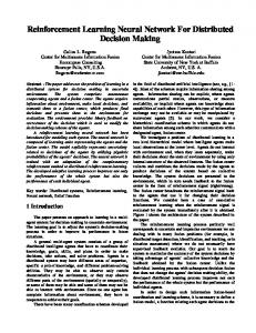
Five years from now on, a 70-nm CMOS process may be available, which is chosen as the future technology for comparison. The gate delay for this technology is not experimentally available. But from the gate delay data from the 2-mm process to 0.35-mm process, it is estimated to be 0.0649ns. It is calculated by using cubic spline interpolation function in Matlab. Given the 31-stage ringer oscillator frequencies in 2.0-, 1.2-, 0.8-, 0.5-, 0.35-µm CMOS processes from MOSIS PARAMETRIC TEST RESULTS, the same oscillator frequency is interpolated to be 497MHz, as shown in Figure 5, then the gate delay of one stage is 0.0649ns.

17

50 0

45 0

40 0

35 0

30 0

25 0

20 0

15 0

10 0

50

0 0

0.2

0.4

0.6

0.8

1

1.2

1.4

1.6

1.8

2

Figure 5: Cubic Spline Interpolation of the 31-stage Ring Oscillator Frequency in 70-nm CMOS Process

Table 7: Time in the 70-nm CMOS process (ns)

Time

1x1

10x10

100x100

1,000x1,000

Serial Digital [9]

2.596

259.6

25,960

2,596,000

Partially Parallel Digital[10]

20.05

200.5

2,005

20,050

Fully Parallel Digital[11]

114.87

114.87

114.87

114.87

Fully Parallel Analog[12]

6.49

6.49

6.49

6.49

18

Table 8: Chip area in the 70-nm CMOS process (mm2)

Area

1x1

10x10

100x100

1,000x1,000

Serial Digital [9]

0.099

0.099

0.099

0.099


0.1027

1.027

10.27

102.7


0.01448

1.448

144.8

14,480


0.00003472

0.003472

0.3472

34.72

Figure 6 is essential the same plot as Figure 4, but with the 70-nm CMOS technology. As shown in the figure, it is possible now to implement 1000x1000 neural network within 1cmx1cm chip area and 1ms computation delay, while it is still not possible to implement with all other methods.

19

1.00E+07 1.00E+06

1.00E+04 1.00E+03

Time (ns)

1.00E+05

1.00E+02

Serial Digital Partially Parallel Digital Fully Parallel Digital Fully Parallel Analog 1x1 10x10 100x100 1000x1000

1.00E+01 1.00E+00 1.E-05 1.E-04 1.E-03 1.E-02 1.E-01 1.E+00 1.E+01 1.E+02 1.E+03 1.E+04 1.E+05

Area (mmxmm)

Figure 6: Area and Time Requirement for Different Implementation Methods with Different Neural Network Sizes for 70-ns CMOS Process

The major drawback of all hardware implementations is that they must often be designed for a specific application. Therefor, their use can be justified only for either very large quantities or very high-performance requirements [13].

General-purpose

digital hardware has an advantage in this perspective. It is available in the market, and only software configurations are needed. In addition, digital hardware is generally easier to design than analog hardware. Analog hardware is more costly to design. However, if the analog design overcomes the design difficulties, and is in mass production, the cost would be much smaller. As mentioned before, neural network controllers can be generalpurpose controllers. Once a good design is ready, it can be reconfigured with minor effort

20

for dissimilar applications.

However, a good analog design that overcomes all the

difficulties is essential. In summary, there are advantages and disadvantages for both digital and analog hardware. When the computation power is not high, it is cost efficient to use software and digital solutions. Only when high computation power is required is the analog circuit preferable, given a good analog implementation. Also, when the power consumption and size is a concern, the analog circuit is definitely preferred.

2.2 Basics of Neural Networks Figure 7 is the model of a single neuron with three inputs and three weights. Every input is connected to the neuron body through a different weight.

Input1 Input2

Input3

Weight1j Outputj Weight2j

Neuron j

Weight3j

Figure 7: A Neuron

The neuron output is a function of its inputs and associated weights, as shown in the following equation:

21

 3  Output j = f  ∑ (Input i * Weight ij ) .  i =1 

Equation 1

The function f ( ) is called the neuron-activation function. A neuron is the basic unit of a neural network. To construct a network, the neurons have to be organized in certain architecture. The following sections present the literature search on all kinds of learning neural network chips, which are compared by chip architecture, learning algorithm, activation function implementation, and synapse implementation.

2.3 Learning Neural Network Chips in Literature When building on-chip learning hardware neural networks, there are three main issues: the chip architecture (the learning algorithm is associated with the chip architecture), the activation function circuit, and the synapse circuit. The first issue is chip architecture, which is determined by the neural network model. The model defines the topology of the neuron connection and associated learning rules. There are three main types of neural network models that have been built in the hardware: the multilayer feed-forward networks, the feedback/recurrent networks, and the unsupervised networks.

22

2.3.1 The Chip Architecture and Associated Learning Algorithms

2.3.1.1 Multilayer Feed-forward Neural Networks The most commonly used neural network architecture is the layered feed-forward topology. As shown in Figure 8, the neuron units are organized in layers. Each neuron within a layer is connected to all the neurons of the next layer. There is no connection between the neurons in the same layer. The inputs to the network are the inputs to the first layer, and the outputs of the first layer are the inputs of the second layer, etc. The outputs of the last layer are the outputs of the network. There are many variations in the layered architecture. Some are not fully connected between layers and the number of layers can vary. However, the type shown in Figure 8 is the most used, which is the twolayer feed-forward fully connected network.

Input Output

Layer1

Layer2

Layer3

Figure 8: The Two-layer Feed-forward Neural Network Architecture

23

The multilayer feed-forward network is usually built by cascading the layers one after another. And each layer is composed of synapses and neurons. The typical chip architecture of one layer of a fully connected neural network is shown in Figure 9. The two dimensional array of synapses ensures that each input has a synapse to each neuron.

Input

Output

Synapse Neurons

Figure 9: The Chip Architecture of One Layer network in a Multilayer Neural Network

The multilayer feed-forwarded structure is associated with the following learning algorithms that are implemented in hardware: back-propagation, contrastive backpropagation, weight perturbation, and random-weight-change algorithms.

24

•

The back-propagation learning In the conventional back-propagation learning algorithm, weights are updated by ∆wij = εδ i o j ,

Equation 2

δ i = ζ i f ' (u i ).

Equation 3

In the output layer,

ζ i = t i − oi .

Equation 4

And in the hidden layer,

ζ i = ∑ w ji δ j , j

Equation 5

25

where ui and oi are the input and output of a neuron i, wij is the weight, f ( ) is the nonlinear activation function, ε is the learning rate, and ti is the target output of the neuron i. •

The contrastive back-propagation learning Offset errors in analog hardware learning circuits give biases to the above

equations. The contrastive back-propagation learning [14] is proposed to cancel either input or output offset errors. In this algorithm, the learning is divided into two phases: clamped and free.

Unlike the conventional back-propagation, it doesn’t use the

difference between the target and the output as the back-propagation error signal. Instead, it uses the target value in the clamped phase and the output value in the free phase. The weight changes for both phases are calculated, then the net weight change is given by the difference of the weight changes for these two phases. This is similar to auto-zeroing. •

Weight perturbation learning rules The back-propagation algorithm assumes linear multipliers. But linear multipliers

are difficult to implement using simple analog circuits. The learning rules introduced here are proposed to be more tolerant with analog nonlinear multipliers. One of the rules is called the serial-weight-perturbation rule [15], or the Madaline Rule III (MRIII).

This algorithm is very tolerant with analog circuit nonidealities;

however, it is a serial computation algorithm. The advantage of the parallel hardware is lost.

26

The chain perturbation rule [16] is based on the serial-weight-perturbation learning rule. The output layer weights are updated directly, following the same learning rule in the serial-weight-perturbation learning rule:

δwkj ∝

∆E , ∆wkj

Equation 6

where δwkj is the change in the weight that connects neuron k to neuron j, and ∆E is the change in error resulting from the perturbation ∆wkj. All weights originated from a given hidden node could be updated in parallel.

Hidden layers are updated by serially

perturbing the hidden node outputs and measuring ∆E/∆o for each hidden node, where ∆o is the change in each hidden node output. Then, hidden weights are perturbed and ∆o/∆w is measured. The weights are updated using the following chain rule:

δwkj ∝

∂E ∆E ∆o . ≈ ∂wkj ∆o ∆wkj

Equation 7

This algorithm is tolerant with nonlinear analog multipliers as MRIII and it is more parallel in learning compared with the MRIII algorithm. However, it is not a fully parallel algorithm either. 27

•

Random-weight-change algorithm This is a gradient descent algorithm like the back-propagation algorithm. The

algorithm [12] can be expressed as follows: W (t + 1) = W (t ) + ∆W (t + 1) ,

Equation 8

If the error at t+1 is decreased compared to that at t, ∆W (t + 1) = ∆W (t ) ,

Equation 9

Otherwise, ∆W (t + 1) = random(t ) ,

Equation 10

where W(t) is the weight at time t and ∆W(t) is the weight change at time t. The random (t) function is either +δ or -δ with equal probabilities. This algorithm implies that when the error is decreased, the weight keeps the direction of the change, otherwise a new direction is randomly chosen. There is an equal probability (if δ is small) of the new ∆W

28

increasing or decreasing the error. There is a detail issue of whether allowing the weight changes that increases the error, which will be discussed further in the future sections. 2.3.1.2 The Hopfield Network and the Boltzmann Machine The Hopfield network is typically used for associative memory applications. A simple example is as follows: The network remembers a clear image (the network gives a certain output for this image), and it is trained to envoke the original image by presenting a noisy version or part of the original image (the network learns to give the same output when the incomplete or noisy image is presented). Generally, the Hopfield network is trained to generate a set of outputs for a set of given inputs. The Hopfield network is a fully connected network. A single change in a neuron would cause changes in all the neurons in the network. After the network has settled, the neuron activation is determined by the following equation:   Vi = f  ∑WijV j  ,   j

Equation 11

where Vj is the current activation of the jth neuron and Wij is the weighting factor that determines the effect the jth neuron had on the ith neuron’s activation. The f ( ) is a sigmoid function.

29

The architecture of a fully connected Hopfield-type network [17] is shown in Figure 10. A network of N neurons has N (N-1) synapse. As shown in the figure, the synaptic circuitry occupies the majority of the chip area.

Synapse

Neurons

Input

Hidden

Output

Figure 10: The Architecture of a Fully Connected Network, with Input, Hidden and Output Neurons [23]

2.3.1.3 The Kohonen Network The Kohonen network is mostly used to classify inputs into different categories, according to the topology relation of the inputs. It has two layers, as shown in Figure 11.

30

The first layer is the input layer; the input patterns are fed through the input layer. The second layer is the Kohonen output layer. It is composed of neurons that compete with each other; each neuron has a positive feedback to itself and negative feedback to others. The chip architecture [18] is shown in Figure 12. The winner-take-all (WTA) matrix is the output layer shown in Figure 11. Neurons in this layer have both the inputs from the input layer and the feedbacks from neurons within the same layer. The WTA matrix is a fully connected network, which has the same architecture as the Hopfield network and the Boltzmann machine shown in Figure 10.

Input Layer

Output Layer

Wij Xi

i

Figure 11: The Kohonen Network

31

j

Yj

Synapse matrix

WTA matrix

.

.

.

.

.

.

.

.

.

Input vector

Output vector

Positive feedback Negative feedback Synapse Output buffer

Figure 12: The One-dimensional Kohonen Network Architecture

The Kohonen learning rule is unsupervised. The weight Wij from the ith neuron in the input layer to the jth neuron in the output layer is modified by the following Kohonen learning rule: ∆Wij = α (X i − Wij )Y j ,

Equation 12 32

where α is the learning rate, Xi is the ith input, and Yj is the jth output. 2.3.1.4 Summary From above discussion, there are three basic types of neural networks. Table 9 compares these three kinds of network architectures. The comparison is made between learning speed, supervised or unsupervised learning, and application areas. Table 9: Comparison of Different Network Models

Network Model

Training Speed

Supervised

Application Areas

Feedback/Recurrent

Very slow

Yes

Associative memory

Unsupervised

Fast

No

Fault detection

Multilayer Feed-forward

Fast - slow

Yes

Most applications

The unsupervised learning model, like the Kohonen model [25], is mostly used for problems where the desired behavior is unknown. The feedback/recurrent model, like the Hopfield model, is generally used for associative memory problems. And the multilayer feed-forward network can be applied on many different applications where the desired behavior is well known. It is the most widely used model today. It is actually a subset of the feedback/recurrent model. Any feed-forward network can be constructed from a feedback/recurrent network. The feedback/recurrent network is thus a more general architecture. However, the training speed is typically very slow and the algorithms are complex. The unsupervised model is the fastest to train. Some of the multilayer feed33

forward networks are fast to train, too, like radial-basis function networks. But they cannot do generalization very well compared with the sigmoid-shaped function networks. 2.3.2 Activation Function Circuit The second issue is the activation function circuit. It is mainly a nonlinear function, which is usually a sigmoid or hyperbolic tangent function. The nonlinear function is usually implemented by an amplifier with the sigmoidshaped transfer function [12] [19] [20] [21] [22] [23] [24] [25] [26]. Usually, the input to a synapse circuit is a voltage, which is then multiplied by the weight. The output of the multiplier is often a current, so that the weight inputs can be summed easily in analog circuits. The activation function takes the sum of current as input and converts the current into a voltage. Thus the chip is cascadable to the next layer. The output of the neuron is usually the input of the neuron on the next layer, which is a voltage. Normally, the activation function is implemented by a sigmoid-shaped transconductance amplifier [12] [27] [28] [20] [29], with a current input and a voltage output.

Some

implementations [22] [23] have a multiplier before the amplifier. The multiplier is used to adjust the slope of the sigmoid function. However, there is a different method [16] [30], which is to implement the nonlinear function as a linear current-to-voltage converter, given that the analog multiplier usually has built-in nonlinearity already. The main difference between this model and the standard model is whether the nonlinearity is applied before the summation or after the summation. The standard model applies the nonlinearity after the 34

summation, while this alternative model applies the nonlinearity on the multiplier, which is before the summation. It is suggested that the standard model is a crude attempt to model a complex biological system, and the important characteristic is the ability to form nonlinear mappings. This alternative method leads to a simpler neuron circuit and saves effort in building the sigmoid or the hyperbolic tangent curve. In other cases [25] [31], the neuron activation function is a high gain sigmoid function, called threshold function. When the sum of the current is larger than the threshold, the neuron output is high; otherwise, the neuron output is low. For this purpose, a comparator is needed. For the Kohonen network [25], the output layer is a winner-take-all network. The output value is either high or low, and only one output neuron is high. Therefore, a buffer is used for the output. 2.3.3 Synapse Circuits The major challenge in analog VLSI implementation of neural networks is synapse circuits (the weight storage, modification, multiplication). Much research has been done in this area [32] [33] [34] [35] [36] [37]. But until the early '90s, there is no weight adaptation hardware built on chips, the learning is performed on computers, and then the weights are hard copied onto the chip. Ideally, the weight is to be held in a longterm storage, and it should be modified easily [38] [39]. In reality, the permanence of the stored weight had to be traded against the ease of its modification.

35

There are five kinds of weight circuits, categorized by storage type. They are the capacitor-only weight, the EEPROM weight, the capacitor with refreshment weight, the digital weight, and the mixed digital/analog weight. 2.3.3.1 Capacitor-only Weights Several researchers [12] [21] [22] [23] [25], use only a capacitor as the weight storage. Since the circuits are built for different applications, the learning algorithms and the chip architectures differ. However, the basic synaptic circuits are similar. The circuits in publications [12] [21] [23] use the Gilbert multiplier, the four quadrant Gilbert multiplier, and the transconductance multiplier, respectively.

The

weight is stored on a capacitor and adjusted by a current Ic, as shown in Figure 13.

Yp XP M2 Ic

XN

Vw

M1 Cw Yn

Figure 13: The Weight Storage and Modification Circuit [23]

In the figure, Yp and Yn are connected to the positive and negative voltage sources. The voltage Vw across the capacitor Cw represents the weight. Pulse signals XN and XP

36

added to the gates of M1 and M2 decrease or increase the voltage across Cw, thus modifying the weight. The weight changes are governed by dVw I = c . dt Cw

Equation 13

The main problem with the capacitor-type circuit is that the current leakage causes the weight to drift. In circuits [23] [21], the leakage current is less than 1pA. To reduce the leakage current, the chips can be cooled in a slightly lower temperature. If the chip is used under the condition where the weights are updated fast enough, the leakage current can be ignored. Continuous learning process also provides a way for the network to compensate for component drift as the temperature of the circuit changes. Figure 14 shows another weight storage and the update circuit [22], which is similar to the one shown in Figure 13. The multiplier used in this implementation is also the Gilbert multiplier.

37

Yp

XP

M2

C2 -

XN

M1 + C1 Yn


The weight-modifying signal is a voltage; after a voltage-to-pulse converter, pulse signals XN and XP are added to the gates of M1 and M2. As in the previous figure, Yp and Yn are connected to the positive and negative voltage sources. The weight value is stored in capacitor C1. To minimize the nonlinearity caused by the change in the capacitor node potential XC during the learning operation, a feedback path including the op-amp and the capacitor C2 is added. The charge stored in capacitor C1 is then transferred to the capacitor C2. The capacitance of C1 and C2 is 20 pF. In this circuit, the weight decays by itself because the charge stored in the capacitor leaked through the junctions: the p+n junction of the PMOSFECT M2 and the n+p junction of the NMOSFET M1. At room temperature, the leakage current at the p+n junction is larger than that at the n+p junction [22]. The weight usually decreases as time passes. The time constant of the decay is about 104 sec, which is fairly large compared with the typical retention time in dynamic RAM’s. The reasons for such long retention time are as follows: (1) the very large capacitance (20pF), (2) the small junction area 38

resulting from a double poly process, and (3) the compensation between the two leakage currents through the two complementary junctions. As a result, a 13-bit precision is maintained for 1s, and 10-bit precision is maintained for 10 s. The retention time is considered long enough to use the chip in the applications where weights are always updated. This synaptic chip is fabricated in 1.3-µm CMOS, double metal, and double poly process. The 7mm x 7mm chip consisted of nine neurons and 81 synapses. For the network [25] that has one bit input to each input neuron, the multiplier is not necessary. But the weight storage and modification circuits are shown in Figure 15.

φ1

φ2

Input X Cw

C1


The Cw is the weight capacitor, the C1 is the parasitic capacitance, and φ1 and φ2 are two nonoverlapping clocks. When the φ1 goes high, the capacitor C1 is charged to the input voltage X; the charge on C1 at the time is Q1=X(t)C1. When φ2 goes high, the charge in both capacitor C1 and Cw is redistributed. Assuming that the initial voltage across Cw is W(t), the charge stored at Cw is Qw=W(t)Cw. According to the charge

39

conservation law, the charge must be constant before and after the charge sharing. The final voltage across both capacitors is

W (t + 1) = W (t ) +

C1 ( X ( t ) − W (t ) ) . C1 + C w

Equation 14

Since Cw>>C1, the new weight voltage is

W (t + 1) = W (t ) +

C1 X (t ) . Cw

Equation 15

Thus, every time, the weight is modified proportionally to the input signal X. The test chip is fabricated with 2-µm CMOS technology. The chip size is 2.2 mm x 2.2mm. The network actually takes an area of 0.9mm2, including 120 synapses. The weight storage capacitor Cw is 1.18pF, with an area of 38µm x 38µm. The leakage source is a p-n junction of 6µm x 6µm in size. The leakage is negligible at room temprature when the clock frequency is above a few hundred kilohertz [25]. The implementation in the publication [12] uses a similar charge-sharing scheme to modify the weight with a simpler multiplier. transistors, as shown in Figure 16. 40

The multiplier consists of three

Yp In Vbias Out = in * Vw Vw Cw Yn

Figure 16: The Weight Storage Circuit and the Multiplier Circuit [12]

The chip (2.2mm x 2.2mm) is built in a 2-µm CMOS double poly process, including 100 weights. The 2pF capacitor is built by double poly and the current leakage on it caused 10% loss of the weight value in 5s. Generally, the chip using the capacitor as the weight storage takes a very small area. The weight modification is either by current or by charge sharing. The multiplier most used is the Gilbert multiplier. Capacitor-type weight storage provides the network with a dynamic, easy-to-modify memory, thus enabling the circuit to learn on-chip. However, the drawback is that the current leakage on the capacitor caused the weight to drift. The capacitor needs to be fairly large to hold the voltage. It ranges from 1pF to 20pF, which takes about one third of the synapse area [12]. For a system that is constantly changing, the weight updating may be fast enough to compensate for the leakage. Cooling process can also reduce the current leakage significantly. However if the results of learning are to be restored after the power is

41

removed or the learning pattern is remembered or if the pattern to be learned is long in time, nonvolatile memory is essential to save the learned information. 2.3.3.2 EEPROM Weights The EEPROM is a nonvolatile memory in the analog process. It is good for longterm memory storage. However, the weight modification is not easy to implement. Early works in EEPROM hardware [40] [41] had no learning ability. The circuit in publication [16] uses a combination of dynamic and nonvolatile memory that allows both fast learning and reliable long-term storage. The schematic of the synapse circuit is shown in Figure 17.

I+

I-

I+

Yp

V+

V+

M2

Vcgref F2 Cpert

M1 Yn

I-

V-

F1

Chold

Vpert

Vdss

Figure 17: The Schematic of the Synapse Circuit [16]

In Figure 17, M1, M2, and Chold form a dynamic memory. The capacitor Cpert is for perturbation as required for the perturbation learning rule. And the reminder is a

42

modified Gilbert multiplier with floating-gate device current sources, as in the ETANN chip [41]. First, changing the voltage on the Vpert line perturbes the weight; transistors M1 and M2 are turned off. The weight voltage stored on Chold is perturbed by the amount proportional to the change of Vpert. Then, using the learning rule, an error is calculated. The control circuit for the weight adaptation determines either to turn M1 on to decrease the weight or to turn M2 on to increase the weight. As the Vpert returns to its original value, the weight remains the same as before the perturbation. So, the weight is increased or decreased from the point before perturbation. The modified Gilbert multiplier implements the feed-forward multiplication. The differential output current is

I+ − I− =

4 I F1 K  4 I F2 Vin − Vin2 − − Vin2 2  K K 

 ,  

Equation 16

where Vin is V+-V-, K=µ0Cox W/L and IFi is the current of the floating-gate device i. The 64-synapse, eight-neuron chip is fabricated using the Orbit Semiconductor’s 2-µm, double poly, and double metal technology, with a chip area of 2.2 x 2.2 mm2. It includes the features of on-chip learning, but without the ability to program the floating-

43

fate memory. The floating gates are programmed using hot-electron injection after the learning is complete. Even though the nonvolatile memory is present, it is hard to change on-line. Instead, the nonvolatile memory has to be programmed after the learning is complete. This limited the areas in which this chip can be used. For example, in the area of nonlinear adaptive control or the engine combustion stability control, the system is continuously changing with the time, which requires the neuron network to adapt continuously on-line. Also, in other applications, the chip may not be accessible to program once it is put into use. 2.3.3.3 Capacitor with Refreshment Weights There are two methods for the weight refreshment. In the first method, a static RAM followed by a D/A converter refreshes the weight stored on a capacitor. Two chips are fabricated using this method. In the first chip [24], the unit synapse size is 33280 µm2 with 10-bit resolution. The second 1.6mm x 2.4mm chip [20] contains 18 neurons and 161 synapses, fabricated in 3-µm CMOS technology. The resulting unit synapse is 3564 µm2 (54 µm x 66 µm). In the second method [42], the weight-refreshing scheme is based on an A/D conversion followed by a D/A conversion of the weight value. Periodically, each weight voltage is read and transferred through the A/D and D/A converters, the discrete version of the weight value is then written back to the weight storage capacitor. The seven-bit

44

resolution A/D and D/A converters are implemented once per chip, and the weights in a chip are refreshed sequentially. The network with on-chip Hebbian learning and weight refreshing is fabricated in a 2-µm, double poly standard CMOS process (MOSIS). It contains 25 synapses and a pair of A/D and D/A converters. The shortcoming of the weight-refreshing scheme is that the weight is limited to certain discrete values. The resolution of the A/D and D/A converter limits the resolution of the learning weight. Usually, a 15- or 16-bit resolution is needed for learning. To build a 15- or 16-bit A/D and D/A converter is space consuming and expensive. In the second method, it is good that the A/D and D/A are only implemented once per chip. However, the weights then have to be refreshed sequentially one after another. Since the time interval to refresh one weight is fixed for a certain size of capacitor, this refreshing scheme limits the number of weights that can be built per chip. Also, the sequential refreshing scheme is not a fully parallel operation of the weights. 2.3.3.4 On-chip Digital Weights Two methods are used for the on-chip digital synapse. The first method [19] is shown in Figure 18. The weight is an eight-bit static RAM. The analog learning signal is transferred to a digital signal by a one-bit A/D converter.

This one-bit digital signal is used to modify the weight.

To realize

multiplication using an analog multiplier, the digital weight is transferred to an analog signal by an eight-bit D/A converter. 45

The synapse chip is fabricated in a 0.8-µm CMOS, double metal, and single-poly process. The 6.8mm x 6.8mm chip includes 576 synapses. The actual synapse size is around 200µm x 200µm [19].

Analog Multiplier In

Out

8 bit D/A Weight 1 bit A/D Learning Signal

Figure 18: Synapse Weight Update Scheme [19]

In the second method [43], the synapse is implemented using an analog multiplier too, but with a multiplying D/A converter (MDAC). The synapse circuit with a multiplier and a 4-bit connection weight is shown in Figure 19. The MOSFETs controlled by the bias voltages have binary-weighted width-to-length (W/L) ratios.

46

I1

I2

V+

B1

V-

B2

B3

B4

Vbias

Figure 19: Multiplier Circuit with 4-bit Connection Weight [43]

The synapse and neuron chips are fabricated in a 3-µm technology. The chip size is 2mm x 3mm, including seven neurons and 49 synapses with six-bit resolution. The estimated synapse size is around 250µm x 250 µm. Compared with the previous chip, this one has six-bit resolution instead of eight-bit, and the fabricating process is three times bigger in minimum size. This chip is estimated to take a smaller area given the same resolution and the same process. The synapse areas of the two chips are acceptable. But, it is shown that at least 15 or 16 bits of accuracy is needed in learning by most learning algorithms [20]. The two chips here don’t reach the resolution. The D/A and A/D converters in the method also needs to be extended from eight bits to 15 or 16 bits, which is hard to implement using simple circuits, and will take even more area. This will make the chip more expensive than that with the analog type memory. 47

2.3.3.5 Mixed Digital/Analog Weights The mixed digital/analog synapse circuit is introduced in the publication [44]. The digital part of the weight is shown in Figure 20, which is similar to that in the second method introduced in the previous section.

-1 ½ ¼ Isk B-1

1/2 Wkj0

Wkj1

Wkj2

WkjB-1

Vss

gm

vzj

Vss

Figure 20: Digital Storage for Digital/analog Hybrid Synapse [44]

The transconductor gm and the diode coupled transistor transforms the input voltage vzj to a current. The voltage is applied to the gates of the transistors at the synapse sites and causes proportional drain current gmvzj. The multiplication is performed by switching the current sources to or from the horizontal current accumulation lines,

48

controlled by the locally stored synapse strength word. The currents are then binary weighted and summed. The current output from a row of synapse is given by M M B −1 1 M bb 1 bb   b0 w g v g w w v g = = − +   ∑ zj m ∑ wkj vzj , m∑ kj kj b ∑ kj m zj b j =1 b =1 2 j =1 j =1  b =1 2 

B −1

M

isk = −∑ wkj0 g m vzj + ∑ j =1

Equation 17

where wkjbb is the bth bit of the weight wkj (stored as a two’s complement signed number), B is the number of bits in wkj, and M is the number of row inputs. The authors of the paper proposed to combine the digital memory with a simple capacitor for the accumulation of small weight changes. Thus, the simple analog circuit can handle the weight change, and the hardware cost of the learning algorithm is minimized. The proposed analog extension is shown in Figure 21.

Analog Extension

VAE+ VAEkj Up

Counter Down Vss Reset VAE-

Figure 21: Analog Extension of a Mixed Analog/digital Weight [44]

49

Digital weight

The analog extension voltage VAEkj is changed by a current output multiplier, which is part of the learning algorithm hardware. When the voltage VAEkj is outside the range of [VAE-, VAE+], the corresponding digital weight is increased/decreased accordingly by the up/down counter. At the same time, the analog extension voltage is reset to zero. The analog capacitor weight enables the network to do on-chip learning easily, with simple and compact analog circuits. The digital weight provides the nonvolatile memory. Compared with the combination of capacitor and floating-gate weight, the digital weight is easier to modify on-line than the floating-gate device. 2.3.3.6 Summary Table 2 compares these five types of synapse circuits. The comparison is based on unit synapse area, resolution of the weight, the need for off-chip memory, the ease of modification, and nonvolatile memory. The area is for one synapse circuit, in the unit of 1Kµm2. They are normalized to a 1-µm process. For example, if a synapse takes 200µm x 200µm area in a 2-µm process, it is normalized 100µm x 100µm = 10000µm2 in a 1-µm process. The ideal chip should have a relatively small synapse area. The weight resolution is for the digital related weights. The on-chip digital weights has the resolution of its own; the capacitor-withrefreshment weights are limited by the resolution of the off-chip digital memory or the A/D and the D/A converters. The capacitor-based memory is an analog signal and is supposed to have infinite resolution. None of the networks need off-chip memory, except for the chip that is built with off-chip refreshment. 50

Table 10: Comparison of Five Kinds of Weight Storage Circuits

Storage type

Area

Resolution

Off-chip

Modification

Nonvolatile

memory Capacitor-

1.3 (1.18pF)

only

5.6 (2pF)

Analog

No

Easy

No

Analog

No

Easy/hardest

Yes

7, 8, 10b

Yes

Easy/harder

Yes

131 (20pF) EEPROM

1.2

Capacitor w/ 0.8 (0.32pF) Refreshment Digital

6.25/125

8b

No

Fair

Yes

Mixed D & A

?

Analog

No

Fair/easy

Yes

The digital weights shown here have eight-bit resolution.

According to the

author, the synapse area is not big, normalized to 6.25 Kµm2. However, to make the circuit function, some peripheral circuits are needed.

The 6.8mm x 6.8mm chip

fabricated with 0.8-µm process contains 576 synapses, which resulted in a normalized area of 125 Kµm2. It has been shown [20] that 15- or 16-bit resolution is needed for learning, and five- to eight-bit resolution is needed for storage after the network has been trained for a while. Therefore, the eight-bit resolution is good enough for storage, but

51

may not be enough for learning. To reach the required resolution for learning, it will take too much area for the digital weight circuit. Although the EEPROM weight is a very compact and nonvolatile memory, it is process sensitive.

Usually, extra compensation circuits are required to solve this

problem. The capacitor with refreshment weight needs off-chip memory, which is not a compact solution.

The additional A/D and D/A required make the chip more

cumbersome or resulted in serial operations. Capacitor-only weights are compact and easy to modify. However, they have the problem of leakage.

To prevent leakage, the capacitors are made very big (20pF),

resulting a size around the same an eight-bit digital weight. However, for the applications where leakage is not a problem, the capacitor-only weight is a good solution. The mixed digital/analog-type weight storage is a balanced solution when nonvolatile memory is necessary. The theory behind this is that although about 15-bit resolution is needed for learning, only about eight-bit resolution is needed for storage. Therefore, a weight with eight-bit digital memory together with an analog capacitor weight is preferable. The digital circuit thus provides nonvolatile memory, without too much area. The capacitor circuit has the advantage of easy modification and provides enough resolution for learning. However, no one has yet researched this experimentally.

52

2.4 Application Areas of Learning Neural Network Chips in Literature Most of the neural network chips with the multilayer feed-forward architecture are usually tested with the two-input XOR problem [12] [22]. This is a static problem, where the four possible input combinations are fed to the network, and the corresponding network output is compared with the desired output, thus providing an error.

The

learning algorithm then changes the weights accordingly to minimize the error. The four combinations are fed to the network again, and the error is calculated accordingly; the weights are then changed to decrease the error. This process goes on until the error is within some limited tolerance. Thus, the network is trained to implement a two-input XOR logic; that is, the output is the result of the XOR logic performed on the inputs. The input and output relationship is static and does not vary with time. Because the XOR problem needs two layers of feed-forward network to solve, it is assumed that it is a good measurement of the learning ability of the neural network. However, there is envidence that the XOR problem is not very similar to many practical problems Another application area is the sine wave identity-mapping problem [19], which is also a static mapping problem.

The pattern recognition or association applications

usually have their own special architectures, like the Kohonen network and the Hopfield network, and are beyond the control application area discussed here. There are no learning neural network chips fabricated for real-time control applications in the literature. Most of applications use software neural networks running

53

on a computer, which output a control signal to the plant through some digital or analog output cards.

54

CHAPTER III

REAL-TIME CONTROL WITH HARDWARE NEURAL NETWORK

3.1 Real-time Control Scheme A general direct feedback scheme [45], as depicted in Figure 22, is proposed for real-time nonlinear system control, using learning neural network chips.

Control signal

Output

Tapped Delay Line

Plant

ANN Controller

Figure 22: A Neural Network Controller

In static systems, their inputs and outputs are uniquely mapped. However, the outputs of dynamic nonlinear systems depend on internal states, system parameters, and 55

inputs. Moreover, for nonlinear systems, their system parameters vary with the time and operating conditions. In Figure 22, the tapped delay line is used to sample the plant output history; it should be long enough for the neural network to infer the state of the plant. In general, a period of the plant output of the slowest signal frequency is to be covered. At the same time, the tap delay line should be faster than the Nyquist sample frequency of the highest signal frequency.

The rule is that the neural network should be provided enough

information about the plant dynamics.

3.2 Application of Neural Networks for Real-time Control A neural network controller is desirable only when the plant model is not complete, or is too complicated to determine and no proof of controller stability is required. If the plant is a linear system, a very good controller can be computed from the plant model, which can yield much better performance. If the plant is well understood, a nonlinear controller might be designed to provide provable stable control too. However, for the plant whose the model is poorly understood, or likely to change dynamically over time, neural networks might provide a good sub-optimal solution, though no proof of stability can be provided in the neural network control. Most of the neural network learning algorithms described in the literature have not been proved to yield stable control. In the case of the RWC algorithm, a true random number sequence can produce sufficient long ones or zeros, which could make the learning algorithm fail.

56

However, the chance of this happening is probably lower than the chance of combustion hardware failure.

3.3 Issues for Hardware Neural Networks 3.3.1 The Chip Architecture From the review in the previous sections, the feed-forward architecture is chosen. Since most industrial control applications need some desired outputs, supervised learning is required. In addition, considering the need for generalization, the multilayer feedforward model with sigmoid-shaped nonlinearity is the most suitable model for real-time control applications. 3.3.2 The Learning Algorithm The most well-known algorithm associated with this type of architecture is the back-propagation algorithm. However, it is very sensitive to uncertainty. It requires precise implementation of the mathematical units, like adders, multipliers, and derivative units. It is not a hardwarefriendly learning algorithm for analog circuit implementation. Also, the architecture that uses the back-propagation algorithm in feedback control is very complicated. It cannot be used directly in the proposed control scheme. As shown in Figure 22, the output of the controlling plant is usually fed to the input of the neural network, and the output of the neural network is the control signal that

57

controls the plant. For a given plant output, i.e., a given neural network input, the desired neural network output is needed for the back-propagation algorithm to train the neural network. However, this is the control signal that needed to be generated by the controller, which is unknown and to be found. Thus, the back-propagation algorithm is not suitable for this type of real-time control. There are other algorithms, like the serial weight perturbation [46] (or Madaline Rule III) and the chain perturbation rule [16] that are implemented with hardware circuits. But none of them is a fully parallel learning algorithm, which means the time cycles required for all the weights to be updated once increases proportionally to the network size. The RWC algorithm is more suitable for industrial control applications. According to the learning rule, the weights are changed in a direction to minimize the error. The error is not specified as the network output (difference between actual output of the network and the desired output); instead, it can be any error. For the control problem, the error can be at the plant output (difference between the actual plant output and the desired plant output). 3.3.3 The Activation Function Circuit As explained in Section 0, the current to voltage converter is used as the activation function circuit, since the analog weights includes the nonlinearity already.

58

3.3.4 Synapse Circuit. The original RWC chip [12] used capacitors as the weight storage unit. Potentially, there would be the leakage issue, and a nonvolatile weight is desirable. However, for this research, the controlling plant is a dynamic system, which changes fast with time. The author hoped that the weights would continue to adjust on-line, so that the leakage could be compensated. However, no conclusion was drawn before actually applying the chip for control. It is the goal of this research to address this leakage issue, among other issues, like the multiplier nonlinearity, the learning algorithm implementation, and the learning step etc. Before this research, the RWC chip was tested and proved functional with off-line batch mode learning to implement the two-input XOR [12]. The main purpose of this research is to apply the RWC algorithm and the existing chip to the real-time control domain. The goal is to find the main issues that are critical to the real-time control applications, to make appropriate modifications to the chip, and to provide a new, effective scheme for the real-time control with neural network chips.

59

CHAPTER IV

EFFECTS OF ANALOG CIRCUIT NONIDEALITY As described above, analog circuit implementations of neural networks has nonlinearity in multipliers. To ensure that the RWC learning algorithm is tolerant of the multiplier nonlinearity, a software simulation is performed using RWC algorithm, with nonlinear multipliers. The results shows that the RWC algorithm has successfully trained the neural network to perform on-line control for an induction motor to generate the desired the stator current, despite the analog circuit nonidealities.

4.1 The Induction Motor Application The induction motor is a complex, multivariable nonlinear dynamic electromechanical system. The objective of induction motor control is to control the flow of power into the motor, so as to produce a torque on the rotor shaft, which would result in a desired shaft speed.

To produce the desired torque, the stator current is first

calculated. Based on the required stator current, the applied voltage is then calculated. The relationship among the applied voltage, resultant current, torque, and speed is shown in Figure 23.

60

Voltage

Current

Torque

Speed

Figure 23: Relationship between the Stator Voltage, Current, Shaft Torque and Speed

The relationship between the applied stator voltage and the resultant stator current vector is nonlinear with respect to the speed of the motor shaft. This relationship is also implicitly time varying because of electrical parameter variations. For example, the inductance can vary significantly and rapidly because of significant and rapid changes in current magnitudes; the AC resistance of conductors is frequency dependent and can vary rapidly with rapid changes in current frequency and the relatively slow changes in resistance resulting from the heating effect. In addition, the relationship between the stator current and the mechanical torque is also nonlinear and affected by time-varying parameters. The shaft speed is determined by the net torque applied and the mechanical load. Therefore, the dynamic performance of the motor depended on how well the controller could adapt to the parameter variations.

The two-layer neural network

controller developed by Burton et al. [47] successfully controlled the induction motor to produce the desired current, using a modified version of the RWC algorithm. The modified algorithm makes 20 random trials to change the weight in 20 different directions and calculates the error for each trial. One trial is in the direction of the previous round. However, each change is not permanent. The permanent change is

61

made in the direction of the trial with the least error. The underlying idea is the same as the algorithm explained in the previous section. The modified version improves the algorithm by making more trials, but taking a longer time for each trial. The simulation of the neural network in [47] was based on ideal multipliers and did not include any nonidealities of the analog circuit. One result of using the RWC algorithm in that work is shown in Figure 24. The horizontal axis is time in seconds, and the vertical axis is the current. The dotted line is the desired current, and the solid line is the actual current generated. An ideal multiplier was used in the simulation. In less than 0.1 second, the neural network learned to follow the desired current output. In this case, the simulation was carried out with ideal two-sided multipliers. In the next section, the performance of the neural network with nonideal one-sided multipliers is shown.

62

Figure 24: Simulation Result of Induction Motor Using the RWC Algorithm

4.2 Analog Circuit Nonideality and Simulation Result Based on the fabricated circuit in publication [12], the neural network controller was tested for the induction motor with one-sided nonlinear multipliers. A multiplier can be expressed as y = w x f(x). An ideal multiplier is linear and two-sided, which means x can be positive or negative, and f(x)=1. However, for the nonlinear and one-sided multiplier, as implemented by the analog circuits in [12], x can only be positive, and f(x) is a nonlinear function of x. The ideal multiplier and the nonlinear, one-sided multiplier are shown in Figure 25. The nonideal multiplier shown is

63

an example, and it is defined by y = w * x * (1-x2/3). The dotted line characterizes the ideal two-sided multiplier, and the solid line is the nonideal multiplier. When a multiplier is implemented with an analog circuit, it not only has nonlinearity, but also offset, as shown in Figure 26, which is the measured data from the RWC chip [48]. Substituting the ideal multiplier with the nonideal multiplier in Figure 26, the performance of the neural network controller stated in the previous section was simulated. The result of the generated current is shown as the solid curve in Figure 27. The dotted curve is the generated current using an ideal multiplier. It is the same current as shown in Figure 24 and is redrawn here for comparison.

Ideal Multiplier and One-sided Non-ideal Multiplier

y

x

Figure 25: Ideal Multiplier and the One-sided Nonlinear Multiplier.

64

Figure 26: Multiplier Measured from the RWC Chip

65

Motor Current

Comparison of Control Result with Ideal and Non-ideal Multipliers

with ideal multiply with non-ideal multiply

Time (second)

Figure 27: Simulation Results of Ideal Multipliers and Nonideal Multipliers

The previous work using ideal multiplier was simulated with Matlab software. The nonlinear multiplier operation was very slow when formed from the measured result using the curve-fitting function provided by Matlab. In this case, it was actually so slow and performed so much computation that no result is generated from the program. C program was written for a simplified curve-fitting function and an interface program between the C code and the Matlab code was written. It helped to improve the running speed.

The C code is compilable, while the Matlab code is line executable. This

difference makes C code faster to run, especially for loop functions, which were heavily used in this computation. The C code for curve fitting and the interface code to Matlab are shown in Appendix A.1 Nonlinear Multiplier Simulation Code; it includes the measured data points of the nonlinear multiplier from the RWC chip.

66

The result shown above proved that the RWC algorithm is immune to the analog circuit nonidealities.

67

CHAPTER V

COMBUSTION INSTABILITY PROBLEMS The combustors used in propulsion and industrial applications are by nature unstable.

They have randomly appearing oscillation with different frequencies and

damping. The instability occurs when the combustion process couples with the acoustic field in a way that excites one or more natural acoustic modes in the system [49]. The following passive approaches for eliminating such instabilities are [50] well-known. (1) To modify the combustion process to reduce the magnitude and/or change the frequency dependence of its driving; (2) To increase the combustor's damping; (3) To prevent the excitation of unstable combustor modes; and (4) To shift the frequencies of a combustor's unstable modes away from the range where the combustion process driving is maximized. Unfortunately, these approaches are costly and time consuming. They sacrifice the combustor's performance for stability. Nevertheless, they often fail to adequately damp the instability. Consequently, interest in developing active control systems (ACS) for damping such instabilities has increased in recent years.

68

Efforts to do this started with theoretical considerations in the 1950s (see paper [50] reference [2-4]), and are followed by the eventual demonstration of the feasibility of such control in the 1980s (see paper [50] reference [5-15]). A typical actively controlled combustor consist of a combustion chamber, a sensor, an observer, and the actuator. The sensor detects the instability, the observer determines the state of the system, the controller modifies the observer's output to provide a signal to an actuator, and the actuator perturbs the systems in a controlled manner. Ideally, ACS can be effectively used in different systems, with operating conditions that change with time. In addition, it would be suitable for systems whose behavior is not fully understood. The ACS approach is significantly less expensive and more dependable than the passive approaches. Previously reported ACS were designed to damp instabilities consisting one or two modes (see paper [50] reference [14]) whose characteristics were generally assumed in advance. Later, adaptive control system (see paper [50] reference [12]) were proposed that used an iterative scheme to optimize the controller parameters that stabilize a specific mode. The performance of this controller, after a relatively long adaptation time, proved superior to that exhibited by the fixed-parameter controller.

However, it also, on

occasion, destabilized stable system modes. Moreover, since real combustors exhibites sudden changes in the active modes, such a controller, with its parameters optimized for a specific frequency, may actually amplify the oscillations when the frequency of an unstable mode changes.

69

To effectively suppress combustor pressure oscillations, an ACS must absorb energy from the system at the frequencies of the unstable modes. Rayleigh's criterion [51] states that the performance of an ACS is optimized when the energy added to the system is out of phase by a half cycle relative to the local pressure oscillations. Such a strategy can be easily implemented with an ideal actuator with no time delay between the input signal and the energy addition process.

However, ideal actuators that can

instantaneously and accurately respond to input signals do not exist. Compensatory unit is added to the control system to account for the actuator dynamics, if the actuator dynamics could be modeled. However, the fuel injector actuators used for controlling combustion instability have highly complex dynamics, which are not known and cannot be modeled. Neural networks have the ability to deal with unexpected or new things when used on a real plant. They are superior to the traditional control methods when a plant model cannot be easily expressed by a math equation. They continuously adjust their weights to give a relatively optimized control signal to reach the goal, in this case, to stabilize the engine. The following steps were carried out to control combustion instability with learning hardware neural networks. 1. Software simulation: Extensive software simulations were carried out on the neural network control of combustion instability. combustion instability were tested. 70

In the simulations, two models of the Experienced combustion researchers

suggested the models. The two models were undamped oscillators and limit cycle oscillators. The result showed that the combustion could be stabilized under the neural network control. 2. Preliminary hardware modifications and tests: After being assured by the software simulation, the RWC chip was redesigned and tested. The modifications were to make the RWC chip more suitable for real-time control applications. The original chip was designed for static problems and tested on digital applications. The presented problem was a nonlinear, dynamic problems that required analog input and weight ranges. The hardware tests were intended to verify the basic functions of the designed neural network, for example, the possible defect in the chip in the fabrication process, the appropriate data range when coordinated with the computer and the data acquisition cards, and how well the chip implemented the learning algorithm. 3. Hardware chip controlling computer simulated plant: This was a closed-loop test on combustion instability control, with the hardware chip, computer-simulated combustion instability model on PC, and data acquisition cards in between. The following three chapters are devoted to the above procedures.

71

CHAPTER VI

SOFTWARE SIMULATION OF COMBUSTION INSTABILITY CONTROL

6.1 Introduction The basic simulation setup is shown in Figure 28. The pressure of the unstable combustion engine is detected as the engine output x. It goes through a tap delay line, where it is delayed and stored. A series of the engine outputs is then fed to the neural network controller. The neural network adjusts its weights and generates a control signal to stabilize the engine. After a delay, the control signal is fed to the engine as engine input u. The delay represents the actuation delay of the engine. The error is generated by envelope detection of the engine output.

72

x Unstable Combustion Engine

error

error

Delay line

Delay 1.5 ms

u

Software Simulation of Neural Network Chip Figure 28: The Neural Network Control of Unstable Combustion Engine System

In the software simulation, the engine was represented by differential equations, which were solved using Runge-Kutta method with a step size of 1/80,000 second. The neural network was simulated with the same learning algorithm that was actually implemented by the existing hardware neural network chip. The software engine simulation went through the following stages, defined by the complexity of the engine model and the model parameters. •

Undamped oscillator-one fixed frequency with changing damping factor

•

Undamped oscillator-two fixed frequencies with changing damping factor

73

•

Limit cycle oscillator-one fixed frequency with changing damping factor and different limit cycle constant

•

Limit cycle oscillator with continuously changing plant parameters-frequency, damping factor, and limit cycle constant.

•

Limit cycle oscillator with added noise at engine output.

The simulation results of each stage are presented and explained in the following sections.

6.2 Undamped Oscillatory Plant 6.2.1 Single Frequency Using the control strategy in Figure 28, a simple combustion model was first tested. It assumed that the plant had a single unknown unstable oscillatory mode. The plant model is expressed by the following equation: !x! − 2ζωx! + ω 2 x = u ,

Equation 18

where, x is the engine pressure output, and u is the engine input.

The oscillation

frequency ω was 400 Hz. The damping factor ζ was in the range of [-0.005, 0.0). The damping factor in this range made the plant unstable and oscillate to infinity with different speed. The combustion control signal was delayed by 0.6 times the combustion 74

oscillation period of 400 Hz. The tap delay line had eight taps, covering a total of 2.5 milliseconds. The neural network has two layers. The first layer had eight input neurons, one hidden neuron with fixed weight, and one output neuron. The learning rule allowed the weight changes that increased the error. The error detection was magnitude. The neural network seeks to drive the combustion model output to zero. The source code for the simulations are in Appendix B.1 Unbounded Oscillator-One Frequency. Figure 29 presents the simulated response of the hardware neural network controlled combustion.

Starting with an untrained network, the ζ parameter of the

combustion model had the values in Table 11, which was a pseudo-random change in oscillation stability.

After the network had run for a while, the time to converge

decreased significantly for a given ζ. Every 5 seconds, the engine was re-assigned a starting state, with the engine pressure to be 0.5, and the damping factor ζ randomly chosen. Table 11 lists the ζ values used at each time the combustion was reinitialized. The neural network, however, was NOT reset when the engine was. So, the neural network remembered the weights learned during the past periods. As time went by, the neural network gradually learned more and performed better and better. This was evident by the time it needed to stabilize the oscillations with the same damping factor. For comparison, Figure 30 shows the combustion instability without the control, with the same set of damping factors in Table 11. They all oscillated to a magnitude of 1000 in less then 5 seconds, at different speed. Figure 31 is the same as Figure 29, with the weight change shown.

75

Table 11: The ζ Values

ζ -0.001 -0.004 -0.002 -0.003 -0.004 -0.002 -0.001 -0.003 -0.002 -0.003 -0.004 -0.003 -0.005 -0.001 -0.005 -0.004

Time 0 5 10 15 20 25 30 35 40 45 50 55 60 65 70 75

76

Figure 29: The Results of the Simulated Hardware Neural Network Controller

77

Figure 30: Combustion Model without the Neural Network Control

78

4

2

3

4

2

1

3

2

3

4

3

5

1

5

4

NN Weight

Engine Pressure

−1000ζ= 1

Time (second)

Figure 31: Redraw of Figure 29, with the Damping Factor and the Weight Values

6.2.2 Multifrequency After the one-frequency simulation, the combustion was then modeled with two fixed frequencies, with changing damping factors. The setup and simulation procedure were similar to the one-frequency case.

The plant was modeled by the following

equation: 2 x!!k − 2ζ k ω k x! k + ω k x k = u ,

Equation 19

where k=1,2, u is the engine input, x=x1+x2 is the engine output. The first oscillating frequency was 400Hz, the second oscillating frequency was 700 Hz. And the damping 79

factors ζ1 and ζ2 were in the range of [-0.002, 0.0]. As before, the damping factors made the plant oscillate to infinity. The actuation delay was modeled as 0.6 times the lowest frequency, 400 Hz, which was 1.5 milliseconds. The tapped delay line had 12 taps, which covered 3.75 milliseconds in time. The neural network had 12 input neurons, two hidden neurons, and one output neuron. The learning rule allowed weight changes that increased the error. The error was obtained by envelope detection of the engine output. The source code for the simulation is shown in Appendix B.2 Unbounded Oscillator-Two Frequency. The simulation result is shown in Figure 32, where the engine was reinitialized every 5 seconds as in the one-frequency case. They were assigned the same initial state as in the one-frequency case, too. But the damping factors were different, which are shown in the figure. The result showed that, as the neural network learned, the time to converge improved for the same damping condition.

80

0 0

−0.0001 0

−0.001 −0.0001

−0.001 −0.001

−0.002 −0.001

−0.001 −0.0001

NN Weight

Engine Pressure

ζ=

Time (Second)

Figure 32: Two-frequency Result of the Neural Network Controlled Engine Output

6.3 Bounded Undamped Oscillatory Plant 6.3.1 Single Frequency After the neural network successfully controlled the simple oscillator model, the limit cycle oscillation model was used. It presented a bounded undamped oscillatory plant, with added nonlinearity. The plant was modeled by the following equation: ( x 2 − b) !x! + 2ζω x! + ω 2 x = u . b

Equation 20

81

where u is the input to the engine and x is the output. The parameter b is the limit cycle constant. The effect of b is to limit the size of the undamped oscillation. If it goes to infinity, the above equation becomes the undamped oscillator equation: !x! − 2ζωx! + ω 2 x = u .

Equation 21

The engine parameters were changed every 5 seconds with the following initial conditions assigned: x! = 0 , x = 0.5 , and u = 0 as before. The damping factor used each time was exactly the same set of values as before, too. They ranged from 0.001 to 0.005, as shown in Table 11, but were positive in the simulation (because of the equation difference). The delay was 1.5 milliseconds, which was 0.6 times the fundamental frequency of the oscillation equation ω = 400 Hz, and the tapped delay line had 8 taps and was 2.5 milliseconds long. The neural network had eight input neurons, one hidden neuron with fixed weight, and one output neuron. The learning rule allowed weight changes that increased the error. The error was obtained by magnitude detection. The source codes for the following simulations are in Appendix B.3 Limit Cycle OscillatorOne Frequency.

82

b = infinity

For b = infinity, the system is identical to the undamped oscillator for which the control was already demonstrated. Figure 33 shows the result, which is exactly the same as that shown in Figure 29.

Figure 33: The Neural Network Control of 16 Undamped Oscillators with b = Infinity

b = 100

For b = 100, the system is similar to the undamped oscillator. Figure 34 shows that the network learned to suppress oscillations in less than one second after the

83

oscillation commences. It appeared that performance is improved by b = 100, compared with the undamped case.

Figure 34. The Neural Network Control of the Same 16 Undamped Oscillators with b = 100.

b=1

For b = 1, the system is quite different in behavior to the undamped oscillator case. Figure 35 shows that the network learned to suppress oscillations in less than one second after the oscillation commenced.

It appeared that performance was further

improved by b = 1. However, the time for the neural network to learn to control the equation did seem to get longer. It seemed to take 10 seconds to begin to perform well.

84

Figure 35: The Neural Network Control of the Same 16 Undamped Oscillators with b = 1.

b = 0.1

For b = 0.1, the system demonstrated very different behavior to the undamped oscillator case. Figure 35 shows that the network learned to suppress oscillations in less than one second after the oscillation commenced. However, it seemed that the network got into trouble later in the test period. It had trouble when the more unstable equation parameters started to be used more often. It seemed to recover quickly when a less unstable ζ = 0.001 was used (time = 65 sec).

This condition had more severe

nonlinearity compared with the previous conditions and thus tooke more power to solve the problem. A larger neural network with more hidden layers would store more behavior types and might solve the problem better. Though b=1 is a fair estimation of the real 85

combustin system, according to the experts who worked in the combustion instability control in aerospace engineering.

Figure 36. The Neural Network Control of the Same 16 Undamped Oscillators with b = 0.1.

6.3.2 Continuously Changing Plant Parameters Another simulation with continuous changing plant parameters was also carried out. The simulation was based on the following specifications. The neural network had eight inputs, three hidden neurons, and one output. The model was the same as in the last section, the limit cycle model. However, the parameters changed with time and their ranges were •

frequency: 400-600 Hz, 86

•

damping factor: 0-0.008, and

•

limit cycle constant: 1-100.

The time delay was the same, 1.5 milliseconds, and the tapped delay time was also the same, with eight taps covering 2.5 milliseconds in time. The source codes for the simulations are in Appendix B.4 Limit Cycle Oscillator-Variable Plant Parameters. Figure 37 and Figure 38 show the simulation result when the parameter change rate is 1 point per second. It means that every second, a new value is randomly picked within the parameter’s predefined range and the value of the parameter between these randomly picked pointed is defined by linearly interpolating between the two neighbor points. Figure 37 shows the change of engine parameters and the engine output. The error signal is also plotted in contrast to the engine output. It is the low-passed signal of the engine output. The engine is stabilized around 2 seconds. Figure 38 shows the weight change. W1 to W8 are the weights that connected the input neurons (eight) to the hidden neurons (three). Wi (i=1, 2, …, 8) are the weights that originated from the ith input neuron. Since there were there hidden neurons, there were three weights in the array Wi. The array V represents the weights that connect the hidden neurons (three) to the output neuron (one). There were three of them. The error signal is replotted at the bottom of the plot, so the change of weight can be observed clearly as the error changes.

87

Figure 37: The Simulation Result of Continuously Changing Plant Parameters

88

Figure 38: The Weight Change for the Above Simulation in Figure 37.

Figure 39 and Figure 40 show a similar simulation, but with a much faster parameter change rate, 50 points per second. The engine is stabilized in around 12 seconds.

89

Figure 39: The Simulation Result of Continuously Changing Plant Parameters with Parameter Change Rate of 50 Points per Second

90

Figure 40: The Weight Change above Simulation in Figure 39

Figure 41 shows a set of weights and the error signal. The error signal appears to be zero after around 12 seconds; the weights are still changing. After zooming in, the weights and the error are redrawn in Figure 42. It shows that, though the error looks to be zero at the end of each simulating period, it is not. The actual error is always changing, but its value is very small, the magnitude of which is 10e-14. The weight changed according to the learning rule. That is to keep the weight change direction if the error is decreasing and to pick a random change direction when the error is increasing. In

91

practical implementation, this resolution of 1e-14 might not be achieved. Instead, the error can be rounded to zero when it is below a certain threshold value.

Figure 41: A Set of Weights and the Error Signal

92

Figure 42: Zoom in of Figure 41

More results are shown in Figure 43. The left five plots show the engine outputs with the parameter change rate of one point per second. The right five plots show the engine outputs with the parameter change rate of 50 points per second. The engine output varied among each group of five plots because the parameters are randomly picked up; a different random sequence resulted in a different plant condition and thus the engine output varied.

93

Figure 43: Engine Output with Different Parameter Change Sequence, and Different Parameter Change Rate

6.3.3 Noise Tolerance This section presents the simulation result of the neural network control of the simulated limit cycle, single frequency, and combustion instability model with 10% random noise. The purpose of these simulations is to determine the noise tolerance of the system. The 10% noise is a fair estimation of the real combustion system, according to the experts who worked in the combustion instability control in aerospace engineering. The simulation was carried out with the following conditions: •

The two-layer feed-forward neural network had eight input neurons, three middle-layer neurons, and one output neuron.

•

The error was calculated by low-pass filtering three times the engine pressure output. The cut-off frequencies were 400Hz, 200Hz, and 10Hz.

•

The time step to solve the engine differential equations was 12.5 microsecond. 94

•

The neural network input was a delay line with a time delay between two nearby taps of 0.3125 millisecond. Thus, the eight-tap delay line covered a total time of 2.5 milliseconds, which was one cycle of the base frequency of 400 Hz.

•

The weights were updated every 5 millisecond.

•

The engine actuation delay time was 1 millisecond.

•

The noise added was in the range of -0.2 to 0.2. The limit cycle engine model running with zero input, and 0.1 initial pressure, entered limit cycle at a pressure of 2, as shown in Figure 44. So the noise was 10% of the maximum pressure.

•

The simulation run time was 40 seconds, and the engine output was plotted every 80 time steps.

The plant parameters were as follows: the frequency was 400 Hz, the damping factor was 0.005, and the limit cycle constant was one. The initial engine pressure was 0.1, and it eventually entered a limit cycle that bonds its output to a magnitude of 2 in about 400 milliseconds. Two simulation results are presented below. They each had different random seeds. The source code for the simulations is shown in Appendix B.5 Limit Cycle Oscillator-Noise Added. Figure 45 shows the engine output, and Figure 46 shows all the weights of the neural network. The other operating conditions were unchanged from the simulation with no control. The control appeared to work. After 20 seconds, only the noise is left in the

95

engine output. The random seed for these figures is 89. Figure 47 and Figure 48 are similar, but had a random seed of 10. The different random seeds changed the noise, and the random pattern was used to adjust the weights.

Figure 44: Combustion Simulation with No Control Input

Figure 45: The Neural Network Control of Combustion Instability with 10% Noise (89)

96

Figure 46: Weight Change (89) for the simulation in Figure 45

Figure 47: The Neural Network Control of Combustion Instability with 10% Noise (10)

97

Figure 48: Weights Change (10) for the Simulation in Figure 47

98

CHAPTER VII

PRELIMINARY HARDWARE TESTS AND MODIFICATIONS

7.1 Introduction This chapter presents the work that enabled the RWC chip to function properly, in preparation for it to be tested on the real-time control application. The work included initial spice simulations to make the chip function at a lower voltage range than the previous design, initial hardware modifications to make it more suitable for real-time control applications, and interlaced hardware tests with algorithm and hardware modifications. The modifications were carried out interlaced with the hardware test process. A series of hardware tasks was planned to verify the function of the chip. These functions were essential for future tests with real-time control applications. The chip was tested on some simple tasks, which could tell if the chip could implement the algorithm and, if so, how well. These results are important compared to Spice simulations. Some issues are the voltage range of the weight, the input and output ranges, the learning step size, and the nonlinearity of the multiplier etc. The tests were started by verifying the chip’s basic functions, including the random number shift register, the multiplier function, and the weight update scheme. Then a simple training 99

test was performed. This involved training one weight so that the neuron would output a desired value. The last test was to train two weights to implement an inverter. The following sections in this chapter present the tasks.

7.2 The RWC Chip The original RWC chip was fabricated through MOSIS in Orbit 2-µm n-well process by Kenichi [12]. A modified version the chip was fabricated for real-time control with separated learning clocks. Its layout is shown in Figure 49. It contains 10x10 weights and had 10 inputs and 10 outputs. As shown in the chip block diagram in Figure 50, the input pads are located at the right-hand side of the chip, and the output pads are located at the bottom side of the chip. The pads at the top and left sides of the chips are used for voltage supplies and control signals. The pin assignment is shown in Table 12. The schematic of one weight cell is shown in Figure 51.

100

Figure 49: Chip Layout

101

10x10 Neural Network

Outputs (10)

Figure 50: Block Diagram

102

Inputs (10)

Voltage Supplies, Error Feedback, Clocks, and Test Pins

Table 12: Chip Pin Assignment

Pin Number 1 2 3 4 5 6 7 8 9 10 11 12 13 14 15 16 17 18 19 20

Assignment Input 5 Input 4 Input 3 Input 2 Input 1 Vmw Lastcap VSS Vsss Vddd VDD Perm2 Ph2 Perm Ph1 Shift_in Vpw Shift_out Ph3 Not used

Pin Number 21 22 23 24 25 26 27 28 29 30 31 32 33 34 35 36 37 38 39 40

103

Assignment Not used Not used Not used Not used Shift_out Output 1 Output 2 Output 3 Output 4 Output 5 Output 6 Output 7 Output 8 Output 9 Output 10 Input 10 Input 9 Input 8 Input 7 Input 6

Figure 51: Weight Cell Schematic

In the schematics of a weight cell, the left part is a shift register for shifting random numbers. The right part is a multiplier. The circuits in the middle are the weight storage and weight modification circuits. The weight is stored on the capacitor and is modified by charge sharing.

7.3 Initial Modifications and Spice Simulations 7.3.1 Modifications The learning clock ph3 was separated from the shift register clock ph1. They were originally the same clock ph1. After this modification, the last good value of the weight can be saved and used repeatedly, thus providing more flexibility in the algorithm implementation. The detailed reason for this modification is explained in section 7.8.1 Learning Algorithm Modifications. The chip is sent to fabrication with this modification. The hardware tests were based on this version of the chip. 104

7.3.2 Spice Simulation Result The voltage range was originally designed to be compatible for an EEPROM version of the weight circuit. The chip was modified to change the voltage range to be within 0 – 5v (0 – 3 v possible). Two major spice simulations were carried out. One was to program the weight increasing and decreasing its value; the other was to find the proper range of the multiplier circuit. In the simulation, practical concerns were taken into account. For example, the data acquisition cards placed limits on the input and output data ranges of the chip. From various software simulations and hardware tests, it was shown that the best way to adjust the chip to function in the desired data range was to turn off the PMOS that connected to VDD and perm2 and let the drain float. The spice simulation codes for the above two simulations are listed in Appendix C.1: Spice Simulation Codes.

105

In the first simulation, the weight was increased and decreased as a function of time. When the shift in data was 1 (5v), the weight increased; and when the shift in data was 0 (0v), the weight decreased. Figure 52 shows that the weight changed with time. The asymmetry in the weight increasing and decreasing is not desirable, but can be compensated for by careful setup, as discussed later.

Figure 52: Spice Simulation of Weight Increasing and Decreasing

The second simulation tested the analog multipliers. Figure 53 shows the results.

106

Figure 53: Spice Simulation on Multiplier

The horizontal axis is input voltage (Vin), the vertical axis is output current (Iout), and the different line of the curve represents different weight values (Vw). The multiplier represents a multiplying relationship as follows: Iout = Vin * Vw. As expected, the multiplier is not linear and had an offset of about 0.5 v. It is very similar to the plot shown in Chapter IV.

7.4 Test Preparations Appendix C.2: The Hardware Specifications shows the test preparations, including the specification of aluminum box to prevent EM disturbance, the printed circuit boards (PCB) for the chip socket, the opamp circuit, and the data acquisition card. A fourth PCB for the 50-pin connector of the analog output card is added when moving to the next step of the testing, which is presented in the next chapter.

107

7.4.1 Data Acquisition Card Setup and Programming The two data acquisition cards for analog input and output, digital input/output, are listed below. The features of these two cards are shown. Table 13: National Instrument AT-MIO-16E-2

Analog Input 12-bit resolution Channel-independent gains and ranges Software calibration 16 single-ended, 8 differential channels 500 Ks/s sampling rate Analog Output 2 channels, 12-bit resolution Software calibration Digital I/O 8 TTL lines Counter/Timers 2up/down, 24-bit resolution f Triggering i Analog and digital 10 PFI lines Table 14: National Instrument AT-AO-10

Analog Output 10 channels 12-bit resolution Unipolar or bipolar voltage range 4-20 mA current sinks Digital I/O 8 TTL lines 108

Hardware Architecture RTSI

The interface between the card and the chip, the usage of the DIO ports of the card, and the card programming are shown in Appendix C.3: Data Acquisition Card Setup and Programming. 7.4.2 Opamp Circuit for current to Voltage Transformation The opamp was used to transfer the chip output current to a voltage. The detailed design is shown in Appendix C.4: The Opamp Circuit for Current to Voltage Transformation. 7.4.3 Initial Measurement The measurement of the chip when powered up is shown in Appendix C.5: Measurement of the Chip when Powered Up. It was to ensure that that the chip was not defected due to fabrication process.

7.5 Shift Registers 7.5.1 Test Setup With the computer controlling the shifted in data, ph1, and ph2, the dynamic function of the shift register is tested. The shift-out data at either pin 18 (10 delays) or pin 25 (100 delays) is read in from the analog input channel of the AT-MIO-16e-2 card.

109

The program to test the shift register is in Appendix C.6: Test Code in Borland C++, under file names reg_18.c and reg_25.c for the two different shifted out pins. 7.5.2 Result The raw data that the computer collected at the shift-out pins are recorded in files, and the error rate is calculated. The shift register made some error if the clock speed is above a certain speed, but made no error when the clock is slower than this speed. The speed is corresponded to 4e4 cycles of integer multiplication, which is the method that the clock is implemented in the program, as shown in Appendix C.6: Test Code in Borland C++. The shifted-in data and the shifted-out data are all recorded, and the error rate is calculated to be zero under this speed. The test results comparing different clock speeds and the raw data for 35% error and 0% error are shown in Appendix C.7: Test Result for the Shift Register.

7.6 Multipliers Before building the actual opamp circuit, the range of the multiplier output current is collected and verified to be within the theoretical or spice simulation range. The weight is increased and decreased to its maximum or minimum. Then, the input voltage is set at different values, and the plot is constructed as shown in Figure 54.

The

horizontal axis is input voltage, with unit of V (check test data book, look at horizontal axis), and the vertical axis is current, with unit of µA.

110

Actual multiplier output current range 8.00E+01 6.00E+01 4.00E+01

Iout (µ µA)

2.00E+01 0.00E+00 0

0.4

0.8

1.2

1.6

2

2.4

2.8

3.2

3.6

4

4.4

-2.00E+01

4.8

Iout + Iout -

-4.00E+01 -6.00E+01 -8.00E+01 -1.00E+02 Vin (V)

Figure 54: Actual Multiplier Output Current Range

As shown in the figure, the range of the current output is around +/-70 µA. To allow a margin, it is rounded to +/-100 µA. This is the same range used to design the opamp circuit. Thus, the opamp circuit remained as designed and a close loop is formed. After the chip current output is transformed to voltage, it is read in to the input channel of the AI card. The computer then read in this data, and sent out data through the AO card to the chip input. The next step is to increase and decrease the weight.

111

7.7 The Weight Updating In this experiment, the weight is programmed to increase to its maximum value, then decrease to its minimum value. The purpose is to verify the weight modification circuit and to find out the right biasing voltages, and ranges of the weight and the output voltage (transferred from the multiplier current). The program for this experiment is listed in Appendix C.6: Test Code in Borland C++, as updown.c. The following three biases acted together to control the range of the weight and the step of the weight change: the rail values of the shift register, Vddd and Vsss, and lastcap. Different combinations of the above biases are tried, and the final value chosen is as follows: Table 15: A Chosen Set of Voltage Biases

Vddd

Vsss

lastcap

3V

1V

1.5 V

Figure 55 is a hard copy from the oscilloscope, showing the weight updating using the above biases. The up slope and the down slope are almost symmetrical, as shown in the figure. The weight increased when a high voltage is shifted in; it increased further when more 1’s are shifted in, until saturating at its high limit. When a low voltage is shifted in,

112

the weight decreased until reaching its lower limit. This test verified that the weight could be programmed to increase or decrease. The chip is then ready to carry on the following step, which is to verify the chip’s learning ability.

113

Figure 55: Actual Weight Increasing and Decreasing 114

7.8 Training One Weight The first training task was to train one weight. Given a fixed input, the weight was to be trained so that a desired output voltage could be obtained at the output of the one weight network. During the experiment, various possible training methods were explored and compared. Two new methods using the same chip were tested, which are different from the original proposed method. 7.8.1 Learning Algorithm Modifications Using the capacitor coupling for trial, there are two possible methods, explained as follows: 1. To implement the originally proposed learning algorithm as expressed by Equation 8 to Equation 10, the shift register clocks need to be stopped, so that the network can reuse the last change direction. 2. If the shift register clocks are not allowed to stop, the algorithm is similar, except that the network cannot store the last change direction, thus cannot reuse it. It can be expressed as following equations. ∆W (t + 1) = random (t )

Equation 22

If the error at t+1 is decreased compared to that at t,

115

W (t + 1) = W (t ) + ∆W (t + 1) ,

Equation 23

The advantage of using the capacitor coupling for trial is that the hardware can be programmed to either keep or discard the weight changes that increased the error. Even in the second method stated above, the network can choose to keep the wrong change directions with a chosen probability. However, in the process of testing, it was found that the weight change through capacitor coupling was a large value compared with the range of the weight, causing a big learning step. This might be ok for binary types of applications, like XOR logic functions, but not good for applications requiring a continuous weight range. It is desirable to have a small learning step. In addition, the weight change is transient. For the batch mode off-line training, the possible input combinations are limited. They might be able to feed to the network quickly enough before the weights settle back to their original values, thus the transient change can sustain itself long enough before determining whether it is right or wrong. However, for real-time control applications, there is usually an actuation delay posed in the system. It is a long delay compared with the transient weight change by the coupling. The weights will resettle to their original values before finding out if the weight change direction is right.

116

Therefore, it was decided not to use the capacitor-coupling path for the trial weight change. Instead, the change was made permanent every time. When the change direction was right, it was used repeatedly. This certainly would introduce some wrong changes. However, since the changes were random, statistically, there was an equal chance to increase and decrease, and they would cancel each in the long run. Eventually, the net changes were the preferred directions that decreased the error. It would be very helpful though if the learning steps were very small when the error was small. Thus, the weight wouldn’t wander far from the already learned good value. The hardware modification stated in section 7.3.1 enabled this algorithm change and proved more flexible for the learning process. 7.8.2 Test Result The following figures show the result of training one weight with different training methods. In the test, the neural network was asked to generate a 1.5V value, when given an input of 5V. It was a one-weight network. In the following figures, the upper line is the neuron output, and the bottom line is the error signal, which is the difference between the actual neuron and the desired neuron output. The desired neuron output is 1.5v. Figure 56 shows the result of using the capacitor coupling as a trial. This is the original proposed training method of the circuit. A permanent weight change was made only when the weight change decreased the error.

117

The second and the third methods made permanent changes every time a new pattern was shifted in. If the change made the error decrease, the weight would keep on changing in this direction in the following iterations, until the error was increased. The difference between the second method and the third method was the random pattern. In the second method, a random binary pattern was generated. Then a 1 was inserted after every 0, and a 0 after every 1. It is called training with 01/10 pairs. While in the third method, the binary pattern was totally random. Comparing these three results, method one is obviously the poorest method. As shown in Figure 57 and Figure 58, methods 2 and 3 are very close, and method 2 is better for this task. Later experiments showed that the totally random method was better for more complex networks than the 01/10 pairs.

Traning with Capacitor Coupled Trial 4 3.5

Output Voltage

3 2.5 2

output error

1.5 1 0.5

95

90

85

80

75

70

65

60

55

50

45

40

35

30

25

20

5 10 15

0

0

Clock Cycle

Figure 56: One Weight Training with Capacitor Coupled Trail

118

Training with 01/10 Pairs 4 3.5

Output Voltage

3 2.5 output error

2 1.5 1 0.5

96

90

84

78

72

66

60

54

48

42

36

30

24

18

6 12

0

0

Clock Cycle

Figure 57: Training with 01/10 Pairs

Training with Random Number 4 3.5

2.5 output error

2 1.5 1 0.5

96

90

84

78

72

66

60

54

48

42

36

30

24

18

12

6

0 0

Output Voltage

3

Clock Cycle

Figure 58: Training with Random Number

119

The computer program for this task is given in Appendix C.6: Test Code in Borland C++. The three training methods are under file names 1in_1.c, 1in_2.c, and 1in_3.c, respectively.

7.9 Two-input Inverter After being assured by that fact that one weight could be trained, and the appropriate learning algorithm was found, the experiment was carried one step further. That was to train a two-input, one-output network to implement an inverter. It was configured so that one input was always held high as the reference; the second one was fed in with high or low and asked to generate an output that was the inverse of the second input. The computer program for this task is shown in Appendix C.6: Test Code in Borland C++, under file name inverter_it.c. In the program, the high and low are set to two actual voltage values for the network output to reach. The network then is trained to minimize an error, so that when the error is very small, the network implemented an inverter. The error is defined as follows. Suppose the desired output high is Dh, low is Dl, and the actual output high is Oh, and Ol; the error is calculated as follows:

error =

(Dh − O h )2 + (Dl

Equation 24 120

− Ol )

2

The author was able to catch this initial learning process from the oscilloscope. Figure 59, Figure 60, and Figure 61 are the different runs where the desired low and high are 0.5 V and 1.5V. The gaps in the data are not errors. They are probably due to computer interruption or scope transient capture. More data for different low and high voltages (1 V - 2V) are shown in Appendix C.8: More Data for Inverter Testing.

121

Figure 59: Learning Process for an Inverter, with Desired High of 1.5 V and Desired Low of 0.5 V (Case 1)

122


123


These figures show that, within 0.8 second, the network is trained to behave as an inverter with the specified high and low voltages. The figures prove that the weights are

124

trained. As shown in the figure, the high and low values cross each other in the process of learning; it means that the learned high was initially low and the learned low was initially high. Therefore, it proves that the weights do learn to reach a desired value from the initial ones that were not desired. The crossing is more obvious when the computercollected network data is plotted, as shown in Figure 62, which is for another set of data with different desired high (2v) and low (1v) voltages. The error signal is also recorded and plotted in Figure 63.

Learning process for inverter 6

5

Voltage Output

4

output0 output1

3

2

1

1535

1476

1417

1358

1299

1240

1181

1122

1063

1004

945

886

827

768

709

650

591

532

473

414

355

296

237

178

119

1

60

0

Iterations

Figure 62: Computer Collected Data, with the Crossing of High and Low Voltages

125

Learning process for inverter 5 4.5 4 3.5

Error

3 2.5

error

2 1.5 1 0.5

1567

1509

1451

1393

1335

1277

1219

1161

1103

987

1045

929

871

813

755

697

639

581

523

465

407

349

291

233

175

117

1

59

0

Iterations

Figure 63: Computer Collected Data of the Error in the Training Process

As shown in the figures, the network learned to implement an inverter function after around 140 iterations. After the network was trained get to the desired performance, it tried to maintain that by continuing to adjust and learn. But there were some sudden changes during the process; however, the neural network managed to recover from it. The reason that the weight was disturbed might be due to several factors. One, the algorithm always took a trial to test the current error. Thus, the weight was always changed by the learning step each time it tried; too many wrong trials might cause the weights to drift from the learned values. An adjustable

126

learning step proportional to the error could help. Second might be the weight leakage problem; there were other possible factors too, like noise, temperature drifting, light affecting, etc. But the neural network was able to correct the error fast enough to still maintain the function desired. To further study the function of the chip, several detailed slices of the training are shown. Figure 64 shows about 100 ms time slice of the training process, where the desired low and high voltages are 0.5 V and 1.5V. There are two signals shown in the plot. One of them is the ph2 clock, the spikes shown in the figure. A high of ph2 means that a new random number is sifted in. Further, it means the error started to increase. The other signal is the network output; it is oscillating between high and low, since the input is fed with low and high alternatively. In the figure, the trigger arrow shows where the time is 0 ms. Starting from here, clock ph2 is high and a new random pattern is introduced. It appeared to be a good one. The network kept on using it and the error went down until it reached a point when the error is actually increasing. Thus, it stopped this cycle and tried a new pattern at about 30 ms, which is shown by the second spike of ph2. Unfortunately this is a bad pattern because the error increased. Then it tried yet another a new pattern. This one actually made the error decrease, so it kept this direction and made the same change again. However, the second time, the error increased. The network then gave up this pattern and tried a new one again. This process kept on, and the result is that the network managed to stay in a position where the error is minimized. Though the state of the network drifted away from the already learned desirable state, it quickly corrected any bad change on-line. 127

Figure 64: Detailed Learning and Correction Process in the Inverter Training

128

7.10 Conclusion Systematically, the chip is tested to carry out its designed functions. The above results verified that the neural network chip is capable of on-chip learning.

129

CHAPTER VIII

HARDWARE CONTROL OF COMPUTER SIMULATED PLANT This chapter describes the successful use of a hardware neural network chip to control simulated combustion instability.

8.1 Test Setup The test setup is shown in Figure 65. The computer ran the program simulating unstable limit cycle combustion. The chip was the RWC chip fabricated using 2-µm CMOS technology. The computer and the chip were connected by two data acquisition cards, thus forming a closed loop. The engine output generated by the differential equation models was tap delayed and sent to the input of the chip through the analog output card (AT-AO-10). These input voltages were limited to the power supply range, 0-5v. The software program did the clipping before sending the voltage values to the analog output card. These inputs were then forward propagated through the neural network chip and an output control signal was generated. This output was determined by the weights of the neural network chip, which were adjusted according to the random weight change algorithm to reduce the error. In this case, since the goal was to stabilize the engine, the error was determined by the magnitude of the engine output. Since the

130

chip output was a current, it was first transformed to voltage and then read into the computer by the analog input card (AT-MIO-16E).

National Instrument AT-MIO-16E

Analog Input

National Instrument AT-AO-10

Digital Output

Analog Output

5

8

1 Chip Control Signals

Chip Input

Chip Output Current to Voltage Conversion

Figure 65: Test Setup

The pin assignment of AT-AO-10 is shown in Appendix D.1: The Pin Assignment of AT-AO-10. The test procedure is shown in Appendix D.2: The Test Procedure for the

131

Neural Network Chip Control of Simulated Combustion. And the test code is shown in Appendix D.3: The Test Code in Borland C/C++ for the Neural Network Chip Control of Simulated Combustion.

8.2 Test Results The engine instability was simulated using the nonlinear differential equations described by Equation 20, which were solved by a Runge-Kuta method with a time step of 0.125 millisecond. The simulations were the same as the one in section 6.3.3 Noise Tolerance, except the source of noise. The noise in the software simulation was added manually and the noise in these simulations naturally existed in the real hardware system. Figure 66 shows one of the test result, where the neural network chip controlling the simulated combustion instability with parameters as listed below. Table 16: Parameters for the Result shown in Figure 66

Parameter

Value

Frequency (f)

400Hz

Limit cycle constant (b)

0.1

Damping factor (ζ)

0

132

The run time for the simulation was 10 seconds. Because of the slow speed of the combustion process simulation, the actual time for the results to be generated was about 5 minutes. Thus, 1 seconds simulation time corresponds to 30 seconds of actual time. The first plot of the result is the engine output under the control of the RWC chip. The second plot of the results is the error signal used to control the learning. A '1' means the error is decreasing, thus the weights should keep the last good change, a '0' means the error is increasing, thus the weights should change to another random number. The plots show that when the chip find a good set of weight change, it keeps on using it to decrease the magnitude of the engine output. It happens when the error signal remains to be '1' for a period of time, shown by the big gaps in the error signal plot. Otherwise, the chip randomly searches for the right weight change, the error sometimes decreases, sometimes increases. This happens when the error signal frequently oscillates between '0' and '1', indicated by the dark blocks in the error signal plot. These results show that the chip can stabilize the instabilities. When the chip has learned, the engine pressure is limited to very small amplitude.

133

Figure 66: Result 1 on Combustion Instability Control with the Neural Network Chip

Figure 67 to Figure 70 show more results generated from the same program and the same chip biased with the same voltages. They are similar to the one shown in Figure 67. But each of them is different, due to the noise effect.

134

Figure 67: Result 2

135

Figure 68: Result 3

136

Figure 69: Result 4

137

Figure 70: Result 5

The results show that the chip can stabilize the instabilities. When the chip learned, the engine pressure is limited to very small amplitude. Figure 71 shows the details of the initial learning process shown in Figure 66. At the first, the neural network chip could not find a good set of weight change, it was exploring different values. Thus, the error signal oscillated and the engine output slowly blew up. At about 0.6 second, the chip found a good set of the weight change, it made the engine output converge. Thus, the error signal remained to be '1' and the chip kept on using this set of weight change until the weights were driven away from the optimal

138

values. Then, the chip started to adjust it weights so that the weights stayed close to the optimal values.

Figure 71: Details of the Initial Learning Process

Figure 72 shows more details of the continuously adjusting process, which is also part of the simulation shown in Figure 66.

139

Figure 72: Details of the Continuously Adjusting Process

The results show that the RWC chip can successfully suppress the initial blow up of the engine within about 0.8 second. After which, the chip continuously adjusts on-line to limit the engine output to be within a small magnitude.

8.3 Results with Longer Running Time The results shown in last section and the appendix recorded the first 10 seconds or 15 seconds of the control process. In this section, the same simulation with the same

140

parameter was run for 1 minute. Figure 73 shows the engine output with the control of the neural network chip.

Figure 73: Simulation with One-Minute Simulation Time

After the oscillation was suppressed after around 1 second, the engine output was limited to a small magnitude, in this case around 0.2, without reoccurrence of big blowups. The residue oscillation with the magnitude less than 0.2 might be due to the noise, the limited resolution of the weight change step, and the limited resolution of the data acquisition cards. In addition, the weights of the chip were continuously adjusted and the learning steps were fixed. After the weights learned a good set of value, they were driven

141

away from the learned value, thus resulting a worse result. Given an adjustable learning step that is proportional to the error, the result can be improved. That is the feature of the next generation chip.

8.4 Result with Bigger Damping Factors The above simulations all have a damping factor (ζ) of zero. The results shown in this section have bigger damping factors, while the other parameters are shown in Table 17. Table 17: Parameters - Frequency and Damping Factor

Parameter

Value

Frequency (f)

400Hz

Limit cycle constant (b)

1

Figure 74 shows the result with damping factor of 0.001. The chip suppresses the oscillation within around 1 second and limit the magnitude to be within 0.3.

142

Figure 74: Simulation Result with a Damping Factor of 0.001

Figure 75 shows the result with damping factor of 0.002. The chip suppresses the oscillation within around 1 second.

There are two big reoccurred blowups with

magnitude of 1.8 and 0.7. For the rest time, the engine output is limited to the magnitude to be within 0.5.

143

Figure 75: Result with Damping Factor of 0.002.

As shown from Figure 73, Figure 74, and Figure 75, the chip took about 1 second to suppress the oscillation initially. After which, since the weights were continuously adjusted, they were varied around the desired values. It is reasonable to see that as the damping factor increases, the chip has harder time to limit the engine output within a small magnitude. Given that the average time for the weights to return back to the desired values is fixed, a bigger damping factor will result in a blow up with bigger magnitude. In addition, due to the I/O card delay and the software simulation time of the engine, 1 second simulation time corresponded to 30 seconds real time. This causes

144

weights to decay and drives them away from the learned values. It is expected that the result will be better when run on real systems where no I/O card delay and software simulation delay are presented.

145

CHAPTER IX

DESIGN OF AN IMPROVED LEARNING NEURAL NETWORK CHIP Based on the previous experiments on real-time control, an improved learning neural network chip was designed for the 0.35-µm TSMC double poly process. Because of the improved technology, it was feasible to put in more weight cells within the same the 2 x 2 mm2 tiny chip area. This new chip was composed of two neural networks, resulting a total number of 720 weights. A new feature of the chip was the variable learning step size, which should improve the learning performance by preventing the weights from drifting away the already learned values. Another feature of the chip was the multiple-error-feedback scheme. That was to partition the big network into small subsections, with different feedback error driving each subsection.

The following

sections will explain the overall chip architecture, the design of the weight cell, and the verifying spice simulations.

9.1 The Chip Architecture The layout of the improved chip is shown in Figure 76. The architecture is explained by the block diagram shown in Figure 77. The chip contained two separated networks. Network A on the right-hand side had 30 inputs and 20 outputs. The input pads were located at the right side of the chip, and output pads were located at the bottom 146

of the chip. Network B on the left-hand side had 30 inputs and four outputs. The input pads were located at the left side of the chip, and the output pads were located on the top left side of the chip. On the top right side of the chip, there were several pads for voltage biasing, clocks, and other control signals. There were a total of 102 pads.

Figure 76: Layout of the Improved Chip

147

Biases, Clocks and Control Signals (18)

A

B

A Inputs (30)

B Inputs (30)

B Outputs (4)

A Outputs (20)

Figure 77: Block Diagram of the Chip Architecture

The voltage supplies and the clock signals (ph1, ph2, learn) were passed to all the cells, while the error increase/decrease signals and the learning step sizes were passed to a different group of the cells. There were three groups of cells: network B, the left 10 columns of network A, and the right 10 columns of network A. Each group had its own error increase/decrease signal and learning step size. However, the whole network was synchronized by the clock signals (ph1, ph2, and learn clock). The pad assignment on the top of the chip from left to right is listed in Table 18.

148

Table 18: Assignments for the Top Pads of the Chip

Pad

Function

Bout1

Network B output 1

Bout2

Network B output 2

Bout3

Network B output 3

Bout4

Network B output 4

Vpw

Multiplier positive voltage supply

Vmw

Multiplier positive voltage supply

Vsub

Substrate Bias voltage

StepL

Learning step for network B

Step1

Learning step for left half of network A

Step2

Learning step for right half of network A

Vhigh

High voltage supply for shift register

Vlow

High voltage supply for shift register

Learn

Learning signal to change weight

Feedthr

Clocking signal to reduce the clock feed through effect

PhrL

Error increase or decrease signal for network B

Phr1

Error increase or decrease signal for left half of network A

Phr2

Error increase or decrease signal for right half of network A

Shift_in

Random number to be shifted through the shift registers

Ph2

Phase 2 clock for shift register

Ph1

Phase 1 clock for shift register, non overlapping with phase 2 clock.

Sh_out_1row

Random number shifted out at the end of 1 row of the cell array

Sh_out_end

Random number shifted out at the end of last cell of the array

149

9.2 Design of the Weight Cell The cell schematic is shown in Figure 78.

Figure 78: Cell Schematics of the Improved Chip

9.2.1 Clocking Scheme The left part of the cell was a shift register. In the previous design, two inverters were used to shift the random number throughout the cell array. In this design, only one inverter was used for this purpose. The random numbers were shifted to the next cell at the end of the first inverter. This design saved an inverter for each cell; the trade-off was that two nonoverlapping clocks were needed for adjacent cells in order to shift the

150

random number through the cell array. In addition, the random numbers for two adjacent cells were inverted with each other, which should not be a problem at all. However, there were still two inverters. The second inverter did not participate in the random number shifting work. It saved the last good random number for this particular cell, and the cell could use it repeatedly, without stopping the shift register clock.

The clock that

controlled this inverter was the error increase/decrease signal, which was different from the cell in one group from the cell in other groups, though the operation of the whole chip was synchronized. 9.2.2 Learning with Adjustable Step Size The improved chip used current source and sink to charge and discharge the capacitor that stored the weight voltage. The size of the current controlled how much the capacitor value was changed, thus controlling the learning step size of the neural network. The value of the current was set so that it was proportional to the error signal to be minimized. Therefore, the learning step size was controllable and could be adjusted according to the error size, as expected. There were three error signals fed to three groups of the cell. For the cells in different groups, even though the error increase/decrease signals were different and the learning step sizes were different, the operation of all the cells were synchronized by the ph1, ph2, and learn clock. The detailed clocking scheme is shown in the next section in the spice simulation result.

151

9.3 Spice Simulations After copying the chip to a flat layout, the whole chip was extracted and the following verification spice simulations were performed. To start a transient simulation, Spice first calculated a DC bias point of the whole circuit. However, the simulation didn't converge at first. To overcome this problem, a ramp function is used for all the signals into the chip. Thus, the whole chip was initially biased to ground. Then, the voltage supplies were ramped up gradually. The spice simulations are presented in the following sections. The first section shows the verification of the correction function of shift registers, which is essential for the neural network to implement the learning algorithm correctly. The second section shows the clocking scheme and how the chip functions. The third section shows the weight modifications according to the shifted in the random numbers. The last section shows that the currents at the output pads vary with time, as the weights are changed. The spice simulation code is shown in Appendix E.1 Spice Simulation Code for the Improved Chip. Since the extracted files are big, only the stimulus signals added by the author and the spice model for NMOS and PMOS are included. 9.3.1 Clocking Scheme The clocking scheme is shown in Figure 79. The first plot is the random number shifted in, the second plot is ph1, and the third plot is ph2. Ph1 and ph2 are two nonoverlapping clocks that control the adjacent cells to shift the random numbers throughout the cell array. Learn clock is shown in the fourth plot. Although any two adjacent cells 152

have different shift register clocks, either ph1 or ph2, they share the same learn clock. The learning cycle in this simulation is 20 µs. The phrL, phr1, and phr2 in the bottom plot reflect the error increase/decrease signal for three subgroups of cells. In this case, they are connected and are set high in every designated time slot. High means the subgroup is shifting new random numbers into each cell. This happens when the error is increased. If the error is decreased, these clocks can be low at the designated time slot. In addition, the three clocks can be different at each slot, although what is shown here is the condition that all of them are always high at each designated time slot.

153

Figure 79: Clocking Scheme

9.3.2 Shift Register The simulation result shown in Figure 80 proves the correct function of the shift registers. A random pattern is fed at the input of the first shift register. The same pattern is expected to read out at the end of the first row and at the very end of the whole cell array, with the correct time delays respectively. As shown in the top plot, the first high at

154

the input of the shift register appears at 1.01ms in time. In the second plot, the shift register output at the end of the first row changes to be high at 1.48 ms.. Since there are a total of 24 cells in each row, and the clock cycle for each shift register to update to a new value is 20 µs, as shown in previous section. It proves that this delay time is right. The output at the very end of the cell array has a delay of 15.4ms. Since there are a total of 720 cells in the array, this delay time is also correct. These results prove that the shift registers function as designed.

155

Figure 80: Function of the Shift Registers

9.3.3 Weight Updating The following result in Figure 81 shows the weights are increased and decreased according to the random patterns. A high means decreasing the weight, because a high opens the NMOS transistor and the current sink is connected to the weight capacitor. Thus, the voltage across the capacitor is decreased and vice versa.

156

Figure 81: Weight Increases or Decreases According to the Random Numbers

9.3.4 Current Output at Pads The current output at pads Figure 82 shows how the current is changed for fixed inputs, as the weights changes according the random pattern. It also verifies the layout, in that the output currents are connected to the appropriate pads.

157

Figure 82: Current Outputs at Pads

158

CHAPTER X

CONCLUSION AND FUTURE WORK

10.1 Summary of Research The goal of the research is to implement fully parallel hardware neural network with on-chip learning ability and apply it to real-time control applications. After a literature search, the author chose a hardware-friendly learning algorithm, the RWC algorithm, then modified the original RWC chip to make it more suitable for real-time applications. Software simulations were carried out to prove that the RWC algorithm was insensitive to analog circuit nonlinearity. Simulations indicated that the RWC algorithm was able to control an induction motor on-line to generate desired output stator current, despite the analog circuit nonlinearity. Another real-time application considered in the research was the combustion instability control in a jet or rocket engine. This is a dynamic nonlinear system, which can be very hard to control using traditional control methods. On the other hand, it is a good application where the neural network control can be introduced. Extensive software simulations were carried out, using the RWC algorithm to control the combustion instability. The simulation results proved that the RWC algorithm 159

worked with this application. The RWC algorithm was proved to be working with XOR, 3 bit D/A problems, before this research. However, this was the first time that the algorithm was proved to function with a real-time problem in simulation. The modified RWC chip was then fabricated. A series of preliminary hardware tests was carried out. They proved that the chip implemented the RWC algorithm. It could operate in a fully parallel manner and had the on-chip learning ability. The last step was to apply the RWC chip to control a computer-simulated combustion.

The RWC chip was able to successfully suppress the oscillation, it

functioned similarly to the software simulation. This was the first time that an analog neural network chip was tested to control a simulated dynamic, nonlinear system successfully [7] [8] [12] [13] [14] [15] [16] [17] [18] [19] [20] [21] [22] [23] [24] [25] [26] [27] [28] [29] [30] [31] [32] [33] [35] [36] [37] [38] [39] [40] [41] [42] [43] [44] [48].

10.2 Future Work There are two aspects of the future work. One is related to the new neural network chip design. The other is related to the application of the new generation chip to control real systems. For the chip design, the future work involves fabrication of the new chip and hardware test to verify basic chip functions. Further development of the chip can include

160

on-chip nonvolatile memories, which may be combined with digital/analog weights or EEPROM weights. Application wise, there are two tasks that the new chip can be tested on. The first step would be a simple real-time system. After this succeeds, the chip can be applied to the real combustion system.

10.3 Conclusion Overall, the author achieved the proposed research goal, which was to implement and apply fully parallel learning neural network chips to real-time control applications. During the research, extensive software simulations were carried out to prove that the RWC algorithm was a hardware-friendly learning algorithm.

It successfully

controlled two real-time systems, induction motor current control and combustion instability control, despite the analog circuit nonidealities. The proposed real-time control scheme with the neural network provided a good solution for the problem of combustion instability control, which is a difficult problem in the aerospace control area. Furthermore, the proposed neural network controller was a general-purpose controller, which means that the successful application to this problem could provide potential solutions for real-time control of other nonlinear dynamic systems. After modification, the improved RWC chip was more suitable for real-time control applications.

It was tested to successfully control simulated combustion

161

instability. This was the first time that an analog neural network chip is tested on a realtime application and proved to function successfully.

162

APPENDIX A.1 NONLINEAR MULTIPLIER SIMULATION CODE Note: The *.m files are originally created by B. Burton, F. Kamran etct. [47]. Some minor modification is made. The *.c and *.h files are created by myself. *.c files /* fprop.c Jin Liu 1996 */ #include #include #include "cmex.h" #include "fprop.h" /* Input Arguments */ #define x_IN prhs[0] #define W_IN prhs[1] #define V_IN prhs[2]

/* Output Arguments */ #define y_OUT plhs[0] #define d_OUT plhs[1] unsigned int xm,xn,Wm,Wn,Vm,Vn;

double spline(n,x,y,xx) int n; double *x,*y,xx; { int i; for(i=0;i= hmin) if t + h > tfinal, h = tfinal - t; end % Compute the slopes temp = feval(FunFcn,t,y); f(:,1) = temp(:); for j = 1:5 temp = feval(FunFcn, t+alpha(j)*h, y+h*f*beta(:,j)); f(:,j+1) = temp(:); end % Estimate the error and the acceptable error delta = norm(h*f*gamma(:,2),'inf'); tau = tol*max(norm(y,'inf'),1.0); % Update the solution only if the error is acceptable if delta

fully parallel learning neural network chip for real

fully parallel learning neural network chip for real

Suggest Documents

A Learning Analog Neural Network Chip with Continuous ... - CiteSeerX

HADOOP NEURAL NETWORK FOR PARALLEL AND ...

Bioinspired Neural Network for Real-Time ...

Neural Chip SAND/1 for Real Time Pattern Recognition - CiteSeerX

Artificial Neural Network for Sequence Learning - IJCAI

Fully Convolutional Neural Network for Fast Anomaly Detection in ...

Neural Network Intelligent Learning Algorithms for ...

Localized Neural Network Based Distributional Learning for

Neural Network Intelligent Learning Algorithms for ...

Reinforcement Learning Neural Network For Distributed Decision

A Learning Algorithm For Neural Network Ensembles

fuzzy method and neural network model parallel

SoCBUS: Switched Network on Chip for Hard Real Time ... - CiteSeerX

A Parallel Strategy for Convolutional Neural Network Based on

1 Network Parallel Computing for SOM Neural ... - Semantic Scholar

Real-Time Probabilistic Neural Network Performance and ...

Real-Time Probabilistic Neural Network Performance and ...

A FULLY PARALLEL ALGORITHM FOR MULTIMODAL IMAGE ...

Fully Vector Quantized Neural Network-Based ... - Semantic Scholar

Holographic implementation of a fully connected neural network ...

Holographic implementation of a fully connected neural network ...

FusionNet: A deep fully residual convolutional neural network ... - arXiv

Self-Tuning Fully-Connected PID Neural Network ... - Semantic Scholar

Column-Parallel Vision Chip Architecture for High