SRL. Appendix. In this appendix, we describe technical details concerning estimation of µ-vectors and Σ-matrices. ..... Cell Mol Life Sci, 62(19-20):2359â68, 2005. 9. Gavin J ... finance. IMA Journal of Numerical Analysis, pages 329â343, 2002.
Gaussian Logic for Predictive Classification ˇ Ondˇrej Kuˇzelka, Andrea Szab´oov´a, Matˇej Holec, and Filip Zelezn´ y Faculty of Electrical Engineering, Czech Technical University in Prague Technicka 2, 16627 Prague, Czech Republic {kuzelon2,szaboand,holecmat,zelezny}@fel.cvut.cz,
Abstract. We describe a statistical relational learning framework called Gaussian Logic capable to work efficiently with combinations of relational and numerical data. The framework assumes that, for a fixed relational structure, the numerical data can be modelled by a multivariate normal distribution. We demonstrate how the Gaussian Logic framework can be applied to predictive classification problems. In experiments, we first show an application of the framework for the prediction of DNAbinding propensity of proteins. Next, we show how the Gaussian Logic framework can be used to find motifs describing highly correlated gene groups in gene-expression data which are then used in a set-level-based classification method. Keywords: Statistical Relational Learning, Proteomics, Gene Expression
1
Introduction
Modelling of relational domains which contain substantial part of information in the form of real valued variables is an important problem with applications in areas as different as bioinformatics or finance. So far there have not been many relational learning systems introduced in the literature that would be able to model multi-relational domains with numerical data efficiently. One of the frameworks able to work in such domains are hybrid Markov logic networks [21]. However, there is currently no known approach to learning structure of hybrid Markov logic networks which is mainly due to their excessive complexity. In this paper we describe a relatively simple framework for learning in rich relational domains containing numerical data. The framework relies on multivariate normal distribution for which many problems have tractable or even analytical solutions. Our novel system exploits regularities in covariance matrices (i.e. regularities regarding correlations) for construction of models capable to deal with variable number of numerical random variables. We mainly show how this novel system can be applied in predictive classification. We show that it can be applied to classification directly (Bayesian learning) or indirectly (feature construction for gene-expression data).
2
2
Gaussian Logic
A Probabilistic Framework
In this section, we describe a probabilistic model which will constitute theoretical foundations for our framework. Let n ∈ N . If v ∈ Rn then vi (1 ≤ i ≤ n) denotes the i-th component of v. If I ⊆ [1; n] then v I = (vi1 , vi2 , . . . vi|I| ) where ij ∈ I (1 ≤ j ≤ |I|). To describe training examples as well as learned models, we use a conventional first-order logic language L whose alphabet contains a distinguished set of constants {r1 , r2 , . . . rn } and variables {R1 , R2 , . . . Rm } (n, m ∈ N ). An rsubstitution ϑ is any substitution as long as it maps variables (other than) Ri only to terms (other than) rj . For the largest k such that {R1 /ri1 , R2 /ri2 , . . . , Rk /rik } ⊆ ϑ we denote I(ϑ) = (i1 , i2 , . . . ik ). A (Herbrand) interpretation is a set of ground atoms of L. I(H) (I(φ)) denotes the naturally ordered set of indexes of all constants ri found in an interpretation H (L-formula φ). Our training examples have both structure and real parameters. An example may e.g. describe a measurement of the expression of several genes; here the structure would describe functional relations between the genes and the parameters would describe their measured expressions. The structure will be described by an interpretation, in which the constants ri represent uninstantiated real parameters. The parameter values will be determined by a real vector. Formally, an example is a pair (H, θ) where H is an interpretation, θ ∈ ΩH , and ΩH ⊆ R|I(H)| . The pair (H, θ) may also be viewed as a non-Herbrand interpretation of L, which is the same as H except for including R in its domain and assigning θi to ri . Examples are assumed to be sampled from the distribution ∫ P (H, ΩH ) = fH (θ|H) P (H) dθ ΩH
which we want to learn. Here, P (H) is a discrete probability distribution on the countable set of finite Herbrand interpretations of L. If L has functions other than constants, we assume that P (H) is non-zero only for finite H. fH (θ|H) are the conditional densities of the parameter values. The advantage of this definition is that it cleanly splits the possible-world probability into the discrete part P (H) which can be modeled by state-of-the-art approaches such as Markov Logic Networks (MLN’s) [6], and the continuous conditional densities fH (θ|H) which we elaborate here. In particular, we assume that f (θ|H) = N (µH , ΣH ), i.e., θ is normally distributed with mean vector µH and covariance matrix ΣH . The indexes H emphasize the dependence of the two parameters on the particular Herbrand interpretation that is parameterized by θ. To learn P (H, ΩH ) from a sample E, we first discuss a strategy that suggests itself readily. We could rely on existing methods (such as MLN’s) to learn P (H) from the multi-set H of interpretations H occurring in E. Then, to obtain ˆH of paf (θ|H) for each H ∈ H, we would estimate µH , ΣH from the multi-set Ω rameter value vectors θ associated with H in the training sample E. The problem of this approach is that, given a fixed size of the training sample, when H is large, ˆH , H ∈ H will be small, and thus the estimates of µH , ΣH will the multi-sets Ω
Gaussian Logic for Predictive Classification
3
be poor. For example, H may describe hundreds of metabolic pathway structures ˆH may contain a few vectors of expressions related to proteins acting and each Ω in H, and measured through costly experiments. For this kind of problem we develop a solution here. We explore a method, in which parameters determining P (H, ΩH ) can be estimated using the entire training set. The type of P (H, ΩH ) is obviously not known; note that it is generally not a Gaussian mixture since the θ in the normal densities fH (θ|H) have, in general, different dimensions for different H. However, our strategy is to learn Gaussian features of the training set. A Gaussian feature (feature, for short) is a L-formula φ, which for each example (H, θ) extracts some components of θ into a vector u(φ), such that u(φ) is approximately normally distributed across the training sample. For each feature φ, µu(φ) and Σu(φ) are then estimated from the entire training sample. A set of such learned features φ can be thought of as a constraint-based model determining an approximation to P (H, ΩH ). We define Gaussian features more precisely in a moment after we introduce sample sets. Given an example e = (H, θ) and a feature φ, the sample set of φ and e is the multi-set S(φ, e) = {θ I(ϑ) |H |= φϑ} where ϑ are r-substitutions grounding all free variables1 in φ, and H |= φϑ denotes that φϑ is true under H. Now we can formally define Gaussian features. Let φ be a L-formula, {ei } be a set of examples drawn independently from a given distribution and let θi be vectors, each drawn randomly from S(φ, ei ). We say that φ is a Gaussian feature if θi is multivariate-normally distributed2 . Given a non-empty sample set S(φ, e), we define the mean vector as µ(φ, e) =
1 |S(φ, e)|
∑
θ
(1)
θ∈S(φ,e)
and the Σ-matrix as Σ(φ, e) =
1 |S(φ, e)|
∑
T
(θ − µ(φ, e)) (θ − µ(φ, e))
(2)
θ∈S(φ,e)
Finally, using the above, we define estimates over the entire training set {e1 , e2 , . . . em } 1 ∑ µ(φ, ei ) m i=1 m
bφ = µ
∑( ) bφ = 1 b φµ b Tφ Σ(φ, ei ) + µ(φ, ei )µ(φ, ei )T − µ Σ m i=1
(3)
m
1
2
(4)
Note that an interpretation H does not assign domain elements to variables in L. The truth value of a closed formula (i.e., one where all variables are quantified) under H does not depend on variable assignment. For a general formula though, it does depend on the assignment to its free (unquantified) variables. Note that whether a L-formula φ is a Gaussian feature depends also on the particular distribution of the examples.
4
Gaussian Logic
Let us exemplify the concepts introduced so far using an example concerning modelling of gene regulatory networks. Let the only Herbrand interpretations H with non-zero P (H) be those composed of literals of the form g(Gi , Ri ) and expr(Gi , Gj ) where g(Gi , Ri ) is a predicate intended to capture expression level Ri of a gene Gi and expr(Gi , Gj ) is used to indicate that two genes are in relation of expression (i.e. that the first gene Gi is a transcription factor of gene Gj ). For example, the next example e1 = (H1 , θ 1 ) corresponds to a measurement on a sample set of genes containing three genes H1 = g(g1 , r1 ), g(g2 , r2 ), g(g3 , r3 ), expr(g1 , g3 ), expr(g2 , g3 ), θ 1 = (0, 1, 0). Let us further suppose that we have another example e2 = (H2 , θ 2 ) which corresponds to another set of genes: H2 = g(g1 , r1 ), g(g2 , r2 ), g(g3 , r3 ), g(g4 , r4 ), expr(g1 , g2 ), expr(g2 , g3 ), expr(g3 , g4 ), θ 2 = (1, 1, 0, 1). Assume that the following two formulas have been identified as Gaussian features φ1 = g(G1 , R1 ) ∧ g(G2 , R2 ) ∧ expr(G1 , G2 ), φ2 = g(G1 , R1 ) ∧ g(G2 , R2 ) ∧ ¬expr(G1 , G2 ) ∧ G1 ̸= G2 . Their sample sets for both examples are S(φ1 , e1 ) = {(0, 0), (1, 0)}, S(φ2 , e1 ) = {(0, 1), (1, 0)}, S(φ1 , e2 ) = {(1, 1), (1, 0), (0, 1)} S(φ2 , e2 ) = {(1, 0), (0, 1), (1, 1), (1, 0), (1, 1), (1, 1), (0, 1), (1, 1), (1, 1)}. The first element of S(φ1 , e1 ) is obtained with ϑ = {G1 /g1 , G2 /g3 , R1 /r1 , R2 /r3 }. Clearly, e1 |= φ1 ϑ, and we have θ I(ϑ) = (0, 1, 0)I(ϑ) = (0, 0) since I(ϑ) = (1, 3). For each sample set, we may then calculate the corresponding mean vector and Σ-matrix according to Eq’s 1 and 2 (e.g., µ(φ1 , e1 ) = (0.5, 0)T , and µ(φ1 , e2 ) = (2/3, 2/3)T ). After that we can calculate the training-set-wide estimates for both features by Eq’s 3 and 4. Then we can estimate multivariate normal distribution e.g. of a set of genes described by H3 = g(g1 , r1 ), g(g2 , r2 ), g(g3 , r3 ), expr(g1 , g2 ), expr(g2 , g3 ), expr(g3 , g1 ) on the basis of features φ1 and φ2 which gives us the covariance matrix 1 ce ce ΣH3 = ce 1 ce ce ce 1 where the parameter ce corresponds to the correlation coefficient estimated in feature φ1 . Importantly, using the training-set-wide estimates, we can derive estimates of parameters µHn and ΣHn of the densities fHn (θ|Hn ) for any relational structure Hn consisting of the two types of literals3 , even if Hn does not occur in the training set. Of course, validity of such estimates highly depends on the question whether the constructed features are truly Gaussian. Otherwise, a problem might occur that the estimated matrix would not be positive definite, however, first it almost did not happen in our experiments and second, if such a situation really occurs, one can replace the defective estimated covariance by a nearest positive definite matrix [10]. 3
Note that one can use any number of different predicate symbols in this framework, not just two.
Gaussian Logic for Predictive Classification
3
5
Parameter Estimation
In this section, we will be concerned with estimation of parameters µφ and Σφ . Although the estimators are straightforward modifications of ordinary estimators of means and covariances, their correctness does not follow immediately from the correctness of these conventional estimators because the samples contained in sample sets S(φ, ei ) may be dependent. Namely, we will show that, for a Gaussian feature φ, m 1 ∑ bφ = µ(φ, ei ) µ m i=1 is a consistent and unbiased estimator of the true mean µφ and that ∑( ) bφ = 1 b φµ b Tφ Σ(φ, ei ) + µ(φ, ei )µ(φ, ei )T − µ Σ m i=1 m
is a consistent asymptotically unbiased estimator of the true covariance matrix Σφ . In order to show this, we will need the next lemma. Lemma 1. Let E be a countable set of estimators converging in mean to the i j j b i ∈ E, E b j ∈ E it holds EE bm bm bm true value such that for each E = EE (where E b j using m-samples). Let Ei ⊆ E be finite denotes the estimate of the estimator E sets. Then ∑ 1 i bm lim P r |E ∗ − E | > ϵ = 0 m→∞ |Em | bi ∈Em E
where ϵ > 0 and E ∗ is the true value (i.e. the combination of the estimators is consistent). b φ as an average of a (large) number First, we will rewrite the formula for µ of consistent estimators converging in mean and after that we will apply Lemma 1. Let us impose a random total ordering on the elements of the sample sets S(φ, ei ) = {s1 , . . . , smi } so that we could index the elements of these sets. Next, let us have X = {1, 2, . . . , |S(F, e1 )|} × {1, 2, . . . , |S(φ, e2 )|} × · · · × {1, 2, . . . , |S(φ, em )|} b φ can be rewritten as follows: Then the formula for µ bφ = µ
1 |X |
∑ (i1 ,i2 ,...,im )∈X
1 (s1,i1 + s2,i2 + · · · + sm,im ) m
1 where sj,k is a k-th element of the sample set S(φ, ej ). Now, each m (s1,i1 + s2,i2 + · · · + sm,im ) is an unbiased consistent estimator converging in mean according to the definition of Gaussian features (it is the ordinary estimator of mean). b φ also converges in probability Now, we may apply Lemma 1 and infer that µ
6
Gaussian Logic
to µφ . The unbiasedness of the estimator then follows from basic properties of expectation. The argument demonstrating consistency and asymptotic unbiasedness of the covariance estimator goes along similar lines as the argument for the mean estimator. First, we rewrite the sum ∑( ) bφ = 1 b φµ b Tφ = Σ Σ(φ, ei ) + µ(φ, ei )µ(φ, ei )T − µ m i=1 m
1 1 ∑ = m i=1 |S(φ, ei )|
∑
m
( )( )T b φ θj − µ bφ θj − µ
θj ∈S(φ,ei )
as a sum of asymptotically unbiased consistent estimators as follows: ∑ 1 ( bφ = 1 b ) (s1,i1 − µ b )T + . . . Σ (s1,i1 − µ |X | m (i1 ,...,im )∈X
( )( )T ) b φ sm,im − µ bφ . . . + sn,im − µ where sj,k is a k-th element of the sample set S(φ, ej ). Now, each sum ( )T ) 1 ( b ) (s1,i1 − µ b )T + · · · + (sm,im − µ b ) sm,im − µ bφ (s1,i1 − µ m is an asymptotically unbiased and consistent estimator converging in mean and the average of these estimators is thus asymptotically unbiased and consistent (again by basic properties of expectation and by Lemma 1). In general, the problem of estimating µ(φ, ei ) and Σ(φ, ei ) are NP-hard problems (they subsume the well-known NP-complete problem of θ-subsumption). However, they are tractable for a class of features, conjunctive tree-like features for which we have devised efficient algorithms (see Appendix for details).
4
Structure Search
In this section we briefly describe methods for constructing a set of features that give rise to models capable to appropriately model a given set of examples. The methods that we describe are specialized for working with tree-like features because estimation of the parameters is tractable for them as we have mentioned in the previous section. The feature construction algorithm for tree-like features is based on the feature-construction algorithm from [16]. It shares most of the favourable properties of the original algorithm like detection of redundant features. The output of the feature construction algorithm is a (possibly quite large) set of features and their parameters so we need to select a subset of these features which would provide us with good models. First, let us describe how a mean vector and a covariance matrix for a relational structure (i.e. a Herbrand interpretation) R is computed using a given
Gaussian Logic for Predictive Classification
7
set of features. We assume that we have a set of features φi ∈ F which have been identified as Gaussian, their respective parameters µφi and Σφi and a relational structure H (Herbrand interpretation) for which we want to construct the model. Furthermore, we assume that each distinguished constant ri contained in H is covered by some feature φ ∈ F, i.e. that for each ri there is a feature φ ∈ F and a r-substitution ϑ such that ri is contained in φϑ. Then the covariance matrix ΣH can be constructed as follows. For each φ ∈ F we compute the set Θφ of all substitutions ϑ such that H |= φϑ. After that, for each feature φ (with parameters µφ and Σφ ) and each r-substitution ϑ ∈ Θφ , we set the entries (µH )i = (µφ )I (ΣH )i,j = (Σφ )I,J where {RI /ri , RJ /rj } ⊆ ϑ. If the features are perfectly Gaussian and if the parameters µφ and Σφ are known accurately, there is no problem. However, in practice, we may encounter situations where two features will suggest different values for some entries (be it for the reason that the features are not perfectly Gaussian or that the parameters were estimated from small samples). In such situations we will use an average of the values suggested by different features. Having explained how µH and ΣH are constructed using a set of Gaussian features, we can explain a simple procedure for construction of the Gaussian feature set. On the input, we get a set of examples ei = (Hi , θ i ). The procedure starts by constructing a large set of non-redundant features exhaustively on a subset of the training data. Then, in the second step, a subset of features is selected. This is done by a greedy search algorithm optimizing a score function of the models on a different subset of training data not used previously for feature construction and parameter estimation.
5
A Straightforward Predictive Classification Method
A straightforward application of the Gaussian-logic framework is Bayesian classification. We use the algorithms described in the previous sections of this paper to learn a Gaussian-logic model for positive examples and a Gaussian-logic model for negative examples and then we use these models to classify examples by comparing likelihood ratios of the two models with a threshold. In this section we describe a case study involving an important problem from biology - prediction of DNA-binding propensity of proteins. Proteins which possess the ability to bind to DNA play a vital role in the biological processing of genetic information like DNA transcription, replication, maintenance and the regulation of gene expression. Several computational approaches have been proposed for the prediction of DNA-binding function from protein structure. It has been shown that electrostatic properties of proteins such as total charge, dipole moment and quadrupole moment or properties of charged patches located on proteins’ surfaces are good features for predictive classification (e.g. [1], [3], [18], [20]). Szil´agyi and Skolnick [19] created a logistic regression classifier based on 10 features including electrostatic dipole moment, proportions of charged amino acids Arg, Lys and Asp, spatial asymmetries of Arg and five more features not related to charged
8
Gaussian Logic
amino-acids: proportion of Ala and Gly and spatial asymmetry of Gly, Asn and Ser. Here, we use Gaussian logic to create a model for capturing distributions of positively charged amino acids in protein sequences. Clearly, the distinguishing electrostatic properties of DNA-binding proteins, which have been observed in 3D structures of proteins in the previous works, should exhibit themselves also in the amino-acid protein sequences (possibly, not in a straightforward manner because the 3D structure is a result of complicated folding of a protein’s sequence). We split each protein into consecutive non-overlapping windows, each containing lw amino acids (possibly except for the last window which may contain less amino acids). For each window of a protein P we compute the + value a+ i /lw where ai is the number of positively charged amino-acids in the window i. Then protein P we )construct an example eP = (HP , θ P ) ( for each + + where θ P = a+ 1 /lw , a2 /lw , . . . , anP /lw and HP = w(1, r1 ), next(1, 2), . . . , next(nP − 1, nP ), w(nP , rP ). We constructed only one feature Fnon = w(A, R1 ) for non-DNA-binding proteins since we do not expect this class of proteins to be very homogeneous. For DNA-binding proteins, we constructed a more complex model by selecting a set of features using a greedy search algorithm. The greedy search algorithm optimized classification error on training data. Classification was performed by comparing, for a tested protein, the likelihood-ratio of the two models (DNA-binding and non-DNA-binding) with a threshold selected on the training data. We estimated the accuracy of this method using 10-fold crossvalidation (always learning parameters and structure of the models and selecting the threshold and window length lw using only the data from training folds) on a dataset containing 138 DNA-binding proteins (PD138 [19]) and 110 non-DNAbinding proteins (NB110 [1]). The estimated accuracies (Gaussian Logic) are shown in Table 1. The method performs similarly well as the method of Szilagyi et al. [19] (in fact, it outperforms it slightly but the difference is rather negligible) but uses much less information. Next, we were interested in the question whether the machinery of Gaussian logic actually helped improve the predictive accuracy in our experiments or whether we could obtain the same or better results using only the very simple feature F = w(A, R1 ) also to model the DNA-binding proteins, thus ignoring any correlation between charges of different parts of a protein (Baseline Gaussian Logic in Table 1). Indeed, the machinery of Gaussian Logic appears to be helpful from these results.
Method Accuracy [%] Szil´ agyi et al. 81.4 Baseline Gaussian logic 78.7 Gaussian logic 81.9 Table 1. Accuracies estimated by 10-fold cross-validation on PD138/NB110.
Gaussian Logic for Predictive Classification
9
It is interesting how well the Gaussian-logic model performed considering the fact that it used so little information (it completely ignored types of positively charged amino acids and it also ignored negative amino acids). The model that we presented here can be easily extended, e.g. by adding secondary-structure information. The splitting into consecutive windows used here is rather artificial and it would be more natural to split the sequence into windows corresponding to secondary-structure units (helices, sheets, coils). The features could then distinguish between consecutive windows corresponding to different secondarystructure units.
6
Feature Construction for Predictive Classification
In this section we present another application of the Gaussian-logic framework for predictive classification. We show how to use it to search for novel definitions of gene sets with high discriminative ability. This is useful in set-level classification methods for prediction from gene-expression data [11]. Set-level methods are based on aggregating values of gene expressions contained in pre-defined gene sets and then using these aggregated values as features for classification. Here, we, first, describe the problem and available data and then we explain how we can construct meaningful novel gene sets using Gaussian Logic. The datasets contain class-labeled gene-samples corresponding to measurements of activities of thousands of genes. Typically, the datasets contain only tens of measured samples. In addition to this raw measured data, we also have relational description of some biological pathways from publicly available database KEGG [14]. Each KEGG pathway is a description of some biological process (a metabolic reaction, a signalling process etc.). It contains a set of genes annotated by relational description which contains relations among genes such as compound, phosphorylation, activation, expression, repression etc. The relations do not necessarily refer to the processes involving the genes per se but they may refer to relations among the products of these genes. For example, the relation phosphorylation between two genes A, B is used to indicate that a protein coded by the gene A adds phosphate group(s) to a protein coded by the gene B. We constructed examples (HS , θ S ) from the gene-expression samples and KEGG pathways as follows. For each gene gi , we introduced a logical atom g(gi , ri ) to capture its expression level. Then we added all relations extracted from KEGG as logical atoms relation(gi , gj , relationT ype). We also added a numerical indicator of class-label to each example as a logical atom label(±1) where +1 indicates a positive example and −1 a negative example. Finally, for each gene-expression sample S we constructed the vector of the gene-expression levels θ S . Using the feature construction algorithm outlined in Section 4 we constructed a large set of tree-like features4 involving exactly one atom label(L), at least one atom g(Gi , Ri ) and relations expression, repression, activation, inhibition, phosphorylation, dephosphorylation, state and binding/association. After 4
We have used a subset of 50 pathways from KEGG to keep the memory consumption of the feature-construction algorithm under 1GB.
10
Gaussian Logic
that we had to select a subset of these features. Clearly, the aggregated values of meaningful gene sets should correlate with the class-label. A very often used aggregation method in set-level classification methods is the average. Therefore what we need to do is to select features based on the correlation of the average expression of the genes assumed by the feature and the class-label but this is easy since we have the estimate of the features’ covariance matrices Σφ and computing the average expression of the assumed genes is just an affine transform. It suffices to extract correlation from the covariance matrix given as BΣφ B T where B is a matrix representing the averaging. The absolute values of correlations give us means to heuristically order the features. Based on this ordering we found a collection of gene sets given by the features (ignoring gene sets which contained only genes contained in a union of already constructed gene sets).
Dataset Gaussian logic FCF Collitis [4] 80.0 89.4 Pleural Mesothieloma [9] 94.4 92.6 Parkinson 1 [17] 52.7 54.5 Parkinson 2 [17] 66.7 63.9 Parkinson 3 [17] 62.7 77.1 Pheochromocytoma [5] 64.0 56.0 Prostate cancer [2] 85.0 80.0 Squamus cell carcinoma [15] 95.5 88.6 Testicular seminoma [8] 58.3 61.1 Wins 5 4 Table 2. Accuracies of set-level-based classifiers with Gaussian-logic features and FCFbased features, estimated by leave-one-out cross-validation.
We have constructed the features using a gene-expression dataset from [7] which we did not use in the subsequent predictive classification experiments. A feature defining gene sets which exhibited one of the strongest correlations with the class-label was the following: F = label(R1 ) ∧ g(A, R2 ) ∧ relation(A, B, phosphorylation)∧ g(B, R3 ) ∧ relation(A, C, phosphorylation) ∧ g(C, R4 ) We have compared gene sets constructed by the outlined procedure with gene sets based on so called fully-coupled fluxes (FCFs) which are biologicallymotivated gene sets used previously in the context of set-level classification [11]. We constructed the same number of gene sets for our features as was the number of FCFs. The accuracies of an SVM classifier (estimated by leave-one-out crossvalidation) are shown in Table 2. We can notice that the gene sets constructed using our novel method performed equally well as the gene sets based on fullycoupled fluxes. Interestingly, our gene sets contained about half the number of
Gaussian Logic for Predictive Classification
11
genes as compared to FCFs and despite that they were able to perform equally well.
7
Conclusions and Future Work
In this paper we have introduced a novel relational learning system capable to work efficiently with combinations of relational and numerical data. The experiments with real-world gene-expression and proteomics data gave us some very promising results. Furthermore, there are other possible applications of Gaussian logic in predictive classification settings which were not discussed in this paper. For example, finding patterns that generally correspond to highly correlated sets (not necessarily correlated with the class) of genes may have applications with group-lasso based classification approaches [12]. Acknowledgement: We thank the anonymous reviewers for their very valuable comments. This work was supported by the Czech Grant Agency through project 103/10/ 1875 Learning from Theories and project 103/11/2170 Transferring ILP techniques to SRL.
Appendix In this appendix, we describe technical details concerning estimation of µ-vectors and Σ-matrices.
Proof of Lemma 1 Let us suppose, for contradiction, that the assumptions of the lemma are satisfied, δ > 0 and that
∑ ∑ 1 1 b i | > ϵ ≤ lim P r b i | > ϵ δ = lim P r |E ∗ − E |E ∗ − E n n n→∞ n→∞ |En | |En | bi ∈En E
From this we have
lim E
n→∞
but
1 |En |
bi ∈En E
∑
bni | ≥ δ · ϵ > 0 |E ∗ − E
bi ∈En E
∑ ∑ 1 1 ∗ i ∗ i bn | = lim bn | = lim E |E − E E|E − E n→∞ n→∞ |En | |En | bi ∈En bi ∈En E E ( ) ( ) 1 bni | = lim E|E ∗ − E bni | = 0 = lim · |En | · E|E ∗ − E n→∞ |En | n→∞
12
Gaussian Logic
(where the last equality results from the convergence in mean of the individual estimators) which is a contradiction. The only remaining possibility would be that the limit does not exist but then we can select a subsequence of Ei which has a non-zero limit and again derive the contradiction as before. ⊓ ⊔
Parameter Estimation In this section we describe an efficient algorithm for estimation of µ-vectors and Σ-matrices (polynomial in the combined size of a feature and an example) for the class of tree-like conjunctive features. Algorithms for computing quantities related to µ(φ, ei ) for tree-like features have already been described in literature on relational aggregation [13]. However, there has been no prior work concerned with tractable computation of Σ(φ, ei ) or any similar quantity. Definition 1 (Tree-like conjunction). A first-order conjunction without quantifications C is tree-like if the iteration of the following rules on C produces the empty conjunction: (i) Remove an atom which contains fewer than 2 variables. (ii) Remove a variable which is contained in at most one atom. Intuitively, a tree-like conjunction can be imagined as a tree with the exception that whereas trees are graphs, conjunctions correspond in general to hypergraphs. We start by some auxiliary definitions. Let φ be a tree-like feature. Let us suppose that s1 , s2 , . . . , sk is a sequence of steps of the reduction procedure from Definition 1 which produces an empty feature from φ. Let ▹ be an order on the atoms of φ such that if an atom a1 disappeared before an atom a2 during the reduction process then a1 ▹ a2 . Then we say that ▹ is a topological ordering of φ’s atoms. Let A ⊆ φ be a maximal set of atoms having a variable v in common. We say that a ∈ A is a parent of atoms from A \ {a} if for each x ∈ A \ {a} it holds x ▹ a (we also say that the atoms in A \ {a} are a’s children). An atom a is called root if it has no parents w.r.t. ▹, it is called a leaf if it has no children w.r.t. ▹. We will use (C, v) ∈ Children(φ, ▹) for the set of all features φC with roots equal to children of φ (w.r.t. ▹) together with the respective shared variables v. Similarly, we will use C ∈ Children(φ, v, ▹) for the set of all features φC with roots equal to children of φ (w.r.t. ▹) sharing the variable v with φ’s root. We will also use argi (a) to identify the term appearing in the i-th argument of a. Next, to denote the set of all arguments of a = atom(a1 , a2 , . . . , ak ) and their positions in the atom we will use (ai , i) ∈ args(a). Finally, we define the input variable of a feature φ contained in some bigger feature ψ (denoted by inp(φ, ψ, ▹)) as the variable which is shared by root(φ, ▹) with its parent in ψ. When a is a ground atom such that root(φ, ▹)θ = a then we define input operator inp(a, φ, ψ, ▹) which will give us inp(φ, ψ, ▹)θ (i.e. the term from the argument corresponding to the input variable in φ). If φ = ψ then inp(a, φ, ψ, ▹) = inp(φ, ψ, ▹) = ∅5 . 5
Here, the empty set is used as a dummy input. It does not mean that the returned value of the input functions would be a set in general.
Gaussian Logic for Predictive Classification
13
We say that ψ is a sub-feature (of φ) if ψ ⊆ φ and ψ and φ\ψ are both connected features. The parameter estimation algorithm will use two auxiliary algorithms for computing so-called domains and term-domains of features which are defined as follows. Definition 2 (Domain, term-domain). Let e be an example. Let φ be a treelike feature, ▹ be a topological ordering of φ’s atoms. Then we say that a set of atoms A ⊆ e is domain of φ w.r.t. e (denoted by A = D(φ, e, ▹)) if A contains all ground atoms a = root(φ, ▹)θ such that e |= φθ. If φ is contained in a bigger feature ψ then we can also define its term-domain as DT (φ, ψ, e, ▹) = {inp(φ, ψ, ▹)θ|e |= φθ}. Let e = a(a, b), a(a, c), b(b) be an example and let φ = a(X, Y ), b(Y ) and ψ = a(X, Y ), a(X, Z), b(Y ) be features. Let b(Y ) ▹ a(X, Y ). Then D(φ, e, ▹) = {a(a, b)} and DT (φ, ψ, e, ▹) = {a}. Algorithms for computing domains and term-domains have been described in [16] and they also correspond to well-known algorithms for answering acyclic conjunctive queries [22]. These algorithms run in time polynomial in |φ| and |e|. We note that these algorithms for computing domains of tree-like features compute not only domains corresponding to the roots of the given features but also domains corresponding to all the sub-features during one pass over a given feature. In the pseudocode of the parameter-estimation algorithms we will call the procedure for computing domains using D(φ, e, ▹, T ) where φ is the feature and e is the example for which we want to compute the domain, ▹ is a topological ordering of φ’s atoms and T is a table in which domains of all φ’s sub-features should be stored. Similarly, we will call the procedure for computing term-domains using DT (φ, ψ, e, ▹, T ) where again φ and e are the feature and the example for which we want to compute the term-domain, ψ is a feature containing φ (recall the definition of term-domain), ▹ is a topological ordering of ψ’s atoms and T is a table in which the computed term-domains of φ’s sub-features should be stored. Now, we can proceed further to computation of the parameters µ(φ, e) and b n, γ). Here x can b , Σ, Σ(φ, e). By sample parameters we will mean a 5-tuple (x, µ be either an empty set, an atom or a term, µ is a vector, Σ is a matrix and n is a natural number. The parameter γ is an ordered list of the distinguished variables Ri ∈ vars(φ). Next, we define a concatenation operation for combining sample parameters. Definition 3 (Concatenation operator). Let A = (x, µA , ΣA , nA , γA ) and B = (y, µB , ΣB , nB , γB ) be sample parameters. Then we define A ⊗ B as ) ( [ ]T A ⊗ B = x, µTA µTB , ΣAB , nA · nB , γA ∪ γB where γA ∪ γB denotes concatenation of the lists γA and γB and ΣAB is a blockdiagonal matrix [ ] ΣA 0 ΣAB = 0 ΣB
14
Gaussian Logic
Algorithm 1 An algorithm for computing µ(φ, e) and Σ(φ, e) for connected φ Procedure: µσ(φ, e = (H, θ), ▹) T ← [] D(φ, e, ▹, ) /* This fills values into the table T */ ⊕T φ,φ return µσ ′ (φ, φ, e, ▹, T ) ▹
1: 2: 3:
Procedure: µσ ′ (φ, ψ, e = (H, θ), ▹, T ) SP ← [] /* SP is an associative array of sample parameters */ Dφ ← T [φ] /* Dφ is domain of φ */ for ∀a ∈ Dφ do SP [a] ← {a, θ I(a) , |I(a)|×|I(a)| zero matrix, 1, Ra } /* where Ra is a list of the distinguished variables contained in root(φ) */ 5: end for 6: for (φC , v) ∈⊕Children(φ, ▹) do φC ,φ 7: SPφC ← µσ ′ (φC , φ, e, ▹) ▹ 8: for ∀a ∈ Dφ do ⊗ 9: SP [a] ← SP [a] SPφC [vϑ] where root(φ, ▹)ϑ = a 10: end for 11: end for 12: return SP
1: 2: 3: 4:
Definition 4 (Combination operator). Let φ ⊆ ψ be features and ▹ a topological ordering of ψ’s atoms. Let γ be a list of distinguished variables Ri ∈ vars(φ). Let A = (x, µA , ΣA , nA , γ) and B = (y, µB , ΣB , nB , γ) be sample parameters where x and y are logic atoms such that inp(x, φ, ψ, ▹) = inp(y, φ, ψ, ▹). φ,ψ Then we define A ⊕φ,ψ ▹ B as A ⊕▹ B = (inp(x, φ, ψ, ▹), µAB , ΣAB , nA + nB , γ) 1 where µAB = nA +nB (nA · µA + nB · µB ) and ΣA,B =
( ) 1 nA · (ΣA + µA · µTA ) + nB · (ΣB + µB · µTB ) − µAB · µTAB nA + nB
is a commutative and associative operation which is also Let us note that ⊕φ,ψ ▹ implicitly used in the following definition. Definition 5 (Combination operator). Let φ ⊆ ψ be features and ▹ a topological ordering of φ’s atoms. Next, let γ be a list of distinguished variables Ri ∈ vars(φ). Let X = {(x1 , µ1 , Σ1 , n1 , γ), . . . , (xk , µk , Σk , nk , γ)}. Next, let X [t] denote the set of all sample parameters (x, . . . ) ∈ X for which inp(x, φ, ψ, ▹) = t. ⊕φ,ψ Then ▹ X is defined as follows: φ,ψ ⊕
X = {(y1 , µy1 , Σy1 , ny1 , γ), . . . , (ym , µym , Σym , nym , γ)}
▹ φ,ψ φ,ψ where (yi , µyi , Σyi , nyi , γ) = x1 ⊕φ,ψ ▹ x2 ⊕▹ · · ·⊕▹ xo for {x1 , . . . , xo } = X [yi ].
The basic ideas underlying Algorithm 1 are summarized by the next two observations. Observation 1 Let φ = ψ ∪ C1 ∪ · · · ∪ Cn be a feature where each Ci is a subfeature of φ and ψ ∩ Ci = ∅ and Ci ∩ Cj = ∅ for i ̸= j. Let ϑ be a substitution affecting only variables v ∈ vars(ψ) and guaranteeing that ψϑ will be ground and
Gaussian Logic for Predictive Classification
15
it will hold e |= φϑ where e = (H, θ) is an example. Then µ(φϑ, e) and Σ(φϑ, e) and the number of samples m = |S(φϑ, e)| are given by the sample parameters A (up to reordering of random variables) computed as A = (ψϑ, θ I (ϑ), n × n zero matrix, 1, Rψ ) ⊗ . . . ⊗µσ(C1 ϑ, e, ▹ϑ) ⊗ µσ(C2 ϑ, e, ▹ϑ) ⊗ · · · ⊗ µσ(Ck ϑ, e, ▹ϑ) (where n = |I(ψ)| and Rψ is a list of the distinguished variables Ri ∈ vars(ψ)) provided that µσ(Ci ϑ, e, ▹ϑ) are correct sample parameters. Let us look more closely at what µσ(Ci ϑ, e, ▹ϑ) is. First, we can notice that Ci ϑ is a sub-feature of φ which differs from Ci only by the fact that it has its input variable (inp(Ci , φ, ▹)) grounded by ϑ. Therefore µσ(Ci ϑ, e, ▹ϑ) can ⊕C ,φ be also obtained from the set ▹i µσ ′ (Ci , φ, e, ▹, T ) (where the argument T is a table containing pre-computed domains). The next observation, in turn, ⊕Ci ,φ ′ shows that what µσ (Ci , φ, e, ▹, T ) contains are the sample parameters ▹ corresponding to µ(Ci ϑ, e), Σ(Ci ϑ, e) and the number of samples |S(Ci ϑ, e)| for all substitutions ϑ grounding only the input argument of Ci such that e |= Ci ϑ. Observation 2 Let φ ⊆ ψ be features and let e = (H, θ) be an example. Let ϑ : inp(φ, ψ, ▹) → DT (φ, ψ, e, ▹) be a substitution. Then µ(φϑ, e), Σ(φϑ, e), nφϑ = |S(φϑ, e)| are contained in (inp(φ, ψ, ▹)ϑ, µ(φϑ, e), Σ(φϑ, e), n, γ) ∈
φ,ψ ⊕
µσ ′ (φ, ψ, e, ▹, T )
▹
(where T is a table with pre-computed domains of sub-features of φ) provided that µσ ′ (φ, ψ, e, ▹, T ) are correct sample parameters.
References 1. Shandar Ahmad and Akinori Sarai. Moment-based prediction of dna-binding proteins. Journal of Molecular Biology, 341(1):65 – 71, 2004. 2. Carolyn J M Best et al. Molecular alterations in primary prostate cancer after androgen ablation therapy. Clin Cancer Res, 11(19 Pt 1):6823–34, 2005. 3. Nitin Bhardwaj, Robert E. Langlois, Guijun Zhao, and Hui Lu. Kernel-based machine learning protocol for predicting DNA-binding proteins. Nucleic Acids Research, 33(20):6486–6493. 4. Michael E Burczynski et al. Molecular classification of crohns disease and ulcerative colitis patients using transcriptional profiles in peripheral blood mononuclear cells. J Mol Diagn, 8(1):51–61, 2006. 5. Patricia L M Dahia et al. A hif1alpha regulatory loop links hypoxia and mitochondrial signals in pheochromocytomas. PLoS Genet, 1(1):72–80, 2005. 6. Pedro Domingos, Stanley Kok, Daniel Lowd, Hoifung Poon, Matthew Richardson, and Parag Singla. Probabilistic inductive logic programming. chapter Markov logic, pages 92–117. Springer-Verlag, 2008.
16
Gaussian Logic
7. William A Freije et al. Gene expression profiling of gliomas strongly predicts survival. Cancer Res, 64(18):6503–10, 2004. 8. I Gashaw et al. Gene signatures of testicular seminoma with emphasis on expression of ets variant gene 4. Cell Mol Life Sci, 62(19-20):2359–68, 2005. 9. Gavin J Gordon. Transcriptional profiling of mesothelioma using microarrays. Lung Cancer, 49 Suppl 1:S99–S103, 2005. 10. Nicholas J. Higham. Computing the nearest correlation matrix - a problem from finance. IMA Journal of Numerical Analysis, pages 329–343, 2002. ˇ 11. Matˇej Holec, Filip Zelezn´ y, Jiˇr´ı Kl´ema, and Jakub Tolar. Integrating multipleplatform expression data through gene set features. In Proceedings of the 5th International Symposium on Bioinformatics Research and Applications, ISBRA ’09, pages 5–17. Springer-Verlag, 2009. 12. Laurent Jacob, Guillaume Obozinski, and Jean-Philippe Vert. Group lasso with overlap and graph lasso. In Proceedings of the 26th Annual International Conference on Machine Learning, ICML ’09, pages 433–440. ACM, 2009. 13. Michael Jakl, Reinhard Pichler, Stefan Rmmele, and Stefan Woltran. Fast counting with bounded treewidth. In Logic for Programming, Artificial Intelligence, and Reasoning, volume 5330 of LNCS, pages 436–450. Springer Berlin / Heidelberg, 2008. 14. M. Kanehisa, S. Goto, S. Kawashima, Y. Okuno, and M. Hattori. The kegg resource for deciphering the genome. Nucleic Acids Research, 1, 2004. 15. M A Kuriakose et al. Selection and validation of differentially expressed genes in head and neck cancer. Cell Mol Life Sci, 61(11):1372–83, 2004. ˇ 16. Ondˇrej Kuˇzelka and Filip Zelezn´ y. Block-wise construction of tree-like relational features with monotone reducibility and redundancy. Machine Learning, online first, DOI: 10.1007 / s10994-010-5208-5, 2010. 17. Clemens R Scherzer et al. Molecular markers of early parkinsons disease based on gene expression in blood. Proc Natl Acad Sci U S A, 104(3):955–60, 2007. 18. Eric W. Stawiski, Lydia M. Gregoret, and Yael Mandel-Gutfreund. Annotating nucleic acid-binding function based on protein structure. Journal of Molecular Biology, 326(4):1065 – 1079, 2003. 19. Andr´ as Szil´ agyi and Jeffrey Skolnick. Efficient prediction of nucleic acid binding function from low-resolution protein structures. Journal of Molecular Biology, 358(3):922 – 933, 2006. 20. Yuko Tsuchiya, Kengo Kinoshita, and Haruki Nakamura. Structure-based prediction of dna-binding sites on proteins using the empirical preference of electrostatic potential and the shape of molecular surfaces. Proteins: Structure, Function, and Bioinformatics, 55(4):885–894, 2004. 21. Jue Wang and Pedro Domingos. Hybrid markov logic networks. In Proceedings of the 23rd national conference on Artificial intelligence - Volume 2. AAAI Press, 2008. 22. M. Yannakakis. Algorithms for acyclic database schemes. In International Conference on Very Large Data Bases (VLDB ’81), pages 82–94, 1981.