Proc. of the 14th Int. Conference on Digital Audio Effects (DAFx-11), Paris, France, September 19-23, 2011
GENERALIZED REASSIGNMENT WITH AN ADAPTIVE POLYNOMIAL-PHASE FOURIER KERNEL FOR THE ESTIMATION OF NON-STATIONARY SINUSOIDAL PARAMETERS Sašo Muševiˇc, ∗
Jordi Bonada
Music Technology Group Universitat Pompeu Fabra Barcelona, Spain
[email protected]
Music Technology Group Universitat Pompeu Fabra Barcelona, Spain
[email protected]
ABSTRACT
method using distribution derivatives [18]) were designed to work only in the linear log-AM/FM context. The generalized reassignment [19] algorithm uses values of the Short-Time-Fourier-Transform (STFT) of the signal and its time derivatives (up to M-th degree) in order to produce a linear system of M complex equations. STFT is evaluated at 1 frequency only, a natural choice for which is the maximum peak frequency. Solving this system allows the estimation of M complex parameters that uniquely define the parameters of the sinusoid. A similar algorithm described in [18] only considers 1st degree time derivative of the signal and acquires the rest of the equations by considering the values of STFTs at the spectrum peak and the nearby frequency bins. A comparison of the two in identical test conditions has not yet been conducted. In section 2, the general framework of this paper is outlined. Section 3 states the generalized reassignment [19] method in the notation adopted by [18] and removes the restriction of the static kernel, while section 4 introduces the polynomial-phase Fourier kernel in the context of the generalized reassignment. In section 5 the results of the tests identical to those in [19] are reported, while 6 rounds up the comparison of the method proposed with the generalized reassignment and proposes further work on the topic.
This paper describes an improvement of the generalized reassignment method for estimating the parameters of a modulated real sinusoid. The main disadvantage of this method is decreased accuracy for high log-amplitude and/or frequency changes. One of the reasons for such accuracy deterioration stems from the use of the Fourier transform. Fourier transform belongs to a more general family of integral transforms and can be defined as an integral transform using a Fourier kernel function - a stationary complex sinusoid. A correlation between the Fourier kernel function and a non-stationary sinusoid decreases as the modulation of the sinusoid increases, ultimately causing the parameter estimation deterioration. In this paper, the generalized reassignment is reformulated for use with an arbitrary kernel. Specifically, an adaptive polynomial-phase Fourier kernel is proposed. It is shown that such an algorithm needs the parameter estimates from the original generalized reassignment method and that it improves the Signalto-Residual ratio (SRR) in the non-noisy cases. The drawbacks concerning the initial conditions and ways of avoiding a close-tosingular system of linear equations are discussed. 1. INTRODUCTION The extraction of sinusoidal parameters has been the focus of the signal processing research community for a very long time. The reasons for that are numerous: analysis for re-synthesis [1], voice analysis [2][3][4], music transcription [5], audio coding [6] and many more. The classic model for modeling sinusoids implies a static amplitude and frequency within the time of observation [1]. Many refinements of this stationary model were developed [7][8][9] yet the fact that the bandwidth of a modulated sinusoid tends to raise proportionally with the amount of modulation imposed [10][11][12] rendered a need for estimation of the non-stationary parameters of sinusoids crucial [13]. Numerous Fourier transform based methods have emerged [14][15][16][17][18][19]. It has been shown in [19][20], that the generalized reassignment exhibits superior accuracy in the linear log-amplitude/linear frequency modulation context compared to QIFFT [15] and the generalized derivative method [16] in the linear log-AM/FM case. An additional advantage of the generalized reassignment is the ability to estimate the modulation parameters of arbitrary order, whereas others (except ∗ Research was funded by ’Slovene human resources development and scholarship fund’ (’Javni sklad Republike Slovenije za razvoj kadrov in štipendije’)
2. GENERAL CONSIDERATIONS For the purpose of this paper a complex non-stationary sinusoid is defined identically as in [19]: s(t) = eR(t) , R(t) =
M −1 X
rm hm (t),
(1)
m=0
where R(t) is a complex function, a linear combination of M real functions hm (t), weighted with complex parameters rm . The real and imaginary parts of rm are denoted by pm , qm respectively, yielding: rm = pm + jqm . A natural choice for functions hm are monomials: hm (t) = tm . In such setting, p0 corresponds to the stationary log-amplitude and p1 to the linear log-amplitude modulation (or first order log-amplitude modulation), while pi , i > 1 corresponds to the i-th order log-amplitude modulation. Analogously, q0 corresponds to the stationary phase, q1 to the stationary frequency and parameters qi , i > 1 to the (i − 1)-th degree frequency modulation. The Fourier transform at a particular frequency can be conveniently represented as a dot product of the signal under investigation with
DAFX-1
Proc. of the 14th Int. Conference on Digital Audio Effects (DAFx-11), Paris, France, September 19-23, 2011 the function ejω :
4. POLYNOMIAL-PHASE FOURIER KERNEL
Tejω0 t s(t) = F {s(t), w0 } = Z ∞ s(t)e−jω0 t dt =< s, ejω0 t >
(2)
−∞
Swapping the Fourier kernel function with an arbitrary kernel Ψ yields: TΨ s =< s, Ψ > (3) By choosing the kernel function to be completely arbitrary, the orthogonality of 2 random kernels and unit energy properties are lost. However, such properties are not required by the algorithm, so its use is not restricted. An appropriate selection of the set of the kernel functions is a very different matter and depends on the family of the signals under study. 3. GENERALIZED REASSIGNMENT USING A GENERIC KERNEL
In [18] it was demonstrated that the estimation accuracy is inversely proportional to the kernel-to-signal correlation. Therefor maximising the correlation should improve the accuracy and since the signal is modeled as a non-stationary sinusoid, a natural choice for kernel function would be the same as the model. The proposed kernel function follows: ΨG (t) = eG(t) ,
where G(t) is a purely imaginary polynomial of order M: G(t) = P m j M m=1 gm t . Note that g0 = 0, as any non-zero value would introduce bias in the phase estimation. From scheme 8 it is clear that an (M − 1)-th degree time derivative of the kernel function is required. In the specific case of the polynomial-phase Fourier kernel the following scheme similar to 8 can be used in order to calculate the kernel function time derivatives: Ψ′G =G′ ΨG ւ ց
The main concept of the generalized reassignment method is based on the fact the n-th degree time derivative of the signal can be represented in the following way: s(n) (t) = (R′ (t)s(t))(n−1)
∂ < s, wΨ >= −(< s, wΨ′ > + < s, w′ Ψ >) (5) ∂t The complementing equality can be deduced from 4 by applying a dot product with the kernel on both sides of the first time derivative: ∂ ∂ < s, wΨ >=< s, wΨ >= ∂t ∂t (6) M X rm < h′m s, wΨ >⇒ < R′ s, wΨ >= m=1
M X
rm < h′m s, wΨ >= −(< s, wΨ′ > + < s, w′ Ψ >). (7)
m=1
To compute M − 1 non-stationary parameters, another M − 2 time derivatives are required. Its computation can efficiently be performed by the following pyramid-like scheme: < sh, ΨG w > ւ ց − < sh, Ψ′G w > ւ ց
+2
ւ ց sh, Ψ′G w′
Ψ′′G = G′′ ΨG + G′ Ψ′G ւ ցւ ց Ψ′′′ G
(4)
In practice a window function w(t) is used in order to time limit and smooth the frame under investigation. Independently, using the integration per partes, Leibniz integration rule and the restriction w(− T2 ) = w( T2 ) = 0 (required by the generalized reassignment), the following useful equality can be produced (for complete derivation see [18][19][20]):
(8) ′′
> + < sh, ΨG w >,
.. . where h(t) stands either for h(t) = 1 to calculate right hand side or h(t) = h′m (t), m = 1 : M − 1 to calculate the left hand side of the equation 7.
(9)
′′′
= G ΨG
′′
+ 2G
Ψ′G
+
(10) ′
G
Ψ′′G ,
.. . The main advantage of such algorithm is less restricted kernel, thus the selection of hm (t) functions can therefore be matched with an appropriate kernel functions to maximize correlation and avoid accuracy deterioration in the case of extreme parameter values. The algorithm should initially be invoked with G(t) = j ω ˆ t, where ω ˆ is a frequency of the magnitude spectrum peak. This yields an P M ˆ initial estimate of the polynomial R(t): R(t) = ˆm tm . m=1 r This initial run of the algorithm is identical to generalized reassignment as described in [19]. In the second iteration the kernel funcˆ tion can be adapted to the signal by setting G(t) = jℑ(R(t)) = PM m j m=1 qˆm t . From 8 and 10 the following linear system of equations can be directly deduced: < s, ΨG w > < st, ΨG w > < st2 , ΨG w > .. .
< s, Ψ′G w > + < s, ΨG w′ > < st, Ψ′G w > + < st, ΨG w′ > < st2 , Ψ′G w > + < st2 , ΨG w′ > .. .
... ... ... .. . (11) Of a particular interest is the term written in bold, < st, ΨG w >. When the kernel ΨG (t) closely matches the target signal s(t) then ¯ G (t)s(t) ≈ 1 and the following can be deduced: the product Ψ Z Z ¯ G (t)w(t)dt ≈ tw(t)dt. (12) < st, ΨG w >= ts(t)Ψ For any symmetric window function w(t) and t ∈ [− T2 , T2 ] (T being its essential time support) the above expression is very close to 0. Such cases occur when the signal exhibits low or no amplitude modulation causing the linear system of equations close to singular, rendering the algorithm essentially useless. Such a drawback can simply be avoided by artificially inducing some amplitude modulation into the signal and then subtracting it from the estimate obtained. A very small amount of the amplitude modulation of magnitude around 10−10 is sufficient to stabilize the system and significantly improve the estimates.
DAFX-2
Proc. of the 14th Int. Conference on Digital Audio Effects (DAFx-11), Paris, France, September 19-23, 2011
5. RESULTS
SNR: Inf dB 220 200 SRR(dB)
The tests conducted were identical to those in [19]. The metric used was the signal to residual ratio (SRR): P 2 i hi si SRR = P , (13) ˆi )2 i hi (si − s
GEN RM GEN RM PPT
180 160 140 0
where si , i = 1..N are samples of the original signal s(t) (without noise), sˆi , i = 1..N are the samples of the estimated signal and hi , i = 1..N are samples of the weighting function - Hanning window. A model degree of 3 was chosen and the Hanning2 function of length 1024 was used as the window function. The test signals analyzed were real sinusoids sampled at 44100Hz. The parameters of the test sinusoids were varied in the following way: 10 phase values in the [0,0.45]π interval, 10 linear log-amplitude modulation values in the [0,0.0045] /frame interval (roughly corresponds to the [0,200] /s interval), 10 frequency values in the [255,255.9] bins interval (roughly corresponds to the [10.982, 11.021]Hz) and 10 linear frequency modulation values in the [0,27] bins/frame interval (roughly corresponds to the [0,16.000] Hz/s). The tests were conducted in 3 separate groups for the original reassignment (labeled GEN RM) and the one using the polynomial-phase kernel (labeled GEN RM PPT). In group 1 (figure 1), the linear frequency modulation was set to 0 while the log-amplitude modulation was varied (x-axis) in the mentioned range. In group 2 (figure 2) the log-amplitude modulation was set to 0 while the linear frequency modulation was varied (x-axis) in the mentioned range. In group 3 (figure 3), both the FM and log-AM were jointly varied (xaxis) in double the range compared to the groups 1 and 2. In the first part (labeled SNR: Inf dB in the plots) no noise was added to the signal and in the second part (labeled SNR: 0dB in the plots) a Gaussian white noise of the energy equal to that of the clean signal was added. The range of the log-AM/FM for group 3 was doubled intentionally to examine properties of both algorithms in highly modulated cases. The frequency range was selected around half of Nyquist frequency in order to avoid self-interference. As predicted, in the noiseless case the proposed kernel greatly diminishes the effect of the frequency modulation on the parameter estimation accuracy. For FM only case (figure 2), the kernel adaptation procedure leaves the accuracy completely unaffected even for very high FM values. On the other hand, the presence of AM does affect the accuracy slightly, as can be seen in the figures 1 and 3, yet the improvement over the original method is significant. In the SNR: 0dB case, the performance is almost indistinguishable to the one of the original generalized reassignment.
0.5
1
1.5
2 2.5 /frame
3
3.5
4
4.5 −3
x 10
SNR: 0 dB
SRR(dB)
20 10 0 −10 −20
GEN RM GEN RM PPT 0
0.5
1
1.5
2 2.5 /frame
3
3.5
4
4.5 −3
x 10
Figure 1: Group 1 (AM only) SNR: Inf dB 220
SRR(dB)
200 180
GEN RM GEN RM PPT
160 140 0
5
10
15 bins/frame
20
25
20
25
SNR: 0 dB
SRR(dB)
20 10 0 −10 −20
GEN RM GEN RM PPT 0
5
10
15 bins/frame
Figure 2: Group 2 (FM only) SNR: Inf dB 220 GEN RM GEN RM PPT
SRR(dB)
200 180 160 140 120
0
5
10
15
20
6. CONCLUSION AND FUTURE WORK
25 30 bins/frame
35
40
45
50
40
45
50
SNR: 0 dB 40 GEN RM GEN RM PPT
20 SRR(dB)
In this paper, an improvement of the generalized reassignment method was described. The main idea of the improvement is the use of an adaptive polynomial-phase Fourier kernel in conjunction with the general reassignment algorithm. The algorithm exhibits a significant improvement in accuracy compared to the original method in the case of clean signal, as the effect of frequency modulation is minimized by the adaptive kernel. For a stationary sinusoid, the accuracy is comparable to the original method, however an increase in accuracy is observed in the case of non-stationary ones, reaching almost 50dB in the most modulated case (group 3). The method does not improve the analysis of the original algorithm if 0 dB Gaussian white noise added. The reason for this is the kernel adaptation works in the opposite way to which is desired. This
0 −20 −40
0
5
10
15
20
25 30 bins/frame
35
Figure 3: Group 3 (AM and FM )
is because it uses the estimate of the original method, which is not precise enough at such a high noise level, therefore the error in the
DAFX-3
Proc. of the 14th Int. Conference on Digital Audio Effects (DAFx-11), Paris, France, September 19-23, 2011
input parameters corrupts the final estimate. In group 3, the most modulated case corresponds to 32.000Hz/s change. This may seem excessive for analyzing real world music related signals. However, a higher order modulation polynomials could exhibit even larger linear FM values, as its contribution can be canceled or balanced out by the second or higher order terms. So as the kernel is adapted to the sinusoid in question, the energy concentration of its representation in the transform domain is increased: the bandwidth of the non-stationary sinusoid is reduced. This is a desirable property in the case of multicomponent signals, where side-lobes of a sinusoid cause significant interference to the neighboring partials. All the measured tests were conducted with Hanning2 window, which would substantially increase interference in a multicomponent scenario, as its main lobe is wider than that of the Hanning window. An attempt to construct an L2 window function with a lower bandwidth should receive some attention, allowing an improvement of the method using a model degree of up to 4. As already mentioned in the previous section, the frequencies under study were varied around half of the Nyquist, therefore the signal self-interference was minimized. Since the nature of the interpartial interference does not resemble that of a Gaussian white noise, the results presented here cannot be generalized to a multicomponent cases, thus an assessment of the method’s accuracy in such cases should be conducted. The algorithm was designed in such a way that it can be iteratively ran as many times as desired, which raises a question of the convergence in a noisy case. Preliminary tests suggest, that such iteration converges and improves the result as long as the initial estimates don’t deviate too much from the true values. Further experiments are required to further define the region of convergence. 7. REFERENCES [1] X. Serra, A SSystem for Sound Analysis/Transformation/Synthesis based on a Deterministic plus Stochastic Decomposition, Ph.D. thesis, Stanford University, 1989. [2] J. Bonada, “Wide-band harmonic sinusoidal modeling,” in Proc. of 11th Int. Digital Audio Effects (DAFx-08), Espoo Finland, Sept. 2008. [3] R. McAulay and T. Quatieri, “Speech analysis/Synthesis based on a sinusoidal representation,” Acoustics, Speech and Signal Processing, IEEE Transactions on, vol. 34, no. 4, pp. 744 – 754, Aug. 1986. [4] J. Bonada, O. Celma, A. Loscos, J. Ortolà, and X Serra, “Singing voice synthesis combining excitation plus resonance and sinusoidal plus residual models,” in Proc. of International Computer Music Conference 2001 (ICMC01), La Habana, Cuba, Sept. 2001. [5] S.W. Hainsworth, M.D. Macleod, and P.J. Wolfe, “Analysis of reassigned spectrograms for musical transcription,” in Applications of Signal Processing to Audio and Acoustics, 2001 IEEE Workshop on the, New Paltz, New York, Oct. 2001, pp. 23–26.
[7] F. Auger and P. Flandrin, “Improving the readability of time-frequency and time-scale representations by the reassignment method,” Signal Processing, IEEE Transactions on, vol. 43, no. 5, pp. 1068–1089, 1995. [8] M. Desainte-Catherine and S. Marchand, “High-precision fourier analysis of sounds using signal derivatives,” J. Audio Eng. Soc, vol. 48, no. 7/8, pp. 654–667, Sept. 2000. [9] S. Marchand, “Improving spectral analysis precision with an enhanced phase vocoder using signal derivatives,” in Proc. of the Digital Audio Effects Workshop, Barcelona, Spain, Nov. 1998, pp. 114–118. [10] L. Cohen and C. Lee, “Standard deviation of instantaneous frequency,” in Acoustics, Speech, and Signal Processing, 1989. ICASSP-89., 1989 International Conference on, Glasgow, Scotland, 1989, vol. 4, pp. 2238–2241. [11] L. Cohen, Time Frequency Analysis: Theory and Applications, Prentice Hall PTR, facsimile edition, Dec. 1994. [12] K. L. Davidson and P. J. Loughlin, “Instantaneous spectral moments,” Journal of the Franklin Institute, vol. 337, no. 4, pp. 421–436, July 2000. [13] K. Kodera, R. Gendrin, and C. Villedary, “Analysis of timevarying signals with small BT values,” Acoustics, Speech and Signal Processing, IEEE Transactions on, vol. 26, no. 1, pp. 64–76, 1978. [14] Axel Röbel, “Estimating partial frequency and frequency slope using reassignment operators,” in Proc. of The International Computer Music Conference 2002 (ICMC02), Gothenburg, Sweden, Sept. 2002, pp. 122–125. [15] M. Abe and J.O. Smith, “AM/FM rate estimation for timevarying sinusoidal modeling,” in Acoustics, Speech, and Signal Processing, 2005. Proceedings. (ICASSP ’05). IEEE International Conference on, Mar. 2005, vol. 3, pp. iii/201– iii/204. [16] S. Marchand and P. Depalle, “Generalization of the derivative analysis method to Non-Stationary sinusoidal modeling,” in Proc. of 11th Int. Digital Audio Effects (DAFx-08), Espoo, Finland, Mar. 2008. [17] X. Wen and M. Sandler, “Evaluating parameters of timevarying sinusoids by demodulation,” in Proc. of the 11th Int. Conference on Digital Audio Effects (DAFx-08), Espoo, Finland, Sept. 2008. [18] M. Betser, “Sinusoidal polynomial parameter estimation using the distribution derivative,” IEEE Transactions on Signal Processing, vol. 57, no. 12, pp. 4633 – 4645, Dec. 2009. [19] X.Wen and M. Sandler, “Notes on model-based nonstationary sinusoid estimation methods using derivative,” in Proc. of the 12th Int. Conference on Digital Audio Effects (DAFx-09), Como, Italy, Sept. 2009. [20] S. Muševiˇc and J. Bonada, “Comparison of non-stationary sinusoid estimation methods using reassignment and derivatives,” in Proc. of 7th Sound and Music Computing Conference, Barcelona, Spain, July 2010.
[6] K. Brandenburg, J. Herre, J. D. Johnston, Y. Mahieux, and E. F. Schroeder, “Aspec-adaptive spectral entropy coding of high quality music signals,” in Audio Engineering Society Convention 90, Feb. 1991, vol. 90, p. 3011.
DAFX-4