GPU-ABiSort: Optimal Parallel Sorting on Stream Architectures Alexander Greß1 and Gabriel Zachmann2 1
Institute of Computer Science II Rhein. Friedr.-Wilh.-Universit¨at Bonn Bonn, Germany
[email protected]
Abstract In this paper, we present a novel approach for parallel sorting on stream processing architectures. It is based on adaptive bitonic sorting. For sorting n values utilizing p stream processor units, this approach achieves the optimal time complexity O((n log n)/p). While this makes our approach competitive with common sequential sorting algorithms not only from a theoretical viewpoint, it is also very fast from a practical viewpoint. This is achieved by using efficient linear stream memory accesses (and by combining the optimal time approach with algorithms optimized for small input sequences). We present an implementation on modern programmable graphics hardware (GPUs). On recent GPUs, our optimal parallel sorting approach has shown to be remarkably faster than sequential sorting on the CPU, and it is also faster than previous non-optimal sorting approaches on the GPU for sufficiently large input sequences. Because of the excellent scalability of our algorithm with the number of stream processor units p (up to n/ log2 n or even n/ log n units, depending on the stream architecture), our approach profits heavily from the trend of increasing number of fragment processor units on GPUs, so that we can expect further speed improvement with upcoming GPU generations.
1. Introduction Sorting is one of the most well-studied problems in computer science since it is a fundamental problem in many applications, in particular as a preprocessing step to accelerate searching. Due to the current trend of parallel architectures finding their way into common consumer hardware,
2
Department of Computer Science Clausthal University Clausthal-Zellerfeld, Germany
[email protected]
parallel algorithms such as parallel sorting are becoming more and more important for the practice of programming. While the classical programming model used in languages like C/C++ had been very successful for the development of non-parallel applications as it provides an efficient mapping to the classical von Neumann architecture, this model does not map very well to next generation parallel architectures which demand further input from the programmer to exploit the parallelism of an algorithm more effectively. For developing efficient applications on such architectures with maximum programmer productivity, alternative programming paradigms seem to be required [3]. The stream programming model has shown to be a promising approach going in this direction. Furthermore, the stream programming model provided the foundations for the architecture of modern programmable high-performance graphics hardware (GPUs) that can be found in today’s consumer hardware. However, sorting on stream architectures is not much explored until now. Recent work on sorting on stream architectures includes several approaches based on sorting networks with O(n log2 n/p) average and worst-case time, but to our knowledge no sorting algorithms for stream processors with optimal time complexity O(n log n/p) have been proposed so far. Our approach, which is based on Adaptive Bitonic Sorting [5], achieves this optimal time complexity on stream architectures with up to p = n/ log n processor units. The approach can even be implemented on stream architectures with the restriction that a stream must consist of a single contiguous memory block, in which case the optimal time complexity is achieved up to p = n/ log2 n units. Altogether this means that our approach will scale well to practically any future stream architecture.
2
Although we specify our approach completely in a general stream programming model, it has been designed with special attention to the practicability on modern GPUs, hence the name GPU-ABiSort. The GPU implementation and timings we provide in this paper show that our approach is not only optimal from a theoretical viewpoint, but also efficient in practice. Because of the scalability of our approach, we conjecture that the performance benefit of our parallel algorithm compared to sequential sorting will be even higher on future GPUs, provided that their rapid performance increase continues. The rest of this paper is organized as follows: In Section 2 we will describe the related work on GPU-based sorting and on parallel sorting in general. In Section 3 we will summarize the stream programming model that lays the foundations for the specification of our approach. In Section 4 we will recap and slightly improve the classic adaptive bitonic sorting in the sequential case. We will present our novel optimal parallel sorting approach on stream architectures in Section 5 and supplement the description with some GPU-specific details in Section 6. Finally, we will provide the timings of our GPU implementation in Section 7. Additional details about this approach, especially how we optimized our implementation to increase the performance in practice, can be found in the extended version of this paper [11].
PRAM architecture (also called PRAC for parallel random access computer). It requires a smaller number of comparisons than Cole’s approach (less than 2n log n in total for a sequence of length n) and has a smaller constant factor in the running time. Even with a small number of processors it is efficient: In its original implementation, the sequential version of the algorithm was at most 2.5 times slower than quicksort (for sequence lengths up to 219 ) [5]. Besides, the main motivations for choosing this algorithm as basis for our parallel sorting approach on stream architectures were the following observations: First, adaptive bitonic sorting can run in O(log2 n) parallel time on a PRAC with O(n/ log n) processors. This allows us to develop an algorithm for stream architectures with only O(log2 n) stream operations, as we will show in this paper. Note that a low number of stream operations is a key requirement for an efficient stream architecture implementation (see Section 3.1). Second, although originally designed for a randomaccess architecture, adaptive bitonic sorting can be adapted to a stream processor, which does not have the ability of random-access writes, as we will show in this paper. Adaptive bitonic sorting is based on Batcher’s bitonic sorting network [4], which is a conceptually simpler approach that achieves only the non-optimal parallel running time O(log2 n) for a sorting network of n nodes.
2. Related work 2.2. GPU-based sorting 2.1. Optimal parallel sorting Many innovative parallel sorting algorithms have been proposed for several different parallel architectures. For a comprehensive review, we refer the reader to [2]. Especially parallel sorting using sorting networks as well as algorithms for sorting on a CREW-PRAM or EREW-PRAM model have been extensively studied. Ajtai, Komlos, and Szemeredi [1] showed how optimal asymptotic complexity can be achieved with a sorting network. Cole [7] presented a parallel merge sort approach for the CREW-PRAM as well as for the EREW-PRAM, which achieves optimal asymptotic complexity on that architecture. However, although asymptotically optimal, it has been show, that neither the AKS sorting network nor Cole’s parallel merge sort are fast in practice for reasonable numbers of values to sort [8, 15]. Adaptive bitonic sorting [5] is another optimal parallel sorting approach for a shared-memory EREW-
Several sorting approaches on stream architectures have been published so far. Apparently all of them are based on the bitonic or similar sorting networks and thus achieve only the non-optimal time complexity O((n log2 n)/p) on a stream architecture with p processor units (in worst and average case since sorting networks are data-independent). Purcell et al. [18] presented a bitonic sorting network implementation for the GPU which is based on an equivalent implementation for the Imagine stream processor by Kapasi et al. [12]. Kipfer et al. [13, 14] implemented a bitonic as well as an odd-even merge sort network on the GPU. Govindaraju et al. presented an implementation based on the periodic balanced sorting network [10] and, more recently, also an implementation based on the bitonic sorting network [9]. The latter has been highly optimized for cache efficiency and is the fastest of the approaches above. On an NVIDIA GeForce 7800 GTX GPU it performs about twice as fast as the best quick sort implementation on a single-core Intel Pen-
3
tium IV CPU (up to the maximum data size that can be handled on such a GPU). However, because of the non-optimal time complexity of the bitonic sorting network it is not clear to what extent their approach will be competitive to optimal sorting on the CPU in the future, especially with the advent of multi-core CPUs, on which optimal parallel sorting can be implemented. As in other bitonic sorting network based approaches, their implementation is restricted to sequence lengths that are a power of two.
3. The stream programming model 3.1. The basics In the stream programming model [12, 17, 6, 16], the basic program structure is described by streams of data passing through computation kernels. A stream is an ordered set of data of an arbitrary (simple or complex) datatype. Kernels perform computation on entire streams or substreams, usually by applying a function to each element of the stream or substream (in parallel or in sequence). Kernels operate on one or more streams as inputs and produce one or more streams as outputs. Programs expressed in the stream programming model are specified at two levels: the stream level and the kernel level (possibly using different programming languages at both levels). Computations on stream elements, usually consisting of multiple arithmetic operations, are specified at the kernel level. At the stream level, the program is constructed by chaining these computations together. Furthermore, at the stream level it is possible to derive a substream from a given stream. A substream can be defined as a contiguous range of elements from a given stream. This way we can declare any contiguous block of stream memory as a stream or substream on which stream operations can be performed. On some stream hardware (including the GPU), a substream can also be defined by multiple non-overlapping ranges of elements from a stream. The execution of a certain kernel for all elements of a stream or substream is invoked by a single operation on the stream level (stream operation). Since in theory all kernel instances for a single stream operation may be executed in parallel, the number of stream operations of a given stream program also provides a theoretical bound for the parallel running time of an algorithm. Therefore, if an identical operation is to be performed on a number of data elements, it is more effi-
cient if these data elements reside in a common stream, on which a single stream operation can be applied, than if they are contained in multiple small streams, which would require the execution of multiple stream operations. In addition to improving the scalability of an approach, the reduction of the number of stream operations is also very relevant for the practical performance of an algorithm on a given stream hardware. This is because of the (constant) overhead associated with each stream operation. Current stream hardware, especially GPUs, have the best throughput for large streams (consisting of hundreds or more elements) [16]. Furthermore, it can be assumed that an operation on a substream defined by a single large contiguous range of elements is more efficient than the same operation on a substream defined by numerous small ranges of elements.
3.2. The target architecture for our approach in more detail On the GPU, Streams can be organized as 1D, 2D, or 3D arrays. Unfortunately, streams currently have restrictions on their size in each dimension (usually 2048 or 4096 elements on recent GPUs). This restriction is especially unpleasant for 1D streams which can thus be used only for a very small amount of stream memory. However, larger 1D streams can be represented by packing the data into a 2D stream. Each time an element of such a stream is accessed from a kernel via an index, the 1D index must be converted to a 2D index [6]. In 2D, we define a substream as a rectangular block or a set of multiple (non-overlapping) rectangular blocks of successive elements from a 2D stream. On the GPU, gathering from a stream, i.e. random reads from a computed address, is possible, although in general less efficient than streaming reads. Scattering to a stream, i.e. random writes to a computed address, is not possible directly. It can at best be emulated on recent GPUs (see [6]), but such an emulation has a large overhead and, depending on the used technique, either increases the asymptotic time per processor or at least endangers the scalability of the algorithm by performing random writes successively that could theoretically be executed in parallel. Therefore, such an emulation is not suitable for our approach. Summarizing, our targeted processor model is a stream processor with the ability to gather but without the ability to scatter. To apply the technique of adaptive bitonic sorting,
4
originally proposed for an EREW-PRAM architecture, to such a target model, random access writes have to be replaced by stream writes, preferably to contiguous stream blocks as large as possible.
4. The sequential case In the following, we will give a quick recap of the classic adaptive bitonic sorting approach for the sequential case (Section 4.1). Afterwards, we will propose a small modification of the merge algorithm, which will lead to a slightly more efficient implementation on stream architectures (Section 4.2). Note that for simplicity, we assume in this description that the length of the input sequence n is a power of two. This can be achieved by padding the input sequence. (Alternatively, Bilardi and Nicolau show an extended variant of their algorithm that works for arbitrary n [5].) Further, it is assumed that all elements of the input sequence are distinct. Distinctness can be enforced by using the original position of the elements in the input sequence as secondary sort key.
4.1. The classic adaptive bitonic sorting approach As already mentioned, the adaptive bitonic sorting approach [5] is based on the bitonic sorting scheme originally proposed by Batcher [4]. This is a merge-sort based scheme, where the merge step is performed by reordering a bitonic sequence. A sequence is called bitonic if there is a value of j such that after rotation by j elements, the sequence consists of a monotonic increasing part followed by a monotonic decreasing part. In this context, rotation by j elements, j ∈ {0, . . . , n − 1}, denotes the following operation on the sequence: (a0 , . . . , an−1 ) 7→ (aj , . . . , an−1 , a0 , . . . , aj−1 ). For an arbitrary j, the rotation is defined as the rotation by j mod n. For bitonic sorting, an algorithm is needed to transform a bitonic sequence into its corresponding monotonic increasing (or monotonic decreasing) sequence. With such an algorithm, the merging of two sorted sequences can be performed as follows: Assuming that the two sequences are sorted in opposite sorting directions (otherwise one of them would have to be reversed), the concatenation of the two sequences yields a bitonic sequence. Thus the result of the transformation into a monotonic increasing (or decreasing) sequence corresponds to the result of merging the two input sequences according to the respective sorting direction.
A key idea of bitonic sorting is to perform this transformation, which is called bitonic merge, recursively. For simplicity, we assume that the length of the bitonic input sequence is a power of two. Furthermore, we assume in the following that a monotonic increasing sequence is to be constructed. (A monotonic decreasing sequence could be constructed analogically.) Then, the recursive scheme of the bitonic merge is as follows: Bitonic merge: • Let p = (p0 , . . . , p n −1 ) be the first half and q = 2 (q0 , . . . , q n −1 ) the second half of input sequence a = 2 (a0 , . . . , an−1 ), i.e. pi = ai and qi = ai+ n . 2 • Let p0 and q 0 be the component-wise minimum and max0 imum, respectively, of p and q, i.e. pi = min(pi , qi ) and qi0 = max(pi , qi ). • Then, the following proposition holds (as we will show): (*) p0 and q 0 are bitonic sequences, and the largest element of p0 is not greater than the smallest element of q 0 . • Apply the bitonic merge recursively to the sequences p0 and q 0 . Afterwards, the concatenation of the two results yields the monotonic increasing sequence.
We will shortly explain proposition (*) here (a more detailed proof can be found in [5]): It is easy to see that for each bitonic sequence a consisting of n elements, there is a j ∗ ∈ {− n2 , . . . , n2 −1} such that after rotation of a by j ∗ elements, all elements of the first half, which we call p∗ , are not greater than any element of the second part, which we call q ∗ . (Note that it is sufficient to prove this for sequences consisting of a monotonic increasing part followed by a monotonic decreasing part.) Moreover it is obvious that p∗ and q ∗ are bitonic sequences since they are parts of a bitonic sequence. If we rotate p∗ and q ∗ by −j ∗ elements, these sequences are equal to p0 and q 0 , respectively, which follows from the definition of p0 , q 0 and the fact that, per definition of p∗ , q ∗ , each p∗i cannot be greater than qi∗ . Therefore, proposition (*) follows from the definition of the sequences p∗ , q ∗ and the mentioned property that they are bitonic. From these observations, we can derive an alternative method for determining the sequences p0 and q 0 . It is easy to see that if we have determined a value of j ∗ ∈ {− n2 , . . . , n2 − 1} satisfying the above definition, p0 and q 0 can be constructed from p, q by exchanging the first j ∗ elements of p with the first j ∗ elements of q (in the case of j ∗ ≥ 0) or by exchanging the last −j ∗ elements of p with the last −j ∗ elements of q (in the case of j ∗ < 0). Consequently, j ∗ is an index such that in case of j∗ ≥ 0 : j∗ < 0 :
p0 ≥ q0 , . . . , pj ∗ −1 ≥ qj ∗ −1 , pj ∗ ≤ qj ∗ , . . . , p n2 −1 ≤ q n2 −1 p0 ≤ q0 , . . . , p n2 +j ∗ −1 ≤ q n2 +j ∗ −1 , p n2 +j ∗ ≥ q n2 +j ∗ , . . . , p n2 −1 ≥ q n2 −1
5
If we assume that all elements of the input sequence a are distinct (what we will do in the following), we can determine which of the two cases (j ∗ ≥ 0 or j ∗ < 0) applies by a single comparison, for example according to the equivalence j ∗ ≥ 0 ⇔ p n2 −1 < q n2 −1 . Thereafter, the exact value of j ∗ (which is uniquely determined by the above definition in the case of distinct input elements) can be determined by a binary search. (In the case of j ∗ ≥ 0 this means that, starting with i = n 4 − 1, i is decremented by a certain value if pi < qi , and incremented if pi > qi .) Thus we have a method to determine j ∗ in logarithmic time (using log n comparisons for a sequence consisting of n elements). The key idea of the adaptive bitonic sorting approach [5] is to use this technique to reduce the time complexity of the bitonic merge. For this purpose, also the number of exchanges (or data transfer operations in general) that is required to calculate p0 and q 0 from a given j ∗ has to be logarithmic. To achieve this, the elements of a given bitonic sequence are stored as nodes of a binary search tree, which is called bitonic tree. The assumption that the sequence length n is a power of two allows us to use only fully balanced binary trees. Each node of the tree contains an element of the subsequence (a0 , . . . , an−2 ) in such a way that the in-order traversal of the tree yields this subsequence in correct order. an−1 , the last element of the sequence, is stored separately (called spare node). The benefit of using a binary tree is that a whole subtree (containing 2k − 1 sequence elements for a k ∈ {0, . . . , log n − 1}) can be replaced with another subtree by a single pointer exchange. This way, we can efficiently construct p0 and q 0 during the binary search for determining the value of j ∗ . This leads to the following algorithm for the construction of p0 and q 0 , which operates on the bitonic tree that corresponds to the given bitonic sequence: Adaptive min/max determination: Phase 0: Determine, which of the two cases applies: (a) root value < spare value or (b) root value > spare value Only in case (b): Exchange the values of root and spare. Let p be the left and q the right son of root.
Note that root contains the sequence element p n2 −1 and spare the sequence element q n2 −1 (where p, q are the two halves of the given bitonic sequence). Therefore, case (a) corresponds to j ∗ ≥ 0 and case (b) to j ∗ < 0 according to denotations above. The described method requires log n comparisons and less than 2 log n exchanges for the determination of p0 and q 0 . If this method is used within the bitonic merge scheme described before, we get a recursive merge algorithm in O(n) which is called adaptive bitonic merge. This is because on each recursion level k ∈ {0, . . . , log n − 1} (called stage in the following) there are 2k sequences, each of them having the length 2log n−k . So, on a stage k, we need 2k (log n−k) comparisons, which makes a total of 2n − log n − 2 and thus a linear time complexity for the whole merge algorithm. Note that the bitonic tree does not need to be rebuild on each stage. Instead, we can formulate the adaptive bitonic merge algorithm completely on the basis of the bitonic tree: Adaptive bitonic merge: • Assume that a bitonic tree (for a sequence consisting of n elements) is given by the nodes root and spare. • Execute phases 0, . . . , log n−1 of the adaptive min/max determination algorithm as described above. • Apply the adaptive bitonic merge recursively 1. with root’s left son as new root and root as new spare node, 2. with root’s right son as new root and spare as new spare node. (Finally, the in-order traversal of the whole bitonic tree results in the monotonic ascending sequence that was to be determined.)
Using the adaptive bitonic merge as merge algorithm in a classic recursive merge sort scheme the way it was described at the beginning of this section finally gives us the sequential version of adaptive bitonic sorting. It has a total running time of O(n log n) for input sequences of length n. Before extending this approach to a parallel algorithm for stream architectures, we will at first propose a slight modification of the classic adaptive bitonic merge algorithm presented in this section, which eliminates the distinction of cases and thus will make an implementation on stream architectures easier and also more efficient.
For i = 1, . . . , log n − 1: Phase i: Test if: value of p > value of q (**) If condition (**) is true: Exchange the values of p and q as well as in case (a) the left sons of p and q, in case (b) the right sons of p and q. Assign the left sons of p, q to p, q iff case (a) applies and condition (**) is false or case (b) applies and condition (**) is true; otherwise assign the right sons of p, q to p, q.
4.2. Adaptive bitonic merge simplified As described in the previous section, at the heart of the adaptive bitonic merge is an adaptive min/max determination algorithm that determines the componentwise minimum as well as the component-wise maximum of the bitonic sequences p and q in O(log n) time.
6
As minimum and maximum are commutative, the result does not change if p and q are exchanged before applying this algorithm. Therefore, it is easy to assure that for any input sequences p, q the inequality p n2 −1 < q n2 −1 holds by simply exchanging p and q if applicable. This way, case (b) in the algorithm will be reduced to case (a). If this potential exchange of p and q is incorporated in phase 0 of the algorithm, this results in the following simplified implementation of the algorithm: Adaptive min/max determination: Phase 0: If root value > spare value: Exchange the values of root and spare as well as the two sons of root with each other. Let p be the left and q the right son of root. For i = 1, . . . , log n − 1: Phase i: If value of p > value of q: Exchange the values of p and q as well as the left sons of p and q. Assign the right sons of p, q to p, q. Otherwise: Assign the left sons of p, q to p, q.
The adaptive min/max determination algorithm consists of j − k phases, where each phase reads and modifies a pair of nodes from a bitonic tree. Let us assume that a kernel implementation is given that performs the operation of a single phase of the adaptive min/max determination algorithm. (How such a kernel implementation is realized without random-access writes will be described in Section 5.2.) The temporary data that has to be preserved from one phase of the algorithm to the other are just two node pointers (p and q) per kernel instance in case of the simplified version of the algorithm, which was described in Section 4.2. Thus each of the 2log n−j+k elements of the allocated stream should consist of exactly two node pointers. When the kernel is invoked on that stream, each kernel instance reads a pair of node pointers p, q from the stream, performs a phase of the adaptive min/max determination algorithm using p, q (as described in Section 4.2), and finally writes the updated pair of node pointers p, q back to the stream.
5.2. Eliminating random-access writes In comparison to the implementation described in Section 4.1 only a single pointer exchange was added. Instead, it was possible to remove the distinction of cases.
5. Adaptive bitonic sorting on stream architectures Based on the sequential sorting approach described in the previous section, we will now develop our optimal parallel sorting approach for stream architectures. For simplicity, we will initially ignore the fact that random-access writes are not possible on our targeted architecture, and start the description with an overview of the general outline of our approach.
5.1. GPU-ABiSort basic outline As explained in Section 4.1, on each recursion level j = 1, . . . , log n of the adaptive bitonic sort, 2log n−j+1 bitonic trees, each consisting of 2j−1 nodes, have to be merged into 2log n−j bitonic trees of 2j nodes. The merge is performed in j stages. In each stage k = 0, . . . , j − 1, the adaptive min/max determination algorithm is executed on 2k subtrees for each pair of bitonic trees that is to be merged. Therefore 2log n−j · 2k instances of the adaptive min/max determination algorithm can be executed in parallel in that stage. On a stream architecture this potential parallelism can be exposed by allocating a stream consisting of 2log n−j+k elements and executing a kernel on each element.
Since the targeted stream architecture does not support random-access writes, we have to find a way to implement a kernel that modifies node pairs of the bitonic tree without random-access writes. This means that we can output modified node pairs from the kernel only via linear stream write. But this way we cannot write back a modified node pair to its original location where it was read. (Otherwise we would have to process the nodes in the same order as they are stored in memory, but the adaptive bitonic merge processes them in a random, data dependent order.) Of course we have to assure that subsequent stages of the adaptive bitonic merge use the modified nodes instead of the original ones, if we output the modified nodes to different locations in memory. Fortunately the bitonic tree is a linked data structure where all nodes are directly or indirectly linked to the root (except for the spare node). This allows us to change the location of nodes in memory during the merge algorithm as long as we update the child pointers of their respective parent nodes (and keep the root and spare node of the bitonic tree at well-defined memory locations). This means that for each node that is modified during the algorithm, also its parent node has to be modified to update its child pointers. Recall that the adaptive bitonic merge traverses the bitonic trees downwards along certain paths. If any node on that path is to be modified, also all previously visited nodes on that path have to be modified to update their child pointers. Therefore we use the
7
following strategy to assure the correct update of child pointers: We simply output every node visited during this traversal to a stream. At the same time we update the child pointers of these nodes to point to those locations where the modified child nodes will be stored in the next step of the traversal. Because of the linear stream output, the location where a node will be stored in subsequent steps of the traversal can easily be computed in advance. More details about the kernel implementation are given in [11]. While for the stream holding the temporary node pointers p and q (see Section 5.1) the same 2log n−j+k ≤ n2 stream elements can be overwritten in each phase of the adaptive min/max determination algorithm (and thus a stream of size n2 is sufficient for the whole sort algorithm), we cannot simply write the modified node pairs to the same memory locations in each phase or each stage of the merge. (This is because a single stage of the adaptive bitonic merge does not visit / modify all nodes of the bitonic tree – except for the last two stages –, thus the output of a previous merge stage may still contain valid nodes that must not be overwritten.) Instead, we could append the output of every stage and every phase to a large stream without overwriting nodes written in previous stages. Since the additional memory overhead required by such a technique might be an issue when sorting large sequences on a stream architecture with limited amount of stream memory, we show in the following section that by using a different stream memory layout, i.e. by specifying to which part of the stream the output of a each phase of the algorithm should be directed such that only those locations are overwritten that do not contain valid nodes anymore, a stream providing space for n nodes (i.e. for n2 modified node pairs) is actually sufficient. (In our implementation each node consists of two child pointers, a floating point sort key, and a unique id as secondary sort key to enforce distinctness of the input elements, as required for the adaptive bitonic merge to work on arbitrary input.)
5.3. Reducing the memory overhead As outlined in Section 5.1, on every stage k of a recursion level j of the adaptive bitonic sort exactly 2log n−j · 2k kernel instances are executed simultaneously; and since each kernel instance modifies and writes a single node pair to the stream, the output of every phase of stage k consists of exactly that amount of node pairs. Therefore, for each phase we have to specify a contiguous block of stream memory (which we call substream) providing space for 2log n−j ·2k node pairs.
phase 0 1 i>1
start of substream 0 2k · 2log n−j (2k+i−1 + 2k ) 2log n−j
end of substream 2k · 2log n−j 2k+1 · 2log n−j (2k+i−1 + 2k+1 ) 2log n−j
Table 1. Specification of the memory blocks (substreams) to which modified node pairs are written (for each phase of stage k).
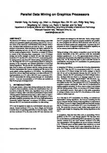
We do this as follows: For the whole recursion level j, we allocate a single stream with a total size of n2 node pairs and use certain parts of that stream as output in every phase of the algorithm as specified in Table 1. This scheme is based on the following observations: In phase 0 of a stage k, all tree nodes of the levels 0, . . . , k are modified and written. Thus any tree node of a level 0, . . . , k that has been written previous to that phase will not be further required in subsequent phases and can be overwritten safely. (Note that according to the substream specification above, tree nodes of the levels 0, . . . , k are always contained in the first 2k · 2log n−j node pairs of the stream.) Furthermore, in phase 1 of stage k, all tree nodes of level k + 1 are modified and written. Thus in this phase, all previously written nodes of level k + 1 can be overwritten. Using this scheme, the output of the last step of the merge (which was directed to the full stream of n2 node pairs) contains all 2log n−j completely modified bitonic trees of recursion level j (each of which represents a fully sorted sequence of length 2j ) in a non-interleaved manner. This stream is then used as input for the subsequent recursion level j + 1 of the adaptive bitonic sort. Since at the end of each recursion level all input tree nodes have been replaced by modified nodes in the output stream, it is sufficient to allocate two streams of n2 node pairs for the whole sort algorithm and alternately use one them as output stream in each recursion level. Fig. 1 demonstrates our output stream layout on the example of a single adaptive bitonic merge of n = 24 values. The numbers in the table specify the tree level of each node in the output stream (where 0 corresponds to the root). s is the spare node of the bitonic tree. While the node pairs shown in black are those written in the respective phase (indicated on the left), the node pairs shown in gray are the ones still accessible from previous phases. Note that the order of the nodes written in phase 0 of each stage k (shown in bold font) corresponds to an in-order-traversal of the k upper levels of the bitonic tree.
8
stage 0 0 0 0 1 1 1 2 2 3
phase 0 1 2 3 0 1 2 0 1 0
output stream layout: tree levels of node pair at stream memory location 0 1 2 3 4 5 6 7 0s 0s 11 0s 11 22 0s 11 22 33 10 1s 22 33 10 1s 22 22 33 10 1s 22 22 33 33 33 21 20 21 2s 33 33 33 21 20 21 2s 33 33 33 33 32 31 32 30 32 31 32 3s
step 0 1 2 3 4 5 6
stages 0 0 0,1 0,1 1,2 2 3
output stream layout: tree levels of node pair at stream memory location 0 1 2 3 4 5 6 7 0s 0s 11 10 1s 22 10 1s 22 22 33 21 20 21 2s 33 33 33 21 20 21 2s 33 33 33 33 32 31 32 30 32 31 32 3s
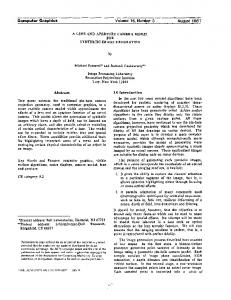
Figure 2. Output stream layout for adaptive bitonic merging of 24 values with overlapping of stages.
Figure 1. Output stream layout for adaptive bitonic merging of 24 values assuming a sequential execution of all stages.
5.4. GPU-ABiSort in O(log2 n) stream operations Since each stage k of a recursion level j of the adaptive bitonic sort consists of j − k phases, O(log n) stream operations are required for each stage. Together, all j stages of recursion level j consist of 1 2 1 2 j + 2 j phases in total. Therefore, the sequential execution of these phases requires O(log2 n) stream operations per recursion level and, in total, O(log3 n) stream operations for the whole sort algorithm. While this already allows to achieve the optimal time complexity O((n log n)/p) for up to p = n/ log2 n stream processor units, we will present in the following an improved GPU-ABiSort implementation for stream architectures that allow the specification of substreams consisting of multiple separate memory blocks, which requires only O(log2 n) stream operations for the whole sorting (and is thus theoretically capable of achieving the optimal time complexity for up to n/ log n stream processor units). The reduction of the number of stream operations by the factor O(log n) is accomplished by adapting a technique from the parallel PRAC implementation of the adaptive bitonic sorting [5]: Instead of a completely sequential execution of all stages, we execute them partially overlapped. By observing which tree levels are visited in each of the phases and in which phases they have been visited the last time before (cf. Fig. 1), we notice that phase i of a stage k can be executed immediately after phase i + 1 of stage k − 1. Therefore, we can start the execution of a new stage every other step of the algorithm (cf. [5]), which leads to an adaptive bitonic merge implementation in a total of 2 log n−1 steps and thus in O(log n) stream operations for each of the log n recursion levels of the adaptive bitonic sort.
For such an improved implementation, the previously used specification to which memory locations modified nodes are written in each phase of the algorithm (see Table 1) is still applicable. However, instead of defining a single contiguous memory block as substream in each step of the algorithm, now multiple memory blocks together form a substream that is to be used as output stream for the corresponding stream operation. In this context, the memory blocks that form a common substream correspond to those phases that can be executed in the same step of the algorithm (and thus potentially in parallel) according to the above observation. Fig. 2 shows the respective stream layout. As it can be seen there, the memory blocks belonging to a single step of the algorithm do not overlap. Finally, we can summarize the complete sorting algorithm at the stream level as follows: GPU-ABiSort: for each recursion level j of the adaptive bitonic sort, i.e. for j = 1, . . . , log n: k0 := 0 k1 := 0
(first active stage of a step of the merge) (last active stage of a step of the merge)
for each step i of the merge, i.e. for i = 0, . . . , 2j − 2: if i is even (and i > 0): increment k0 by 1 if i >= log n: decrement k1 by 1 the substream to be used as output in this step is defined by the memory blocks according to Table 1 belonging to the following phases: stage k0 phase i − 2k0 , stage k0 + 1 phase i − 2(k0 + 1), ..., stage k1 phase i − 2k1 invoke a kernel on all elements of that substream (which performs a step of the adaptive min/max determination and updates child pointers, cf. Section 5.2)
9
6. GPU-specific details 6.1. Distinctness of input and output streams In the preceding section, we assumed that it is possible to use the same stream as input and output of a stream operation. However, on current GPUs input and output streams must always be distinct (and it is currently not sufficient to use just distinct substreams from the same stream for input and output). For the stream holding the temporary node pointers p and q (see Section 5.1) we apply the pingpong technique commonly used in GPU programming: We allocate two such streams and alternately use one them as input and the other one as output stream. For the stream holding the modified node pairs (see Section 5.2) this technique cannot be applied since not all stream elements are modified in each step of the algorithm. Therefore, in our current implementation, we allocate two such streams and permanently use one of them as input and the other one as output stream. After each step of the algorithm, all nodes that have just been written to the output stream are simply copied back to the input stream.
6.2. GPU-ABiSort using a 2D stream layout For most applications, we can expect that the input sequence will be longer than the maximum allowed size of a 1D stream on current GPUs (cf. Section 3.2). Therefore, in our GPU implementation we have to pack our stream contents (i.e. the node pointers and node pair data) into 2D streams. We use the following simple mapping: if x is an index corresponding to the location of a node in the 1D stream, this node will be mapped to the location (x mod w, bx/wc) in the 2D stream (where w specifies the width of the 2D stream). We thereby assume that the width w is a power of two. To be able to use the stream program described in Section 5.4 with such a 2D stream without further modifications, it is necessary that the contiguous memory blocks, which define a substream, correspond to rectangular blocks of the 2D stream after the mapping. Our specification of those memory blocks according to Table 1 meets these demands: The length l of each block is a power of two. Furthermore, the start location x0 of each block is a multiple of l. Hence, if l ≤ w, then w is obviously a multiple of l, just like the start location x0 and the end location x0 + l of the block, and thus the block is located completely within a single line of
n 32768 65536 131072 262144 524288 1048576
CPU sort 12 – 16 ms 27 – 35 ms 62 – 77 ms 126 – 160 ms 270 – 342 ms 530 – 716 ms
GPUSort[9] 13 ms 29 ms 63 ms 139 ms 302 ms 658 ms
GPU-ABiSort 11 ms 21 ms 45 ms 95 ms 208 ms 479 ms
Table 2. Timings on a GeForce 6800 system. the 2D stream after the mapping. And if l ≥ w, then l as well as x0 are multiples of w, and thus the block spans the complete lines xw0 , . . . , xw0 + wl − 1 of the 2D stream after the mapping.
7. Results The usual application scenario of a sorting algorithm is the sorting of arbitrary data (e.g. records of a database) based on a sort key, in our case a 32bit floating point value. On the CPU this is implemented most efficiently by sorting an array consisting of value/pointer pairs, where the value is used as sort key and the pointer points to the corresponding data. (At least on our test machines, the alternative – namely to sort a simple pointer array whose entries point to records containing the sort key – was in general much slower.) We also implemented GPU-ABiSort in such a way that the input and the final output of the sorting is given as such an array of value/pointer pairs. Since we can assume (without loss of generality) that all pointers in the given array are unique, we can use these pointers at the same time as secondary sort keys for the adaptive bitonic merge (cf. Section 5.2). At first we tested our implementation on a PC system with an AMD Athlon-XP 3000+ CPU and an NVIDIA GeForce 6800 Ultra GPU with 256 MB memory (on arrays containing random values). We compared the performance of GPU-ABiSort with sorting on the CPU using the C++ STL sort function (an optimized quick sort implementation) as well as with the (non-adaptive) bitonic sorting network implementation on the GPU by Govindaraju et al., called GPUSort [9]. Table 2 shows the timings. We also tested our implementation on a PC system with an AMD Athlon-64 4200+ CPU and an NVIDIA GeForce 7800 GTX GPU with 256 MB memory. Table 3 shows the results.
8. Conclusions and future work We presented a novel approach for parallel sorting on stream architectures. As opposed to any previous
10
n 32768 65536 131072 262144 524288 1048576
CPU sort 9 – 11 ms 19 – 24 ms 46 – 52 ms 98 – 109 ms 203 – 226 ms 418 – 477 ms
GPUSort[9] 4 ms 8 ms 18 ms 38 ms 80 ms 173 ms
GPU-ABiSort 6 ms 9 ms 18 ms 37 ms 76 ms 165 ms
Table 3. Timings on a GeForce 7800 system. sorting approach on stream processors, it achieves the optimal time complexity O((n log n)/p). Furthermore, our approach performs also very well in practice, which is caused by a well-chosen stream memory layout and by several optimizations we incorporated into our approach. We implemented our approach on modern programmable graphics hardware (GPUs). The timings we obtained with this implementation are very promising, especially with regard to the performance improvements that can be expected with upcoming GPU generations. The implementation of our approach has shown that optimal parallel sorting on stream processors is indeed very efficient in practice. As it was said, in our implementation we assumed that the length of the input sequence is a power of two (as it was also done in GPU sorting network implementations). However, it should certainly be possible to incorporate the extension of the adaptive bitonic sorting approach to non-power-of-two sequence lengths by the use of pruned bitonic trees [5] into our approach. The efficient implementation of such an extension remains a task of future work. Finally, it would be interesting to explore to what extent the tree traversal and node modification techniques developed in this approach can be helpful for the adaption of other adaptive or hierarchical algorithms to the stream programming domain.
References [1] M. Ajtai, J. Koml´ os, and E. Szemer´edi. An O(n log n) sorting network. In Proceedings of the Fifteenth Annual ACM Symposium on Theory of Computing (STOC ’83), pages 1–9, 1983. [2] S. G. Akl. Parallel Sorting Algorithms. Academic Press, Inc., Orlando, FL, USA, 1990. [3] S. Amarasinghe. Multicores from the compiler’s perspective: A blessing or a curse? In Proceedings of the international symposium on Code generation and optimization (CGO ’05), pages 137–137, 2005. [4] K. E. Batcher. Sorting networks and their applications. In Proceedings of the 1968 Spring Joint Computer Conference (SJCC), volume 32, pages 307–314, 1968.
[5] G. Bilardi and A. Nicolau. Adaptive bitonic sorting: An optimal parallel algorithm for shared-memory machines. SIAM J. Comput., 18(2):216–228, Apr. 1989. [6] I. Buck, T. Foley, D. Horn, J. Sugerman, K. Fatahalian, M. Houston, and P. Hanrahan. Brook for GPUs: stream computing on graphics hardware. ACM Transactions on Graphics, 23(3):777–786, Aug. 2004. [7] R. Cole. Parallel merge sort. SIAM J. Comput., 17(4):770–785, Aug. 1988. see Correction in SIAM J. Comput. 22, 1349. [8] A. Gibbons and W. Rytter. Efficient parallel algorithms. Cambridge University Press, Cambridge, England, 1988. [9] N. K. Govindaraju, N. Raghuvanshi, M. Henson, and D. Manocha. A cache-efficient sorting algorithm for database and data mining computations using graphics processors. Technical report, University of North Carolina, Chapel Hill, 2005. [10] N. K. Govindaraju, N. Raghuvanshi, and D. Manocha. Fast and approximate stream mining of quantiles and frequencies using graphics processors. In Proceedings of the 2005 ACM SIGMOD international conference on Management of data (SIGMOD ’05), pages 611– 622, 2005. [11] A. Greß and G. Zachmann. GPU-ABiSort: Optimal parallel sorting on stream architectures (extended version). Technical report, Clausthal University of Technology, Feb. 2006. [12] U. J. Kapasi, W. J. Dally, S. Rixner, P. R. Mattson, J. D. Owens, and B. Khailany. Efficient conditional operations for data-parallel architectures. In Proceedings of the 33rd Annual IEEE/ACM International Symposium on Microarchitecture (Micro-33), pages 159–170, 2000. [13] P. Kipfer, M. Segal, and R. Westermann. Uberflow: a gpu-based particle engine. In Proceedings of the 2004 ACM SIGGRAPH/Eurographics conference on Graphics hardware (EGGH ’04), pages 115–122, 2004. [14] P. Kipfer and R. Westermann. Improved GPU sorting. In M. Pharr, editor, GPU Gems 2: Programming Techniques for High-Performance Graphics and General-Purpose Computation, pages 733–746. Addison-Wesley, 2005. [15] L. Natvig. Logarithmic time cost optimal parallel sorting is not yet fast in practice! In Proceedings Supercomputing ’90, pages 486–494, 1990. [16] J. Owens. Streaming architectures and technology trends. In M. Pharr, editor, GPU Gems 2: Programming Techniques for High-Performance Graphics and General-Purpose Computation, pages 457–470. Addison-Wesley, 2005. [17] J. D. Owens. Computer Graphics on a Stream Architecture. PhD thesis, Stanford University, Nov. 2002. [18] T. J. Purcell, C. Donner, M. Cammarano, H. W. Jensen, and P. Hanrahan. Photon mapping on programmable graphics hardware. In Proceedings of the 2003 Annual ACM SIGGRAPH/Eurographics Conference on Graphics Hardware (EGGH ’03), pages 41–50, 2003.