2008 International Joint Conference on Neural Networks Hong Kong, June 1-6, 2008
Hidden-Markov Model based Sequential Clustering for Autonomous Diagnostics Akhilesh Kumar, Finn Tseng, Yan Guo, and Ratna Babu Chinnam
Abstract— Despite considerable advances over the last few decades in sensing instrumentation and information technology infrastructure, monitoring and diagnostics technology has not yet found its place in health management of mainstream machinery and equipment. The fundamental reason for this being the mismatch between the growing diversity and complexity of machinery and equipment employed in industry and the historical reliance on “point-solution” diagnostic systems that necessitate extensive characterization of the failure modes and mechanisms (something very expensive and tedious). While these point solutions have a role to play, in particular for monitoring highly-critical assets, generic yet adaptive solutions, meaning solutions that are flexible and able to learn on-line, could facilitate large-scale deployment of diagnostic and prognostic technology. We present a novel approach for autonomous diagnostics that employs model-based sequential clustering with hiddenMarkov models as a means for measuring similarity of timeseries sensor signals. The proposed method has been tested on a CNC machining test-bed outfitted with thrust-force and torque sensors for monitoring drill-bits. Preliminary results revealed the competitive performance of the method.
C
I. INTRODUCTION
ondition Based Maintenance (CBM) is a philosophy that applies sensors to equipment for the purposes of monitoring, diagnostics, and prognostics, to facilitate optimal maintenance. CBM has the potential to greatly reduce costs by helping to avoid catastrophic failures and by more efficiently determining the intervals required for maintenance schedules [1]. The economic ramifications of CBM are many fold since they affect labor requirements, replacement part costs, routine maintenance scheduling, increased capacity, enhanced logistics, and supply chain performance [1, 2]. Despite considerable advances over the last few decades in sensing instrumentation, signal processing algorithms, and information technology infrastructure, monitoring and diagnostics technology has Manuscript received December 15, 2007. A. Kumar is a doctoral student in the Industrial & Manufacturing Engineering Department, Wayne State University, Detroit, MI 48202 USA (e-mail:
[email protected]). F. Tseng is with Research and Advanced Engineering, Ford Motor Company, Dearborn, MI 48121 USA (e-mail:
[email protected]). Y. Guo is a doctoral student in the Industrial & Manufacturing Engineering Department, Wayne State University, Detroit, MI 48202 USA (e-mail:
[email protected]). R.B. Chinnam is an Associate Professor in the Industrial & Manufacturing Engineering Department, Wayne State University, Detroit, MI 48202 USA (phone: 313-577-4846; fax: 313-578-5902; e-mail:
[email protected]).
not yet found its place in health management of mainstream machinery and equipment [6]. It is estimated by the Center for Intelligent Maintenance Systems that over $35 billion per year could be saved in the United States alone if CBM technology were to be widely employed [3]. Diagnostics is the process of identifying, localizing, determining, and classifying the severity of equipment failure, whereas prognostics is the process of predicting the remaining-useful-life (RUL) [4]. Diagnostics is not only important but is a prerequisite for effective prognostics. The primary challenge is to achieve high degree of accuracy in reasoning out the health-state of the equipment given the sensory signals. The major technical challenges with effective diagnostics are as follows [1]: 1) Sensory signal statistics tend to be quasi-stationary and vary as a function of operating conditions and ambient conditions, 2) Machine character can be quite variable due to differences in machining, part-size variations, fastener tightness, wear variations, replacement-part variations, and aging, and 3) Features indicative of machine health can be obscured by signals from other sources, multitude of transmission paths, and by noise. In addition, historical datasets and cases when available for building diagnostic algorithms tend to be limited and not “labeled” in terms of fault progression and severity. CBM diagnostic techniques must be robust and effective under these conditions. The traditional methods for diagnostics, leading to “point solutions”, can be broadly grouped into two categories: physics (or mechanistic) based and empirical based [2]. The physics based methods involve extensive characterization of equipment to understand the different failure modes and their mechanisms, something tedious and resource intensive. Sensor selection, mounting, and feature selection are equally important and demanding issues. Physics based methods are economically justified when dealing with equipment that is pervasive (e.g., motors, pumps, generators, gear boxes and so on) and/or mission critical. The empirical methods often involve tracking of few critical features (based on failure mode) combined with simplistic thresholds set from experience. The extant literature is vast and reports good success in developing these point solutions [5, 6]. However, we need cost-effective technologies for monitoring a widearray of equipment that is neither mission-critical nor pervasive. A further complicating factor is that industry, partly attributable to a growing push for mass customization, is building and employing more and more “custom” equipment, mostly ruling out the traditional “point solution” method. The goal then is to develop “generic” diagnostic and prognostic algorithms that are rapidly configurable, and
adaptive (i.e., learn on-line using unsupervised learning algorithms) to facilitate effective and efficient large-scale deployment of CBM technology for a wide variety of equipment/assets. A study by NIST concluded that the availability of “generic” methods for effective diagnostics and prognostics and their reliability is a prerequisite for widespread deployment of CBM technology [7]. The concept of autonomous diagnostics is based on unsupervised techniques. The term “unsupervised” implies ability to learn on-line without human supervision. Autonomous diagnostic methods learn gradually from the system onto which they are deployed. If developed successfully, they can be deployed onto a variety of systems with ease, without requiring much equipment specific finetuning. This paper presents a practical framework for autonomous diagnostics based on Hidden Markov Models (HMMs). HMM is a finite-state machine that is also a doubly stochastic process involving at least two levels of uncertainty: a random process associated with each state, and a Markov chain, which characterizes the probabilistic relationship among the states in terms of how likely one state is to follow another [8]. HMMs are known for their application in temporal pattern recognition such as automatic speech recognition [9, 10], handwriting, gesture recognition, musical score following, economic and financial series analysis [11], and bioinformatics (e.g., EEG time-series clustering [12] and gene expression clustering [13]). Given the success of HMMs with these applications, in particular with speech recognition that has a lot of similarity to machine diagnostics, there is great hope that they will be equally effective in diagnostic applications. Two sidebenefits are the existence of computationally efficient methods for system identification and computing of likelihoods using HMMs. They can also be used to build data-driven models of machines relieving somewhat the need to identify specific features in data to be used as health indicators [1]. We should however note that there are some notable differences between speech recognition and machine diagnostics [1]. For example, in speech processing the number of phonemes is a relatively small finite set. Furthermore, words which are constructed as sequences of phonemes also represent a finite (although large) set. These facts allow speech processors to create libraries of sounds and words which can be used to build HMMs. By comparison, the collection of machine signatures for a single machine may be very large and, of course, each machine will make different signatures. In spite of this, the literature reports good results from application of HMMs for machine monitoring and diagnostics [1-2, 14-27]. However, almost all of this literature treats the task of developing diagnostics models as one of building classification models (i.e., supervised learning) relying on labeled training histories/datasets (in terms of fault progression and severity). On the contrary, our goal is to build HMM models for diagnostics while working with unlabeled datasets, necessitating a “clustering” approach. Few notable exceptions are [2, 26, 27]. [2, 26]
suggested a hierarchical HMM approach to overcome the need for labeled datasets. However, the hierarchical HMM structure can create rigidity in building the overall diagnostics model. [26] suggested a competitive learning approach for building the diagnostic model using HMMs. However, the competitive learning process is tedious in particular with HMMs and there are issues with convergence and initialization. This paper proposes a relatively simple yet more flexible and robust approach for autonomous diagnostics in dealing with incipient failures using HMMs through a sequential clustering approach in the presence of unlabeled datasets/histories. The underlying assumption is that the sensor signals are in the form of time-series segments (univariate or multivariate). While the manuscript focuses on monitoring cutting tools on CNC machines (in particular drill bits) using a dynamometer to monitor thrust-force and torque on the cutting tool, the framework is relevant for monitoring a wide variety of equipment (e.g., rotary equipment employing vibration sensors) but might involve some signal pre-processing and or feature selection. While the monitored unit could be a component, sub-system, or a whole piece of equipment, without loss of generality, the rest of this manuscript generally refers to the monitored unit as an asset or equipment. Rest of the paper is organized as follows: section 2 briefly presents the background of HMM. Proposed framework is discussed in section 3. Experimentation and results have been presented in section 4. Finally, conclusion and future research in section 5. II. BACKGROUND OF HIDDEN-MARKOV MODELS Hidden Markov model (HMM) is a finite-state machine that is also a doubly stochastic process involving at least two levels of uncertainty: a random observation process associated with each hidden-state, and a Markov chain, which characterizes the probabilistic relationship among the states in terms of how likely one state is to follow another [8]. Note here that the “hidden state” of a HMM is not the same as the “health-state” of an equipment under diagnosis. In fact, in the proposed approach, a complete HMM will model a single health-state. In working with HMMs, the objective is to either characterize the hidden-states given the observation sequence or calculate the likelihood of the sequence given the HMM. Let X t denote the hidden state at time t and Ot the corresponding observation. Assuming that there are k possible states, we have X t ∈ {1,..., k } . Let {o1 , o2 ,...oT } denote the observation sequence of random variable Ot . Note that oi can be univariate or multivariate and that the length of the observation sequence, T, can be arbitrary. Characterization of a HMM is done through its parameters, λ = (π , A, B ) . The parameters for a basic (first-order) HMM are the initial state distribution π (i ) = P( X 1 = i ) , the transition model A = {α i , j } = P( X t = j | X t −1 = i ) , and the
observation model b j (ot ) = P (Ot = ot | X t = j ) , which is the probability of a particular observation vector at a particular time t for state j . The complete collection of parameters for all observation distributions is represented by B = {b j (⋅)} . A flexible representation of P (Ot | X t ) as a
mixture of Gaussians for observation vectors in ℜ L is [28]: P (Ot = ot | X t = i ) = M
∑ P( M m =1
t
= m | X t = i ) N (ot ; μ m ,i , Σ m ,i )
where N (ot ; μ m ,i , Σ m ,i ) is the Gaussian density with mean
μi and covariance Σi , M t the hidden variable that specifies the mixture components, and P( M t = m | X t = i ) = ci , m the conditional prior weight of each mixture component. Estimation of parameters λ = (π , A, B ) is normally carried out through an iterative learning process. A-priori values of π , A and B are assumed and observation sequences are presented iteratively to the model for parameter estimation. All the results reported in this paper are based on the use of the Baum-Welch’s Expectation Maximization algorithm [29]. Estimation of p(O | λ ) from given O = (o1 ,..., oT ) is obtained using either the Forward procedure or the Backward procedure of the FB-algorithm [30]. Estimation of p(O | λ ) is essential in building a HMM-based classifier. All our implementations are based on Kevin Murphy’s Bayesian network toolbox (for MATLAB), available at http://www.cs.ubc.ca/~murphyk/Software/BNT/bnt.html. III. PROPOSED FRAMEWORK: AUTONOMOUS DIAGNOSTICS THROUGH HMM BASED SEQUENTIAL CLUSTERING As noted earlier, our objective is to develop effective diagnostic methods for tracking incipient equipment failures given unlabeled historical datasets (i.e., sensor signal histories). Given signal histories from identical assets that have undergone a particular type of incipient failure (i.e., distinct failure mode), the goal is to characterize the distinct health-states of the asset during the degradation from a state of perfect health to a state of total failure. This is critical to facilitate timely and optimal condition-based maintenance. Given that there exist no labeled target outputs within the historical degradation datasets, we rule out the possibility of building a diagnostic classifier through supervised learning. Instead, we shall rely on unsupervised learning, in particular, clustering. We can however do better than pure clustering. While the historical datasets do not have labeled target outputs during the degradation process, they do provide us with the knowledge that the equipment was perfectly healthy at the very beginning and that the equipment has failed at the end. Given this information, we recommend a sequential clustering approach to exploit this limited information. More accurately, we are proposing a model-based sequential clustering approach to develop the
diagnostic model. For reasons outlined in the introduction section, we are relying on HMMs to perform this modelbased clustering. Let us suppose that the sensor signal historical dataset available for building the diagnostic model covers from infancy to failure the signal history of several identical pieces of equipment. Under the reasonable assumption that these assets are virtually identical during their infancy, we build the “excellent” health-state HMM model using data from the earliest stages of the asset signal history. Thus, we combine the partial histories from the infancy stage of all the assets to characterize the equipment dynamics through a single HMM (i.e., the HMM parameters are optimized to improve the “log-likelihood” for these infancy stage signals). While characterization of the excellent health-state is some what straightforward, this is not the case for the remaining health-states. Given the complexity of these assets, it is typical for equipment even from an identical asset class to exhibit significant variation in the degradation process even under an identical failure mode. As noted earlier, this is attributable to such factors as differences in machining, part-size variations, fastener tightness, wear variations, replacement-part variations, and aging. Thus, we cannot simply take sample histories based on asset age or usage to train HMMs for subsequent health-states. We instead take the following approach to characterize these states. As expected, the similarity between the trained “excellent” health-state HMM and the asset signal history, measured in terms of log-likelihood, will decrease as the asset progresses from a state of perfect health to a state of total failure. Candidate partial signal histories for characterizing the “next best” health-state can be identified by studying the log-likelihood profiles from the “excellent” health-state HMM. We first expose the complete signal history of each asset, one asset at a time, to the trained excellent health-state HMM. Statistical characterization of the log-likelihood distribution based on signals from the infancy stage alone (i.e., training data for the excellent health-state HMM) will allow determination of a minimum log-likelihood threshold or cutoff, beneath which, we can declare that there is “poor” similarity between the excellent health-state HMM model and the signal. We then identify candidate sample histories for training the “next best” health-state by identifying signal histories that come close but fail to meet the log-likelihood threshold. These sample histories are then pooled to train another HMM for characterization of the “next best” health-state. The process can be repeated until all the signal histories from the asset family have been used to model the distinct health-states. It should be noted that the resolution of the characterization of the different health-states for a given failure mode will be a function of the criteria for establishing the log-likelihood thresholds (the higher the thresholds the higher the resolution). While high resolution is desired, given the inevitable noise present within the signal histories, accuracy will be compromised at very high resolutions. The rest of this section details this overall process.
A. Sequential Clustering of Historical Data Let us suppose that sensor signal histories are available for N identical assets subject to a common failure mode (O1 , O2 ,..., ON ) . The sensor signal history from asset n is of the form On = {on,1 , on,2 ,...on ,Tn } , where on ,1 , on,2 ,...on ,Tn constitutes time-series segments sampled from the asset at regular intervals of time or usage (number of segments available from different assets until failure could be different depending the rate of degradation). Thus, on ,1 is the first time-series historical segment from asset n . Note again that these time-series segments can be univariate or multivariate depending on the number of sensors mounted on the asset and the signal processing and feature extraction procedures employed. The following steps are involved in sequential clustering of these signal histories using HMMs for building the diagnostic model: Step1- Initialization: The proposed algorithm initiates with construction of an HMM λ1 with a pre-specified configuration, with the configuration to be “optimized” using cross-validation procedures outlined later. The parameters of HMM λ1 (i.e., π , A and B ) are initialized using infancy signal history from a random asset i (e.g., oi ,1 or oi ,2 ). Step2- Characterize “Excellent” Health-state: We train HMM λ1 to adjust ( π , A , B ) towards maximizing p(O | λ ) . For training, signals from earliest stages of the asset’s life are considered, e.g. oi ,1 or oi ,2 of all N assets. Because of
such factors as “wear-in”, our research suggests that oi ,2 or oi ,3 can be more reliable than oi ,1 for characterizing the “excellent” health-state (depending of course on such as factors as time-between two consecutive samples and typical life of the asset). Once trained, all N sequences are evaluated with this trained HMM and similarity is observed based on log-likelihood values, in particular, their distribution. The log-likelihood similarity threshold or cutoff for characterizing the “next” health-state is set at μ − kσ , where μ and σ denote the mean and standard deviation of the log-likelihood value distribution, respectively, and k an integer. The higher the value of k the lower the resolution of characterization of the different health-states. Step 3- Identify Candidate Signals for Characterizing “Next” Health-State: Segments from each asset i that just missed the log-likelihood threshold of the previous healthstate are identified as candidate training signals for the “Next” health-state. A new HMM λ2 is constructed and trained with these newly identified training signal segments. Step 4- Termination: Step 3 is repeated until all sensor signal segments of each asset have been characterized. B. Labeling Health-states based on HMM Clusters Let us suppose that the sequential clustering process yielded M distinct health-state HMMs, representing the distinct temporal dynamics of the sequences that make up the
respective clusters. Thus, each HMM represents one healthstate sequentially from “Excellent” to “Failure”. C. On-line Diagnostics using HMM-Based Classifier Now that the distinct health-sates are characterized, in an on-line diagnostics setting, given the sensor signal segment, determination of the “current” health-state involves calculation of the log-likelihood with respect to all characterized HMMs. The health-state corresponding to the HMM with the largest log-likelihood is the estimated healthstate. IV. CASE STUDY: DIAGNOSTICS IN A DRILLING PROCESS A. Experimental Setup Drilling process, one of the most commonly used machining processes, is selected here as a test-bed for validating the proposed autonomous diagnostics framework. The diagnostics objective is to assess the health or well-being of the drill-bit during the machining process by utilizing thrustforce and torque signals captured by a dynamometer during the drilling cycle (constituting a logical sensor signal segment). Tests were conducted on HAAS VF-1 CNC Machining Center with Kistler 9257B piezo-dynamometer (sampled at 250Hz) to drill holes in ¼ inch stainless steel bars. High-speed twist drill-bits with two flutes were operated at feed rate of 4.5 inch/minute and spindle-speed at 800 rpm without coolant. Each drill-bit was used until it reached a state of physical failure either due to excessive wear or due to gross plastic deformation of the tool tip due to excessive temperature (resulting from excessive wear). Twelve drill-bits were used to generate the signal histories necessary for building the diagnostics model. The shortest drill-bit lasted 16 holes and the longest 23 holes. B. Observation Sequence A sequence is defined here as one that covers an individual hole. Due to bit wear and non-uniformity of the work piece surface, the actual time necessary to drill a hole varies. This results in sequences of different lengths. Thrust-force (Newtons) and torque (Newton-meters) signal amplitudes are usually quite different. To improve the convergence properties of the EM algorithm used for training the HMMs, the observational sequences are all normalized to mean zero and standard deviation of unity for both thrust-force and torque. Observation sequences that are presented to HMMs are not subjected to any transformation other than this normalization. Figure 1 illustrates a joint plot of normalized thrust-force and torque signals during a particular hole.
average without ever risking failure within a work-piece. On the contrary, a simple “static” policy of replacing the drillbit after the average life of 19 holes would have resulted in 4 failures and lost the ability to produce 11 holes. A more conservative policy of replacing the drill-bits after 15 holes, based on the earliest witnessed failure (drill-bit #4), would have lost the ability to produce 50 holes, yielding a utilization of just 78% of useful-life.
1.5
Normalized Torque
1 0.5 0 -0.5 -1 -1.5
End
TABLE I HEALTH-STATE REPRESENTATION Hole #
Start
-2 -2
-1
0 1 Normalized Thrust
2
1 2 3 4 5 6 7 8 9 10 11 12 13 14 15 16 17 18 19 20 21 22 23
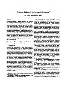
C. Labeling Health-states As discussed in section III.A, proposed algorithm initially characterizes “excellent” health-state using signal segments from the second hole of the drill-bit set. Figure 2 shows the log-likelihood plot for the trained excellent health-state HMM configured with two hidden-states. 500 Excellent Health-State HMM
Log-Likelihood
0 -500 -1000 -1500 -2000 0
5
10
15
20
25
30
Hole #
Fig. 2. Log-likelihood plot of “Excellent” health-state with two hidden-states.
Continuing with the steps outlined in Section III.A, the rest of the health-states are characterized as well, using k = 2 for establishing the log-likelihood threshold. Table 1 gives the results of health-state estimation for all drill-bits using the proposed algorithm. Overall, the process has yielded three health-states (“F” indicates the failed hole, part of health-state “3”). While different drill-bits have spent different number of holes in the different health-states, all drill-bits have gone through all the three health-states prior to failure. What is particularly interesting and quite valuable is the knowledge that drill-bits spent on the average 55% of the time in healthstate 1, 25% in health-state 2, and only 21% in health-state 3. Thus, enhancing the value of tracking the health-state of the drill-bit on-line for efficient replacement. For example, a “dynamic” policy of replacing the drill-bit once entering the final health-state would not have resulted in any failures while only losing the ability to produce 26 holes successfully, assuming that these 12 drill-bits are representative of the overall population. This translates to utilization of 89% of the useful-life of the drill-bits on the
Drill Bits
Fig. 1. Joint plot of normalized thrust-force and torque signals during a particular hole. Note the overall shape in spite of local randomness.
1 2 3 4 5 6 7 8 9 10 11 12
1 1 1 1 1 1 1 1 1 1 1 1
1 1 1 1 1 1 1 1 1 1 1 1
1 1 1 1 1 1 1 1 1 1 1 1
1 1 1 1 1 1 1 1 1 1 1 1
1 1 1 1 1 1 1 1 1 1 1 1
1 1 1 1 1 1 1 1 1 1 1 1
1 1 1 1 1 1 1 1 1 1 1 1
1 1 1 1 1 1 1 1 1 1 1 1
1 1 1 2 1 1 1 2 1 1 1 1
1 1 1 2 1 2 1 2 1 1 1 1
1 1 1 2 2 2 1 2 1 1 1 1
1 2 2 2 2 2 2 3 1 1 1 2
1 2 2 2 2 2 2 3 1 1 1 2
2 2 2 3 2 3 2 3 2 1 2 2
2 2 2 3 2 3 2 3 2 1 2 2
2 2 2 F 2 3 2 3 2 2 2 3
2 2 2 3 F 2 3 3 F 3 3 3 F 3 F 2 3 2 2 2 3
3 F 2 3 3 2 2 3
3 F 3 2 3 3
F 3 3 3 3
3 3 F 3 3 F 3 3 F F
D. Cross-Validation and Testing Process While the results reported in Section IV.C are very good, they are not necessarily reproducible. This is attributable to the fact that data from all the drill-bits were employed for building the diagnostic model as well as testing its performance. To evaluate the generalization performance of the proposed method, we now report results from crossvalidation and testing experiments. In addition, one has to optimize the configuration of the HMM structure as well, in particular, the specification of the number of hidden-nodes, Q . In all our experiments, we assumed that the observation model is a Gaussian distribution and no conditions were imposed on the state-transition matrix. The 12 drill-bits are now separated into 2 groups, training group consisting of 9 drill-bits and 3 drill-bits in the testing group. The training group will be further subject to a 9-fold cross-validation procedure, where 8 drill-bits will be used for performing the sequential clustering and characterizing the health-states while the model will be tested on the leftout drill-bit. This procedure is repeated nine times, leaving out a different drill-bit every time for cross-validation. In addition, we repeat the whole process leaving out different combinations of the 3 drill-bits for testing 12 ( C3 = 220 combinations). Convergence: The convergence evaluation criteria are as follows: 1) No "reverse jumps", meaning that the drill-bit cannot enter a state and then revert to a previous state. If 2 or more reverse jumps are noticed in the validation cycle, the model building run will be terminated. 2) At least two health-states have to be detected. If during the sequential clustering process no more than 1 HMM model was obtained, the run would be terminated.
for each value of Q is C312 = 220 × 9 (for full s-fold crossvalidation) = 1980. Figures 3, 4, and 5 clearly suggest that for this application, two hidden-states are best for configuring the HMMs for health-state characterization. Not only is the overall performance best with two hidden-states, the detection rate S (Q) is also highest for Q = 2. The overall performance is quite impressive at nearly 98%, even under testing. In theory, it is also possible to vary Q for the different health-state HMM models. 0.99
Success Rate
0.98 0.97 0.96
0.995
Detection Rate
0.99
0.98 0.975 0.97 1
2
3
4
5
6
7
8
6
7
8
Number of Hidden States
Fig. 4. Plot of Q vs. S (Q) . 0.98 0.97 0.96 0.95 0.94 0.93 0.92 0.91 0.9 1
2
3
4
5
Number of Hidden States
Fig. 5. Plot of Q vs. P (Q) .
V. CONCLUSIONS AND FUTURE RESEARCH In the context of condition-based maintenance, the proposed framework allows us to overcome the tedious and often impossible task of “labeling” dataset health-states, and hence, improves autonomy of techniques for diagnostics. On the contrary, traditional HMM based diagnostics framework employs a “classification” framework that strictly requires labeling. The results from the drilling process case study are extremely satisfactory. The framework was able to successfully cluster and recognize variable length and bivariate time-series sequences that are non-stationary in nature. It is not clear at this point if this framework will yield satisfactory results when spectral properties are of more importance over temporal aspects of the sensory signals. However, the speech processing community has successfully employed HMMs for modeling dynamics of spectral features derived from speech signals. Future research will study other types of rotary equipment as well as different sensor settings. Extensions for supporting prognostics will also be a priority.
0.95
REFERENCES
0.94
[1]
0.93 0.92 1
0.985
Overall Performance
For each Q , the fraction of successfully finished runs (trainings) is saved as F (Q) . Performance Criteria: The performance is judged based on the 3 drill-bits in the testing group. Three criteria are taken into account: 1) Fraction number of runs that did not produce any reverse jumps, R (Q) . 2) Fraction number of drill-bits that did enter all the identified health-states characterizing the degradation from a state of perfect health to a state of total failure, M (Q) . 3) Fraction number of impending failures detected in advance, S (Q) . Meaning, at least two of the last three holes of any testing drill-bit should be recognized to be part of the last health-state. Given the number of hidden-states, Q , combining these three performance metrics (i.e, R (Q) , M (Q) , and S (Q) ) with F (Q) yields an overall performance measure. While it is certainly possible to increase the importance of certain measures over others (e.g., it is probably more appropriate to increase emphasis on S (Q) ), we chose the following multiplicative model: P (Q) = R(Q) ⋅ M (Q) ⋅ S (Q) ⋅ F (Q) In our tests, we reasonably varied the number of hiddenstates, Q , from 2 to 8. The total number of attempted runs
2
3
4
5
6
Number of Hidden States, Q
7
8
[2]
Fig. 3. Plot of Q vs. F (Q) .
[3] [4]
C. Bunks, D. McCarthy, and T. Al-Ani, “Condition-based maintenance of machines using hidden Markov models”, Mechanical Systems & Signal Processing, vol. 14, 2000, pp. 597-612. F. Camci, “Autonomous, Process Monitoring, Diagnostics, and Prognostics Using Support Vector Machines and Hidden Markov Models”, Ph.D. Dissertation, Industrial and Manufacturing Engineering, Wayne State University, Detroit, MI, USA, 2005. Harbor Research Pervasive Internet Report, “Approaching Zero Downtime”, The Center for Intelligent Maintenance Systems, April 2003. K. Maynard, C. S. Byington, G. W. Nickerson, and M. V. Dyke, “Validation of Helicopter Nominal and Faulted Conditions Using Fleet Data sets”, Proc. of the Intnl. Conf.on Condition Monitoring, UK, 1999, pp. 129 –141.
[5]
C. Begg, T. Merdes, C.S. Byington, and K.P. Maynard, “Mechanical System Modeling for Failure Diagnostics and Prognosis”, Proc. of Maintainability and Reliability Conference (MARCON 99), Gatlinburg, Tennessee, May 10-12, 1999. [6] G. J. Kacprzynski and M. J. Roemer, “Health Management Strategies for 21st Century Condition-Based Maintenance Systems,” 13th International Congress on COMADEM: Condition Monitoring and Diagnostic Engineering Management, Houston, TX, December 3-8, 2000. (http://www.ascturbo.com/download/HMStrategies.PDF) [7] NIST-ATP, “NIST-ATP Workshop on Condition-Based Maintenance”, NIST-ATP CBM Workshop Report, Atlanta, GA November 1998. [8] “Hidden Markov Model”. McGraw-Hill Dictionary of Scientific and Technical Terms. Retrieved December 10, 2007, from Answers.com Web site: http://www.answers.com/topic/hidden-markov-model [9] I. Sanches, “Noise-compensated hidden Markov models”, IEEE Transactions on Speech and Audio Processing, vol. 8, 2000, pp. 53340. [10] B. D. Womack and J. H. L. Hansen, “N-channel hidden Markov models for combined stressed speech classification and recognition”, IEEE Transactions on Speech and Audio Processing, vol. 7, 1999, pp. 668-77. [11] S. M. Focardi, “Clustering economic and financial time-series: Exploring the existence of stable correlation conditions”, The Intertek Group, 2005. [12] A.B. Geva, and D.H. Kerem, “Brain state identification and forecasting of acute pathology using unsupervised fuzzy clustering of EEG temporal patterns”, in Fuzzy and Neuro-Fuzzy Systems in Medicine, edited by H Teodorescu, A Kandel and L C. Jain, CRC Press: USA, 1998, pp. 57–93. [13] Z. Joseph, G. Gerber, D. Gifford, and T. Jaakkola, “A new approach to analyzing gene expression time-series data”, in The Sixth Annual International Conference on Research in Computational Molecular Biology, 2002. [14] L. P. Heck and J. H. McClellan, “Mechanical system monitoring using hidden Markov models”, Proc. Int. Conf. Acoustics, Speech, Signal Processing, 1991, pp. 1697- 1700. [15] P. Smyth, “Hidden Markov models for fault detection in dynamic systems”, Pattern Recognition vol. 27, no. 1, 1994, pp. 149–164. [16] P. Smyth, “Markov monitoring with unknown states”, IEEE Journal on Selected Areas in Communications, vol. 12, no. 9, 1994, pp. 1600– 1612. [17] L.M.D. Owsley, L.E. Atlas, and G.D. Bernard, “Self-organizing feature maps and Hidden Markov models for machine tool monitoring”, IEEE Transactions on Signal Processing, vol. 45, no. 11, 1997, pp. 2787– 2798. [18] Y. Zhang, X.R. Li, and K. Zhou, “A fault detection and diagnosis approach based on Hidden Markov chain model”, Proceedings of the American Control Conference, Philadelphia, (June 1998), pp. 2012– 2016. [19] G.E. Hovland and B.J. McCarragher, “Hidden Markov models as a processor monitor in robotic assembly”, The International Journal of Robotics Research, vol. 17, no. 2, 1998, pp. 153–168. [20] H. M. Ertunc , K. A. Loparo, and H. Ocak, “Tool wear condition monitoring in drilling operations using hidden Markov models (HMMs),” Int. J. Mach. Tools Manufact., vol. 41, 2001, pp. 13631384. [21] L. Atlas , M. Ostendorf, and G. D. Bernard “Hidden Markov models for monitoring machine tool wear,” Proc. Int. Conf. Acoustics, Speech and Signal Processing, 2001, p. 3887-3890. [22] L. Wang , M. G. Mehrabi, and E. Kannatey Asibu, Jr. “Hidden Markov model-based tool wear monitoring in turning,” J. Manufact. Sci. Eng., vol. 124, 2002, pp. 651-658. [23] P. Baruah and R. B. Chinnam, “HMMs for diagnostics and prognostics in machining processes”, International Journal of Production Research, vol. 43, 2005, pp. 1275-1293. [24] R. B. Chinnam and Fatih Camci, “Hierarchical HMMs for autonomous diagnostics and prognostics”, presented at IEEE International Joint Conference on Neural Networks 2006. [25] O. Cetin, M. Ostendorf, G.D. Bernard, “Multirate Coupled Hidden Markov Models and Their Application to Machining Tool-Wear
Classification”, IEEE Transactions on Signal Processing, vol. 55, no. 6, 2007, pp. 2885-2896. [26] F. Camci and R.B. Chinnam, “Health-State Estimation and Diagnostics in Machining Systems using Hidden Markov Model Committees,” Proc. of 15th International Conference on Flexible Automation Intelligent Manufacturing, Bilbao, Spain, July 18-20, 2005. [27] R.B. Chinnam and P. Baruah, “Autonomous Diagnostics and Prognostics through Competitive Learning Driven HMM-Based Clustering,” Proc. of IJCNN'03 International Joint Conference on Neural Networks, Portland, OR, July 20-24, 2003. [28] K. Murphy, “Dynamic Bayesian Network: Representation, Inference, and Learning”, PhD. Dissertation, University of California, Berkeley, 2002. [29] A.B. Poritz, “Hidden Markov Models: A Guided Tour”, in ICASSP, 1988. [30] J. Blimes, “A Gentle Tutorial of the EM Algorithm and its Application to Parameter Estimation for Gaussian Mixture and Hidden Markov Models”, Technical Report, University of Berkeley, USA, 1988.