SZd(i) : x. Sl,(i) : x. S:,(w) : x . where p"(i) is the ancestor of wi of a generations (scales),. ~"(i) is the set of descendants of wi of (Y generations. (scales), and s;(i) ...
HIERARCHICAL MARKOV MODELS FOR WAVELET-DOMAIN STATISTICS Z. Azimifar
II Fieguth
E. Jemigan
Department of Systems Design Engineering University of Waterloo Waterloo, Ontario, Canada, N2L-3G1 ABSTRACT There is a growing realization that modeling wavelet coefficients as statistically independent may be a poor assumption. Thus, this paper investigates two efficient models for wavelet coefficient coupling. Spatial statistics which are Markov (commonly used for textures and other random imagery) do not preserve their Markov properties in the wavelet domain; that is, the wavelet-domain covariance P, does not have a sparse inverse. The main theme of this work is to investigate the approximation of P, by hierarchical Markov and non-Markov models.
1. INTRODUCTION Wavelet shrinkage is a widely-used and effective method for image modeling and enhancement problems. However, virtually all wavelet marginal models currently being used in wavelet shrinkage [7] assume the coefficients to be decorrelated and treated individually. Although such independent models result in simple nonlinear shrinkage algorithms, this approach is not optimal in the sense that for most spatial statistics or prior models the wavelet transform is not a perfect whitener. There have been several recent approaches that examine the joint statistics of the coefficients. Xu et al. [9] used the scale dependent consistency between wavelet COefficients for the denoising process. In separate work by Simoncelli [8]and Crouse et al. (31, probabilistic models were studied that capture wavelet coefficient dependencies, mainly across scales. Crouse et al. [3] considered bidden states describing each coefficient’s significance. Instead of the coefficients values, they propose statistical models for a coefficient’s hidden state dependencies. Normally an assumption is present that the correlation between coefficients does not exceed the parent-child dependencies, e.g. given the state of its parent, a child is decoupled from the entire wavelet tree. Having been motivated by these inter-coefficient probabilistic studies, the primary goal of this work is to propose a well-structured wavelet-domain correlation model which
0-7803-7997-7/03/$17.000 2003 IEEE
258
Fig. 1. Correlation coefficients of a spatial thin-plate model in
the wavelet domain. The main diagonal blocks correspond to the same scale and orientation. whereas off-diagonal blocks illustrate aOSsCOrrelations across orientations or across scales.
is capable of describing coefficient dependency by introducing a local neighborhood containing statistics of within- and across-scale coefficients. The main novelty is the systematic approach we have taken to define a wavelet-based neighborhood system consisting of 1) inter-scale dependency evolution, 2 ) within-scale clustering, and 3) across-orientation (geometrical constraints) activities. This probabilistic modeling is directly applied to the coefficient values, hut to some extent their significance is also considered. It is well-known that the wavelet-domain covariance, P, (Figure l), is block-structured. We have observed [I] that, although the majority of correlations are very close to zero (i.e., decorrelated), a relatively significant percentage (10%) of the coefficients are strongly correlated across several scales or within a p d c u l a r scale but across three orientation subbands. One approach to statistically model these relationships was to implement a multiscale model [I]. Although the MS model captured the existing strong parentchild correlation, spatial and inter-orientation interactions are not explicitly taken into consideration. Our most recent work [2] investigated the significance of inter-orientation
and spatial relationships, which we seek to model more formally in this paper.
2. WAVELET COVARIANCE APPROXIMATION Suppose we have a smooth Gaussian Makov Random Field (MRF) prior P,, projected into the wavelet domain with wavelet prior P, as is shown in Figure 1. Following our past work in wavelet statistics [l, 21 we propose to model the wavelet coefficients not as independent, but as governed by some local stochastic process. Since correlations are present within and across scales, clearly a random field model for wavelet coefficients will need to be explicitly hierarchical. Based on the correlation map of Figure 1, six different symmetric neighborhood structures are chosen. For a coefficient wi belonging to the wavelet coefficients set IV = {E'*, W,, W,} we define
where operators d, U , and h return diagonal, vertical, and horizontal subband counterparts. With these hypothesized structures in place, the remainder of this article develops and tests two associated models. 2.1. Local Estimation
We begin with an explicitly local estimator, where only those measurements within the neighborhood are used. Thus, given the noisy measurements
yi=wi+vi,
. . ..
Sud(i): x
SZd(i)
.
: x
sl(i):
Sl,(i) :
,...,C f i ( i ) }
... . x
x
sz(i):
S:,(w)
:
... .. ...
Yi = [Yi
IV4(i) = {PZ(i),CZ(i),SZ(i)~
Y(W))l,
wi = [UJi
w(N(i))l
from which the standard estimator follows trivially
. A;,'
iKi =
. yi
(2)
and where we are only interested in
x
x
where p " ( i ) is the ancestor of wi of a generations (scales), ~ " ( iis) the set of descendants of wi of (Y generations (scales), and s ; ( i ) defines various sibling sets (same scale as wi). This allows us to propose six neighborhood structures:
K ( i ) = { P l ( i ) ,C l ( i ) , S l ( i ) } W i )= {PI(i),Clt9>S?(~)} &(i) = { P Z ( ~ ) > C Z ( ~ ) > ~ I ( ~ ) }
(1)
we form a local estimation problem
P d i ) = {Pl(i),..,,Pk(i)} Ck(i)={Cl(i)
W~-N(O,T~)
= E[Wi/Yi]
23. MRF-Based Estimation The second approach is to use a local model, for which P;' is sparse; that is, a Markov random field. As can easily be verified, however, in most cases the wavelet prior is not indeed, Markov, therefore an approximate Markov model needs to be estimated. Our local model ;E
Note that, in distinct contrast to the vast majority of planar MRF models in which g is stationary, the structure of the wavelet tree (asymmetry between parent and child, or between siblings) makes g rather nonstationary and considerably complicates model estimation [4, 51.
3. MODEL EVALUATION We examine six different wavelet neighborhood structures. Clearly each choice of neighborhood will differ in its statistical accuracy. The six local and MW-based results are compared with the null estimator
61. - Yi and the pointwise estimator
259
a
prior model is not stationary: It is known that a stationary prior projected into the wavelet domain, changes to nonstationay, because of the multiscale nature of the wavelet domain. In this case the complexity of the model estimation process L is O ( n . m3), because L; # L j . if j # i. Thus, the total complexity of the local estimator w = L y is
O ( n . (m3+ d)).
The computational cost for the MRF-based estimators is more complicated. In this paper, we only consider the simple linear case, i.e, Gaussian prior. Let us consider these two pieces of information, respectively the MRF prior (3) and the measurement: Gw=q y=w+v,
Fig. 2.
RMMSE noise reduction as a function of HMRF neighborhood systems used in the two approximation techniques. MRF stands far MRFbared method and Local depicts explicil local method.
with the RMMSE of all cases plotted in Figure 2. It is clear that the vast bulk of the benefit is to be obtained from relatively few coefficients in the locality of the center coefficient. Empirica~~y, the presence of within-scale (and acrossorientation) correlation in these simulations (from NI (w) towards Ns(w)) reduces the estimation error. The second aspect of comparison is computational complexity. The complexity is complicated by the presence of MRF models, which may be solved in a wide variety of ways. In increasing order of complexity we have a) Pointwise, b) Local 1-6, c) Multiscale, d) MRF 1-6, e) Full model. Clearly the pointwise method is a linear approach, known as Wiener filtering, with its complexity growing linearly as the number of wavelet coefficients n increases. On the other side, the complexity of the Multiscale-based estimator is O(d3n),where d shows dimensionality of every node (in the simplest case d = 1)[I] Let us re-write ( 2 ) to investigate the complexity of local models
. Ai,'
. yj = Liyi
1
i
n
-
N(0,Q )
Define a linear estimator to find w which minimizes
=$.
iV; =
17
v-N(O,R)
(4)
with matrix Liof size m x m, where m,