Image Segmentation by Branch-and-Mincut - Semantic Scholar

Image Segmentation by Branch-and-Mincut Victor Lempitsky, Andrew Blake, and Carsten Rother Microsoft Research Cambridge

Abstract. Efficient global optimization techniques such as graph cut exist for energies corresponding to binary image segmentation from lowlevel cues. However, introducing a high-level prior such as a shape prior or a color-distribution prior into the segmentation process typically results in an energy that is much harder to optimize. The main contribution of the paper is a new global optimization framework for a wide class of such energies. The framework is built upon two powerful techniques: graph cut and branch-and-bound. These techniques are unified through the derivation of lower bounds on the energies. Being computable via graph cut, these bounds are used to prune branches within a branchand-bound search. We demonstrate that the new framework can compute globally optimal segmentations for a variety of segmentation scenarios in a reasonable time on a modern CPU. These scenarios include unsupervised segmentation of an object undergoing 3D pose change, category-specific shape segmentation, and the segmentation under intensity/color priors defined by Chan-Vese and GrabCut functionals.

2

1

Extended technical report of ECCV-2008 publication

Introduction

Binary image segmentation is often posed as a graph partition problem. This is because efficient graph algorithms such as mincut permit fast global optimization of the functionals measuring the quality of the segmentation. As a result, difficult image segmentation problems can be solved efficiently, robustly, and independently of initialization. Yet, while graphs can represent energies based on localized low-level cues, they are much less suitable for representing non-local cues and priors describing the foreground or the background segment as a whole. Consider, for example, the situation when the shape of the foreground segment is known a priori to be similar to a particular template (segmentation with shape priors). Graph methods can incorporate such a prior for a single pre-defined and pre-located shape template[14, 21]. However, once the pose of the template is allowed to change, the relative position of each graph edge with respect to the template becomes unknown, and the non-local property of shape similarity becomes hard to express with local edge weights. Another example would be the segmentation with non-local color priors, when the color of the foreground and/or background is known a priori to be described by some parametric distribution (e.g. a mixture of the Gaussians as in the case of GrabCut [26]). If the parameters of these distributions are allowed to change, such a nonlocal prior depending on the segment as a whole becomes very hard to express with the local edge weights. An easy way to circumvent the aforementioned difficulties is to alternate the graph partitioning with the reestimation of non-local parameters (such as the template pose or the color distribution). A number of approaches [6, 17, 26, 16] follow this path. Despite the use of the global graph cut optimization inside the loop, local search over the prior parameters turns these approaches into local optimization techniques akin to variational segmentation [7, 9, 24, 29]. As a result, these approaches may get stuck in local optima, which in many cases correspond to poor solutions. The goal of this paper is to introduce a new framework for computing globally optimal segmentations under non-local priors. Such priors are expressed by replacing fixed-value edge weights with edge weights depending on non-local parameters. The global minimum of the resulting energy that depends on both the graph partition and the non-local parameters is then found using the branchand-bound tree search. Within the branch-and-bound, lower bounds over tree branches are efficiently evaluated by computing minimal cuts on a graph (hence the name Branch-and-Mincut). The main advantage of the proposed framework is that the globally optimal segmentation can be obtained for a broad family of functionals depending on non-local parameters. Although the worst case complexity of our method is large (essentially, the same as the exhaustive search over the space of non-local parameters), we demonstrate that our framework can obtain globally optimal image segmentation in a matter of seconds on a modern CPU. Test scenarios include globally optimal segmentation with shape priors where the template shape is allowed to deform and to appear in various poses as well as image segmenta-

Extended technical report of ECCV-2008 publication

3

tion by the optimization of the Chan-Vese [7] and the GrabCut [26] functionals. In all cases, bringing in high-level non-local knowledge allows to solve difficult segmentation problems, where local cues (considered by most current global optimization approaches) were highly ambiguous.

2

Related Work

Our framework employs the fact that a submodular quadratic function of boolean variables can be efficiently minimized via minimum cut computation in the associated graph [2, 11, 19]. This idea has been successfully applied to binary image segmentation [3] and quickly gained popularity. As discussed above, the approach [3] still has significant limitations, as the high-level knowledge such as shape or color priors are hard to express with fixed local edge weights. These limitations are overcome in our framework, which allows the edge weights to vary. In the restricted case, when unary energy potentials are allowed to vary and depend on a single scalar non-local parameter monotonically, efficient algorithms known as parametric maxflow have been suggested (see e.g. [20]). Our framework is however much more general then these methods (at a price of having higher worst-case complexity), as we allow both unary and pairwise energy terms to depend non-monotonically on a single or multiple non-local parameters. Such generality gives our framework flexibility in incorporating various high-level priors while retaining the globality of the optimization. Image segmentation with non-local shape and color priors has attracted a lot of interest in the last years. As discussed above, most approaches use either local continuous optimization [29, 7, 24, 9] or iterated minimization alternating graph cut and search over non-local parameter space [26, 6, 17]. Unfortunately, both groups of methods are prone to getting stuck in poor local minima. Globaloptimization algorithms have also been suggested [12, 27, 28] . In particular, simultaneous work [10] presented a framework that also utilizes branch-and-bound ideas (paired with continuous optimization in their case). While all these global optimization methods are based on elegant ideas, the variety of shapes, invariances, and cues that each of them can handle is limited compared to our method. Finally, our framework may be related to branch-and-bound search methods in computer vision (e.g. [1, 22]). In particular, it should be noted that the way our framework handles shape priors is related to previous approaches [15, 13] that used tree search over shape hierarchies. However, neither of those approaches accomplish pixel-wise image segmentation.

3

Optimization Framework

In this section, we discuss our global energy optimization framework for obtaining image segmentations under non-local priors1 . In the next sections, we detail how it can be used for the segmentation with non-local shape priors (Section 4) and non-local intensity/color priors (Section 5). 1

The C++ code for this framework is available at the webpage of the first author.

4

Extended technical report of ECCV-2008 publication

3.1

Energy Formulation

Firstly, we introduce notation and give the general form of the energy that can be optimized in our framework. Below, we consider the pixel-wise segmentation of the image. We denote the pixel set as V and use letters p and q to denote individual pixels. We also denote the set of edges connecting adjacent pixels as E and refer to individual edges as to the pairs of pixels (e.g. p, q). In our experiments, the set of edges consisted of all 8-connected pixel pairs in the raster. The segmentation of the image is given by its 0−1 labeling x ∈ 2V , where individual pixel labels xp take the values 1 for the pixels classified as the foreground and 0 for the pixels classified as the background. Finally, we denote the non-local parameter as ω and allow it to vary over a discrete, possibly very large, set Ω. The general form of the energy function that can be handled within our framework is then given by:

E(x, ω) = C(ω)+

X p∈V

F p (ω)·xp +

X p∈V

B p (ω)·(1−xp )+

X

P pq (ω)·|xp −xq | . (1)

p,q∈E

Here, C(ω) is a constant potential, which does not depend directly on the segmentation x; F p (ω) and B p (ω) are the unary potentials defining the cost for assigning the pixel p to the foreground and to the background respectively; P pq (ω) is the pairwise potential defining the cost of assigning adjacent pixels p and q to different segments. In our experiments, the pairwise potentials were taken non-negative to ensure the tractability of E(x, ω) as the function of x for graph cut optimization [19]. All potentials in our framework depend on the non-local parameter ω ∈ Ω. In general, we assume that Ω is a discrete set, which may be large (e.g. millions of elements) and should have some structure (although, it need not be linearly or partially ordered). For the segmentation with shape priors, Ω will correspond to the product space of various poses and deformations of the template, while for the segmentation with color priors Ω will correspond to the set of parametric color distributions.

3.2

Lower Bound

Our approach optimizes the energy (1) exactly, finding its global minimum using branch-and-bound tree search [8], which utilizes the lower bound on (1) derived as follows:

Extended technical report of ECCV-2008 publication

5

 min

x∈2V ,ω∈Ω

X

E(x, ω) = min min C(ω) + x∈2V ω∈Ω

F p (ω)·xp +

p∈V

 x∈2V

p,q∈E

B p (ω)·(1 − xp )+

p∈V



P pq (ω)·|xp − xq | ≥ min min C(ω) +

X

X

ω∈Ω

X p∈V

min F p (ω)·xp +

ω∈Ω

 X p∈V

min B p (ω)·(1 − xp ) +

ω∈Ω

X p,q∈E

min P pq (ω)·|xp − xq | =

ω∈Ω

 min CΩ +

x∈2V

 X p∈V

FΩp ·xp +

X p∈V

p BΩ ·(1 − xp ) +

X

PΩpq ·|xp − xq | = L(Ω) . (2)

p,q∈E

p Here, CΩ , FΩp , BΩ , PΩpq denote the minima of C(ω), F p (ω), B p (ω), P pq (ω) over ω ∈ Ω referred below as aggregated potentials. L(Ω) denotes the derived lower bound for E(x, ω) over 2V ⊗ Ω. The inequality in (2) is essentially the Jensen inequality for the minimum operation. The proposed lower bound possesses three properties crucial to the Branchand-Mincut framework: Monotonicity. For the nested domains of non-local parameters Ω1 ⊂ Ω2 the inequality L(Ω1 ) ≥ L(Ω2 ) holds (the proof is given in the Appendix). Computability. The key property of the derived lower bound is the ease of its evaluation. Indeed, this bound equals the minimum of a submodular quadratic pseudo-boolean function. Such function can be realized on a network graph such that each configuration of the binary variables is in one-to-one correspondence with an st-cut of the graph having the weight equal to the value of the function (plus The fragment of the network a constant CΩ ) [2, 11, 19]. The minimal st-cut corregraph realizing L(Ω) (edge sponding to the minimum of L(Ω) then can be comweights shown in boxes). puted in a low-polynomial of |V| time e.g. with the (see e.g.[19] for details) popular algorithm [5]. Tightness. For a singleton Ω the bound is tight: L({ω}) = minx∈2V E(x, ω). In such case, the minimal st-cut also yields the segmentation x optimal for this ω (xp = 0 iff the respective vertex belongs to the s-component of the cut). Note, that the fact that the lower bound (2) may be evaluated via st-mincut gives rise to a whole family of looser, but cheaper, lower bounds. Indeed, the minimal cut on a network graph is often found by pushing flows until the flow becomes maximal (and equal to the weight of the mincut) [5]. Thus, the sequence of intermediate flows provides a sequence of the increasing lower bounds on (1) converging to the bound (2) (flow bounds). If some upper bound on the minimum value is imposed, the process may be terminated earlier without computing the full maxflow/mincut. This happens when the new flow bound

6

Extended technical report of ECCV-2008 publication

exceeds the given upper bound. In this case it may be concluded that the value of the global minimum is greater than the imposed upper bound. 3.3

Branch-and-Bound Optimization

Finding the global minimum of (1) is, in general, a very difficult problem. Indeed, since the potentials can depend arbitrarily on the non-local parameter spanning arbitrary discrete set Ω, in the worst-case any optimization has to search exhaustively over Ω. In practice, however, any segmentation problem has some specifically-structured space Ω. This structure can be efficiently exploited by the branch-and-bound search detailed below. We assume that the discrete domain Ω can be hierarchically clustered and the binary tree of its subregions TΩ = {Ω = Ω0 , Ω1 , . . . ΩN } can be constructed (binarity of the tree is not essential). Each non-leaf node corresponding to the subregion Ωk then has two children corresponding to the subregions Ωch1(k) and Ωch2(k) such that Ωch1(k) ⊂ Ωk , Ωch2(k) ⊂ Ωk . Here, ch1(·) and ch2(·) map the index of the node to the indices of its children. Also, leaf nodes of the tree are in one-to-one correspondence with singleton subsets Ωl = {ωt }. Given such tree, the global minimum of (1) can be efficiently found using the best-first branch-and-bound search [8]. This algorithm propagates a front of nodes in the top-down direction (Fig. 1). During the search, the front contains a set of tree nodes, such that each top-down path from the root to a leaf contains exactly one active vertex. In the beginning, the front contains the tree root Ω0 . At each step the active node with the smallest lower bound (2) is removed from the active front, while two of its children are added to the active front (by monotonicity property they have higher or equal lower bounds). Thus, an active front moves towards the leaves making local steps that increase the lowest lower bound of all active nodes. Note, that at each moment, this lowest lower bound of the front constitutes a lower bound on the global optimum of (1) over the whole domain. At some moment of time, the active node with the smallest lower bound turns out to be a leaf {ω 0 }. Let x0 be the optimal segmentation for ω 0 (found via minimum st-cut). Then, E(x0 , ω 0 ) = L(ω 0 ) (tightness property) is by assumption the lowest bound of the front and hence a lower bound on the global optimum over the whole domain. Consequently, (x0 , ω 0 ) is a global minimum of (1) and the search terminates without traversing the whole tree. In our experiments, the number of the traversed nodes was typically very small (two-three orders of magnitude smaller then the size of the full tree). Therefore, the algorithm performed global optimization much faster than exhaustive search over Ω. In order to further accelerate the search, we exploit the coherency between the mincut problems solved at different nodes. Indeed, the maximum flow as well as auxiliary structures such as shortest path trees computed for one graph may be “reused” in order to accelerate the computation of the minimal st-cut on another similar graph [3, 18]. For some applications, this trick may give an order of magnitude speed-up for the evaluation of lower bounds.

Extended technical report of ECCV-2008 publication

7

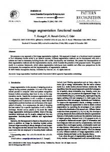
Fig. 1. Best-first branch-and-bound optimization on the tree of nested regions finds the globally-optimal ω by the top-down propagation of the active front (see text for details). At the moment when the lowest lower bound of the front is observed at leaf node, the process terminates with the global minimum found without traversing the whole tree.

In addition to the best-first branch-and-bound search we also tried the depthfirst branch-and-bound [8]. When problem-specific heuristics are available that give good initial solutions, this variant may lead to moderate (up to a factor of 2) time savings. Interestingly, the depth-first variant of the search, which maintains upper bounds on the global optimum, may benefit significantly from the use of flow bounds discussed above. Nevertheless, we stick with the best-first branch-and-bound for the final experiments due to its generality (no need for initialization heuristics). In the rest of the paper we detail how the general framework developed above may be used within different segmentation scenarios.

4 4.1

Segmentation with Shape Priors Constructing Shape Prior

We start with the segmentation with shape priors. The success of such segmentation crucially depends on the way shape prior is defined. Earlier works have often defined this prior as a Gaussian distribution of some geometrical shape statistics (e.g. control point positions or level set functions) [29, 24]. In reality, however, pose variance and deformations specific to the object of interest lead to highly non-Gaussian, multi-modal prior distributions. For better modeling of prior distributions, [9] suggested the use of non-parametric kernel densities. Our approach to shape modeling is similar in spirit, as it also uses exemplarbased prior. Arguably, it is more direct, since it involves the distances between the binary segmentations themselves, rather than their level set functions. Our approach to shape modeling is also closely related to [15] that used shape hierarchies to detect or track objects in image edge maps. We assume that the prior is defined by the set of exemplar binary segmentations {yω |ω ∈ Ω}, where Ω is a discrete set indexing the exemplar segmentations.

8

Extended technical report of ECCV-2008 publication

Then the following term introduces a joint prior over the segmentation and the non-local parameter into the segmentation process: X X Eprior (x, ω) = ρ(x, yω ) = (1 − ypω )·xp + ypω ·(1 − xp ) , (3) p∈V

p∈V

where ρ denotes the Hamming distance between segmentations. This term clearly has the form (1) and therefore its combinations with other terms of this form can be optimized within our framework. Being optimized over the domain 2V ⊗ Ω, this term would encourage the segmentation x to be close in the Hamming distance to some of the exemplar shapes. Note, that the Hamming distance in the continuous limit may be interpreted as the L1-distance between shapes. It is relatively straightforward to modify the term (3) to replace the Hamming distance with discrete approximations of other distances (L2, truncated L1 or L2, data-driven Mahalonobis distance, etc.). The full segmentation energy then may be defined by adding a standard contrast-sensitive edge term [3]: ||Kp −Kq ||

Eshape (x, ω) = Eprior (x, ω) +

X p,q∈E

λ

σ e− |p − q|

·|xp − xq | ,

(4)

where ||Kp − Kq || denote the SAD (L1) distance between RGB colors of the pixels p and q in the image (λ and σ were fixed throughout the experiments described in this section), |p − q| denotes the distance between the centers of the √ pixels p and q (being either 1 or 2 for the 8-connected grid). The functional (4) thus incorporates the shape prior with edge-contrast cues. In practice, the set Ωshape could be huge, e.g. tens of millions exemplars. Therefore, representation and hierarchical clustering of the exemplar segmentations y ω , ω ∈ Ω may be challenging. In addition, the aggregated potentials for each node of the tree should be precomputed and stored in memory. Fortunately, this is accomplishable in many cases when the translation invariance is exploited. In more detail, the set Ωshape is factorized it into the Cartesian product of two sets Ωshape = ∆ ⊗ Θ. The factor set ∆ indexes the set of all exemplar segmentations yδ centered at the origin (this set would typically correspond to the variations in scale, orientation as well as non-rigid deformations). The factor set Θ then corresponds to the shift transformations and ensures the translation invariance of the prior. Any exemplar segmentation yω , ω = δ ⊗ θ is then defined as some exemplar segmentation yδ centered at the origin and then shifted by the shift θ. Being much smaller than Ωshape , both factor sets can be clustered in hierarchy trees. For the factor set ∆ we used agglomerative clustering (a complete linkeage algorithm that uses the Hamming distance between the exemplar segmentations). The factor set Θ uses the natural hierarchical clustering of the quad-tree. Then the tree over Ωshape is defined as a “product” of the two factor trees (we omit the details about the particular implementation). The aggregated potentials FΩ and BΩ in (2) for tree nodes are precomputed in a bottom-up

Extended technical report of ECCV-2008 publication

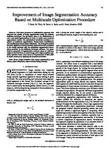
Exemplars yω

Non-local shape prior+Edge cues

9

Intensity+Edge cues

Fig. 2. Using the shape prior constructed from the set of exemplars (left column) our approach can accomplish segmentation of an object undergoing general 3D pose changes within two differently illuminated sequences (two middle columns). Note the varying topology of the segmentations. For comparison, we give the results of a standard graph cut segmentation (right column): even with parameters tuned specifically to the test images, separation is entirely inaccurate.

pass and stored in memory. The redundancy arising from translation invariance is used to keep the required amount of memory reasonable. Note the three properties of our approach to segmentation with shape priors. Firstly, since any shapes can be included in Ωshape , general 3D pose transformations and deformations may be handled. Secondly, the segmentations may have general varying topology not restricted to segments with single-connected boundaries. Thirdly, our framework is general enough to introduce other terms in the segmentation process (e.g. regional terms used in a standard graph cut segmentation [3]). These properties of our approach are demonstrated within the following experiments.

4.2

Experiments

Single object+3D pose changes. In our first experiment, we constructed a shape prior for a single object (a coffee cup) undergoing 3D pose changes. We obtained a set of outlines using “blue-screening”. We then normalized these outlines (by centering at the origin, resizing to a unit scale and orienting the principle axes with the coordinate axes). After that we clustered the normalized outlines using k-means. A representative of each cluster was then taken into the exemplar set. After that we added scale variations, in-plane rotations, and translations. As a result, we got a set {yω |ω ∈ Ωshape } containing about 30,000,000 exemplar shapes(while the set ∆ contained about 1900 shapes).

10

Extended technical report of ECCV-2008 publication

Fig. 3. Results of the global optimization of (5) on some of the 170 UIUC car images including 1 of the 2 cases where localization failed (bottom left). In the case of the bottom right image, the global minimum of (4) (yellow) and the result of our feature-based car detector (blue) gave erroneous localization, while the global minimum of their combination (5) (red) represented an accurate segmentation.

The results of the global optimization of the functional (4) for the frames from the two sequences containing clutter and camouflage are shown in Fig. 2. On average, we observed that segmenting 312x272 image took about 30 seconds of an Intel-2.40 GHz CPU and less than 1 Gb of RAM. The proportion of the nodes of the tree traversed by the active front was on average about 1 : 5000. Thus, branch-and-bound tree search used in our framework improved very considerably over exhaustive search, which would have to traverse all leaves (1 : 2 of the tree). As a baseline algorithm, we considered the segmentation with a “standard” graph cut functional, replacing non-local shape prior term with a local intensityP based term p∈V (I − Ip )·xp , adjusting the constant I for each frame so that it gives the best results. However, since the intensity distributions of the cup and the backgrounds overlapped significantly, the segmentations were grossly erroneous (Fig. 2 – right column). Object class+translation invariance. In the second experiment, we performed the segmentation with shape priors on UIUC car dataset (the version without scale variations), containing 170 images with cars in uncontrolled environment (city streets). The prior set ∆ was built by manual segmentation of 60 training images coming with the dataset. The set of shifts Θ was defined by the varying size of test images. While the test image sizes varyied from 110x75 to 360x176, the size of Ωshape varied from 18,666 to 2,132,865. We computed the globally optimal segmentations under the constructed prior using the energy (4). Using the bounding boxes of the cars provided with the dataset, we found that in 6.5% of the images the global minima corresponded to clutter rather than cars. To provide a baseline for localization accuracy based on edge cues and a

Extended technical report of ECCV-2008 publication

11

set of shape templates, we considered Chamfer matching (as e.g. in [15]). For the comparison we used the same set of templates, which were matched against truncated Canny-based chamfer distance (with optimally tuned truncation and Canny sensitivity parameters). In this way, the optimal localization failed (i.e. corresponded to clutter rather than a car) in 12.4% of the images. Clearly, segmenting images using (4) takes into account the shape prior and edge-contrast cues, but ignores the appearance typical for the object category under consideration. At the same time, there exists a large number of algorithms working with image appearance cues and performing object detection based on these cues (see e.g. [23] and references therein). Typically, such algorithms produce the likelihood of the object presence either as a a function of a bounding box or even in the form of per-pixel “soft segmentation” masks. Both types of the outputs can be added into the functional (1) either via constant potential C(Ω) or via unary potentials. In this way, such appearance-based detectors can be integrated with shape prior and edge-contrast cues. As an example of such integration, we devised a simple detector similar in spirit to [23]. The detector looked for the appearance features typical for cars (wheels) using normalized cross-correlation. Each pixel in the image then “voted” for the location of the car center depending on the strength of the response to the detector and the relative position of the wheels with respect to the car center observed on the training dataset. We then added an additional term Cvote (ω) in our energy (1) that for each ω equaled minus the accumulated strength of the votes for the center of yω : ||Kp −Kq ||

Eshape&detect (x, ω) = Cvote (ω) + Eprior (x, ω) +

X p,q∈E

λ

σ e− |p − q|

·|xp − xq | , (5)

Adding the appearance-based term improved the robustness of the segmentation, as the global optima of (5) corresponded to clutter only in 1.2% of the images. The global minima found for some of the images are shown in Fig. 3. Note, that for our simple detector on its own the most probable bounding box corresponded to clutter on as much as 14.7% of the images. In terms of the performance, on average, for the functional (5) the segmentation took 1.8 seconds and the proportion of the tree traversed by the active front was 1 : 441. For the functional (4), the segmentation took 6.6 seconds and the proportion of the tree traversed by the active front was 1 : 131. This difference in performance is natural to branch-and-bound methods: the more difficult and ambiguous is the optimization problem, the larger is the portion of the tree that has to be investigated.

5

Segmentation with Color/Intensity Priors

Our framework can also be used to impose non-local priors on the intensity or color distributions of the foreground and background segments, as the examples below demonstrate.

12

5.1

Extended technical report of ECCV-2008 publication

Segmenting Grayscale Images: Chan-Vese Functional

183x162, time=3s, 300x250, time=4s, proportion=1:115 proportion=1:103

385x264, time=16s, proportion=1:56

371x255, time=21s, proportion=1:98

Fig. 4. The global minima of the Chan-Vese functional for medical and aerial images. These global minima were found using our framework in the specified amount of time; specified proportion of the tree was traversed.

In [7] Chan and Vese have proposed the following popular functional for the variational image segmentation problem: E(S, cf , cb ) = µ

Z

Z dl + ν

∂S

dp + λ1 S

Z 

I(p) − cf

S

2

dp + λ2

Z 

I(p) − cb

2

dp ,

¯ S

(6) where S denotes the foreground segment, and I(p) is a grayscale image. The first two terms measure the length of the boundary and the area, the third and the forth terms are the integrals over the fore- and background of the difference between image intensity and the two intensity values cf and cb , which correspond to the average intensities of the respective regions. Traditionally, this functional is optimized using level set framework [25]converging to one of its local minima. Below, we show that the discretized version of this functional can be optimized globally within our framework. Indeed, the discrete version of (6) can be written as (using notation as before): µ ·|xp − xq |+ |p − q| p,q∈E  2 X X  ν + λ1 (I(p) − cf )2 ·xp + λ2 I(p) − cb ·(1 − xp ) .

E(x, (cf , cb )) =

p∈V

X

(7)

p∈V

Here, the first term approximates the first term of (6) (the accuracy of the approximation depends on the size of the pixel neighborhood [4]), and the last two terms express the last three terms of (6) in a discrete setting. The functional (7) clearly has the form (1) with non-local parameter ω = {cf , cb }. Discretizing intensities cf and cb into 255 levels and building a quadtree over their joint domain, we can apply our framework to find the global minima of (6). Example globally optimal segmentations are shown on Fig. 4.

Extended technical report of ECCV-2008 publication

5.2

13

Segmenting Color Images: GrabCut functional

In [26], the GrabCut framework for the interactive color image segmentation based on Gaussian mixtures was proposed. In GrabCut, the segmentation is driven by the following energy: X EGrabCut (x, (GM f , GM b )) = − log(P(Kp | GM f ))·xp + p∈V

(8)

||K −Kq ||2

+

X p∈V

X λ1 + λ2 ·e− p β b − log(P(Kp | GM ))·(1 − xp )+ |p − q|

·|xp − xq | .

p,q∈E

Here, GM f and GM b are Gaussian mixtures in RGB color space and the first two terms of the energy measure how well these mixtures explain colors Kp of pixels attributed to fore- and background respectively. The third term is the contrast sensitive edge term, ensuring that the segmentation boundary is compact and tends to stick to color region boundaries in the image. In addition to this energy, the user provides supervision in the form of a bounding rectangle and brush strokes, specifying which parts of the image should be attributed to the foreground and to the background. The original method [26] minimizes the energy within EM-style process, alternating between (i) the minimization of (8) over x given GM f and GM b and (ii) refitting the mixtures GM f and GM b given x. Despite the use of the global graph cut optimization within the segmentation update step, the whole process yields only a local minimum of (8). In [26], the segmentation is initialized to the provided bounding box and then typically shrinks to one of the local minima. The energy (8) has the form (1) and therefore can be optimized within Branch-and-Mincut framework, provided that the space of non-local parameters (which in this case is the joint space of the Gaussian mixtures for the foreground and for the background) is discretized and the tree of the subregions is built. In this scenario, however, the dense discretization of the non-local parameter space is infeasible (if the mixtures contain n Gaussians then the space is described by 20n − 2 continuous parameters). It is possible, nevertheless, to choose a much smaller discrete subset Ω that is still likely to contain a good approximation to the globally-optimal mixtures. To construct such Ω, we fit a mixture of M = 8 Gaussians G1 , G2 , ...GM with the support areas a1 , a2 , ...aM to the whole image. The support area ai here counts the number of pixels p such as ∀j P(Kp |Gi ) ≥ P(Kp |Gj ). We assume that the components are ordered such that the support areas decrease (ai > ai+1 ). Then, the Gaussian mixtures we consider are defined by the binary vector β = {β1 , β2 . . . βM } ∈ {0, 1}M specifying which Gaussians should be included into P P the mixture: P(K| GM (β)) = i βi ai P(K|Gi ) / i βi ai . The overall set Ω is then defined as {0, 1}2M , where odd bits correspond to the foreground mixture vector β f and even bits correspond to the background mixture vector β b . Vectors with all even bits and/or all odd bits equal to zero do not correspond to meaningful mixtures and are therefore assigned an infinite

14

Extended technical report of ECCV-2008 publication

cost. The hierarchy tree is naturally defined by the bit-ordering (the first bit corresponding to subdivision into the first two branches etc.).

Image+input

GrabCut[26](−618) Branch&Mincut(−624) Combined(−628)

Image+input

GrabCut[26](−593) Branch&Mincut(−584) Combined(−607)

Fig. 5. Being initialized with the user-provided bounding rectangle (shown in green in the first column) as suggested in [26], EM-style process [26] converges to a local minimum (the second column). Branch-and-Mincut result (the third column) escapes that local minimum and after EM-style improvement lead to the solution with much smaller energy and better segmentation accuracy (the forth column). Energy values are shown in brackets.

Depending on the image and the value of M , the solutions found by Branchand-Mincut framework may have larger or smaller energy (8) than the solutions found by the original EM-style method [26]. This is because Branch-and-Mincut here finds the global optimum over the subset of the domain of (8) while [26] searches locally but within the continuous domain. However, for all 15 images in our experiments, improving Branch-and-Mincut solutions with a few EM-style iterations [26] gave lower energy than the original solution of [26]. In most cases, these additional iterations simply refit the Gaussians properly and change very few pixels near boundary (see Fig. 5). In terms of performance, for M = 8 the segmentation takes on average a few dozen seconds (10s and 40s for the images in Fig. 5) for 300x225 image. The proportion of the tree traversed by an active front is one to several hundred (1:963 and 1:283 for the images in Fig. 5). This experiment suggests the usefulness of Branch-and-Mincut framework as a mean of obtaining good initial point for local methods, when the domain space is too large for an exact branch-and-bound search.

Extended technical report of ECCV-2008 publication

6

15

Conclusion

The Branch-and-Mincut framework presented in this paper finds global optima of a wide class of energies dependent on the image segmentation mask and nonlocal parameters. The joint use of branch-and-bound and graph cut allows efficient traversal of the solution space. The developed framework is useful within a variety of image segmentation scenarios, including segmentation with non-local shape priors and non-local color/intensity priors. Future work includes the extension of Branch-and-Mincut to other problems, such as simultaneous stitching and registration of images, as well as deriving analogous branch-and-bound frameworks for combinatorial methods other than binary graph cut, such as minimum ratio cycles and multilabel MRF inference.

7

Acknowledgements

We would like to acknowledge discussions and feedback from Vladimir Kolmogorov and Pushmeet Kohli. Vladimir has also kindly made several modifications of his code of [5] that allowed to reuse network flows more efficiently.

References 1. S. Agarwal, M. Chandaker, F. Kahl, D. Kriegman, S. Belongie: Practical Global Optimization for Multiview Geometry. In ECCV 2006. 2. E. Boros, P. Hammer: Pseudo-boolean optimization. Discrete Applied Mathematics, 123(1-3), 2002. 3. Y. Boykov, M.-P. Jolly: Interactive Graph Cuts for Optimal Boundary and Region Segmentation of Objects in N-D Images. In ICCV 2001. 4. Y. Boykov, V. Kolmogorov: Computing Geodesics and Minimal Surfaces via Graph Cuts. In ICCV 2003. 5. Y. Boykov, V. Kolmogorov: An Experimental Comparison of Min-Cut/Max-Flow Algorithms for Energy Minimization in Vision. In PAMI, 26(9), 2004. 6. M. Bray, P. Kohli, Philip Torr: PoseCut: Simultaneous Segmentation and 3D Pose Estimation of Humans Using Dynamic Graph-Cuts. In ECCV 2006. 7. T. Chan, L. Vese: Active contours without edges. Trans. Image Process., 10(2), 2001. 8. J. Clausen: Branch and Bound Algorithms - Principles and Examples. Parallel Computing in Optimization (1997). 9. D. Cremers, S. Osher, S. Soatto: Kernel Density Estimation and Intrinsic Alignment for Shape Priors in Level Set Segmentation. IJCV 69(3), 2006. 10. D. Cremers, F. Schmidt, F. Barthel: Shape Priors in Variational Image Segmentation: Convexity, Lipschitz Continuity and Globally Optimal Solutions. In CVPR 2008. 11. D. Greig, B. Porteous, A. Seheult: Exact maximum a posteriori estimation for binary images. Journal of the Royal Statistical Society, 51(2), 1989. 12. P. Felzenszwalb: Representation and Detection of Deformable Shapes. PAMI 27(2), 2005. 13. D. Freedman: Effective tracking through tree-search. PAMI, 25(5), 2003.

16

Extended technical report of ECCV-2008 publication

14. D. Freedman, T. Zhang: Interactive Graph Cut Based Segmentation with Shape Priors. In CVPR 2005. 15. D. Gavrila, V. Philomin: Real-Time Object Detection for ”Smart” Vehicles. In ICCV 1999. 16. R. Huang, V. Pavlovic, D. Metaxas: A graphical model framework for coupling MRFs and deformable models. In CVPR 2004. 17. J. Kim, R. Zabih: A Segmentation Algorithm for Contrast-Enhanced Images. ICCV 2003. 18. P. Kohli, P. Torr: Effciently Solving Dynamic Markov Random Fields Using Graph Cuts. In ICCV 2005. 19. V. Kolmogorov, R. Zabih: What Energy Functions Can Be Minimized via Graph Cuts? In ECCV 2002. 20. V. Kolmogorov, Y. Boykov, C. Rother: Applications of Parametric Maxflow in Computer Vision. In ICCV 2007. 21. M. Pawan Kumar, P. Torr, A. Zisserman: OBJ CUT. In CVPR 2005. 22. C. Lampert, M. Blaschko, T. Hofman. Beyond Sliding Windows: Object Localization by Efficient Subwindow Search. In CVPR 2008. 23. B. Leibe, A. Leonardis, B. Schiele: Robust Object Detection with Interleaved Categorization and Segmentation. IJCV 77(3), 2008. 24. M. Leventon, E. Grimson, O. Faugeras: Statistical Shape Influence in Geodesic Active Contours. In CVPR 2000. 25. S. Osher, J. Sethian: Fronts Propagating with Curvature Dependent Speed: Algorithms Based on Hamilton-Jacobi Formulations. J. of Comp. Phys., 79(8), 1988. 26. C. Rother, V. Kolmogorov, A. Blake: ”GrabCut”: interactive foreground extraction using iterated graph cuts. ACM Trans. Graph. 23(3), 2004. 27. T. Schoenemann, D. Cremers: Globally Optimal Image Segmentation with an Elastic Shape Prior. In ICCV 2007. 28. A. Kemal Sinop, L. Grady: Uninitialized, Globally Optimal, Graph-Based Rectilinear Shape Segmentation - The Opposing Metrics Method. In ICCV 2007. 29. Y. Wang, L. Staib: Boundary Finding with Correspondence Using Statistical Shape Models. In CVPR 1998.

Appendix: Proof of the monotonicity of the lower bound By definition (see (2) in section 3.2), our bound L(Ω) equals  L(Ω) = min min C(ω) + x∈2V

ω∈Ω

X p∈V

min F p (ω)·xp +

ω∈Ω

 X p∈V

min B p (ω)·(1 − xp ) +

ω∈Ω

X p,q∈E

min P pq (ω)·|xp − xq | ,

ω∈Ω

(9)

where x ∈ 2V is the segmentation vector, V is the set of pixels, ω is the non-local parameter, C, F p , B p , P pq are real-valued functions of ω. We need to prove that if Ω1 ⊂ Ω2 then L(Ω1 ) ≥ L(Ω2 ) (monotonicity).

Extended technical report of ECCV-2008 publication

17

Proof. Let us denote with A(x, Ω) the expression within the outer minimum of (9):  X A(x, Ω) = min C(ω) + min F p (ω)·xp + ω∈Ω

p∈V

ω∈Ω

 X p∈V

min B p (ω)·(1 − xp ) +

ω∈Ω

X p,q∈E

min P pq (ω)·|xp − xq | .

ω∈Ω

(10)

Then, (9) reformulates as: L(Ω) = min A(x, Ω) . x∈2V

(11)

Assume Ω1 ⊂ Ω2 . Let us prove that for any fixed x, for all pixels p and edges pq, the following holds: min C(ω) ≥ min C(ω)

(12)

min F (ω)·xp ≥ min F p (ω)·xp

(13)

min B (ω)·(1 − xp ) ≥ min B p (ω)·(1 − xp )

(14)

min P pq (ω)·|xp − xq | ≥ min P pq (ω)·|xp − xq |.

(15)

ω∈Ω1 p

ω∈Ω1 p

ω∈Ω1

ω∈Ω2

ω∈Ω2

ω∈Ω2

ω∈Ω1

ω∈Ω2

This is because, firstly, all values xp , 1 − xp , and |xp − xq | are non-negative (recall that all xp takes the value of 0 or 1) and, secondly, all minima on the left sides are taken over a subset of the domain of the same minima on the left sides. Consider for instance (15) for some edge pq. If |xp −xq | = 0 then (15) is trivial (0 ≥ 0). Otherwise (if |xp − xq | = 1) (15) is eqivalent to minω∈Ω1 P pq (ω) ≥ minω∈Ω2 P pq (ω), which is true because the domain on the left lies inside the domain on the right (Ω1 ⊂ Ω2 by assumption). Same argument holds for all inequalities (12)–(15). Summing up inequalities (12)–(15) over all pixels p and edges pq and taking into account the definition (10), we get: ∀x

A(x, Ω1 ) ≥ A(x, Ω2 ) .

(16)

I.e. monotonicity holds for any fixed x. Let x1 be the segmentation delivering the global optimum of A(x, Ω1 ): x1 = argminx∈2V A(x, Ω1 ). Let x2 be the segmentation delivering the global optimum of A(x, Ω2 ): x2 = argminx∈2V A(x, Ω2 ). Then, L(Ω1 ) = A(x1 , Ω1 ) ≥ A(x1 , Ω2 ) ≥ A(x2 , Ω2 ) = L(Ω2 ) .

(17)

18

Extended technical report of ECCV-2008 publication

Here, the first equality is by the definition of L, A, x1 (see (11)); the following inequality follows from (16); the next inequality is by the definition of x2 ; the last equality is by the definition of L, A, x2 (see (11)). Therefore: L(Ω1 ) ≥ L(Ω2 ) .