Fast Semi-Supervised Image Segmentation by ... - Semantic Scholar

FAST SEMI-SUPERVISED IMAGE SEGMENTATION BY NOVELTY SELECTION Ant´onio R. C. Paiva1 and Tolga Tasdizen1,2 1

2

Scientific Computing and Imaging Institute Department of Electrical and Computer Engineering University of Utah, Salt Lake City, UT 84112, USA

ABSTRACT The goal of semi-supervised image segmentation is to obtain the segmentation from a partially labeled image. By utilizing the image manifold structure in labeled and unlabeled pixels, semi-supervised methods propagate the user labeling to the unlabeled data, thus minimizing the need for user labeling. Several semi-supervised learning methods have been proposed in the literature. Although results have been promising, these methods are very computationally intensive. In this paper, we propose novelty selection as a pre-processing step to reduce the number of data points while retaining the fundamental structure of the data. Since the computational complexity is a power of the number of points, it is possible to significantly reduce the overall computation requirements. Results in several images show that the computation time is greatly reduced without sacrifice in segmentation accuracy. Index Terms— Semi-supervised segmentation, image segmentation, novelty selection. 1. INTRODUCTION Image segmentation is a challenging task and remains an open problem in image processing. Unsupervised methods explore the intrinsic data structure to segment the image into regions with different statistics. However, these methods often fail to achieve the desired result, especially if the desired segmentation includes regions with very different characteristics. On the other extreme, supervised image segmentation methods first learn a classifier from a labeled training set. Although these methods are likely to perform better, marking the training set is very time consuming. Semi-supervised image segmentation methods circumvent these problems by inferring the segmentation from partially labeled images. The key difference from supervised learning is that semisupervised methods utilize the data structure in both the labeled and unlabeled data points [1]. Hence, the main advantage of semi-supervised image segmentation methods is This work was supported in part by the NIH, National Institute of Biomedical Imaging and Bioengineering, under grant RO1EB005832.

that they take advantage of the user markings to direct the segmentation, while minimizing the need for user labeling. There are several general approaches towards semisupervised learning, but recent developments have focused on graph-based methods [1], likely because the graph-based representation naturally copes with nonlinear data manifolds. In this formulation, data points are represented by nodes in a graph, and the edge weights are given by some measure of distance or affinity between the data points. Then, the labels for the unlabeled points are found by propagating the labels of labeled points through the graph. Based on this methodology, a number of methods have been proposed [2, 3, 4, 5, 6], differing mainly on the way how the edge weights are defined and/or how to propagate the labels (see, for example, [7, 1] for comprehensive reviews). Although results from graphbased semi-supervised methods have been promising, these methods are severely limited by the number of data points. This is because label propagation in the graph requires first the computation of the connectivity matrix for all the data, and then the labels are propagated using this matrix. Consequently, the computational complexity grows exponentially with the number of points. This severely limits the application of semi-supervised learning methods for image segmentation because, even for relatively small images, one can easily have tens of thousands of pixels. To mitigate the computational burden of semi-supervised learning methods, we propose the use of novelty selection as a pre-processing step. Given the data (labeled and unlabeled points), novelty selection finds a reduced set of points while preserving the overall structure of the data. By applying semi-supervised learning on this “representative set,” one greatly reduces the computational complexity and storage requirements. The final segmentation can then be achieved by extending the labeling of the points in the representative set to their nearest neighbors. 2. NOVELTY SELECTION Novelty selection is closely related to Platt’s work on resourceallocating networks [8]. Platt introduced a criterion to decide whether a given input point should be added to a growing

radial basis function neural network in order to minimize network error. The point was added if the distance to the other points already in the network was larger than a threshold, and the network error was above another threshold. Basically, Platt’s criterion aims to achieve a small error with the least possible number of reference points added to the network. Implicitly, small error requires an accurate representation of the input data space, but the key observation is that nearby points in the input space convey approximately the same information and, therefore, they can be replaced by a single representative point with minimal loss. The same observation applies in our case. For semisupervised learning, we want to accurately reflect the data structure with the smallest number of reference points. This can be achieved by adding a data point to the set of representative points only if the smallest distance to all other points in the representative set is larger than a threshold δ. In other words, a point is selected if it provides novel information about the data space, hence the name novelty selection. Thus, our method ensures that enough data points are kept to completely cover the space while keeping the number of points needed to achieve this covering to a minimum. Hence, data points closer to a representative point than δ do not need to be considered during semi-supervised learning (only the representative set is used), which makes the propagation of labels much faster. In a sense, these ideas are also similar to those of vector quantization [9]. Indeed, vector quantization could be utilized instead of novelty selection. However, a key difference is that novelty selection aims only to preserve the overall space covering, without explicitly attempting to model the density of the data. For this reason, and as required towards a fast solution, novelty selection is computationally much faster than vector quantization (even when compared to k-means), because the representative set can be obtained in a single-pass through the data. Another fundamental advantage is that there is no need to select a priori the number of representative points. The novelty selection criterion simply adds points to the representative set until no points verify the criterion. Since information is lost during novelty selection (due to the reduction of the number of points), care must be taken to ensure that essential information for semi-supervised learning is preserved. Central to many semi-supervised learning methods is the smoothness assumption, meaning that nearby points in a dense region are likely to have the same label. A corollary is that points with different labels should be separated by regions with low density. Consequently, novelty selection must preserve the differences in density between a region with the same label and the separation to other regions. In novelty selection, this is ensured by making δ small compared to the distance between points with different labels. Clearly, the optimal value of δ represents a trade-off between the reduction of the number of points (achieved by increasing δ), and the preservation of differences in density (by decreasing δ).

2.1. Algorithm The algorithm for novelty selection and the procedure for its use in semi-supervised image segmentation is now summarized. Consider a set of N data points X = {x1 , . . . , xN }, and denote the representative set by Y . In addition, denote by IY the set of indices of points in X included in Y , and IX = {j1 , . . . , jN } the set of indices of the nearest neighbor in Y for each xi ∈ X. Then, novelty selection proceed as follows: • Initialize Y = {x1 }, IY = {1} and IX = {1}; • For each xi ∈ X, – Compute d(xi , Y ), the vector of distances of xi to all elements in Y ; – If min(d(xi , Y )) > δ, Add xi to Y , and set ji = i, else, Set ji = arg minn d(xi , yn ), yn ∈ Y . It must be noted that, strictly speaking, the index sets IY , IX are not used for novelty selection, but to retain information that is needed to compute the semi-supervised image segmentation result. Also, if necessary, the algorithm can be modified to operate incrementally simply by initializing the set Y with the available representative set instead (and setting IY and IX accordingly). To obtain the final result, the novelty selection algorithm has to be integrated in the semi-supervised framework. The two main differences are the use of novelty selection as a preprocessing step, and the assignment of the labels obtained from semi-supervised learning to the remaining unlabeled points. Summarizing, the segmentation is obtained with: 1. Apply novelty selection to all the data; 2. In addition to the representative set, ensure all labeled data points are included in the analysis; 3. Propagate labels through semi-supervised learning; 4. Label the remaining unlabeled points (not included in the analysis with semi-supervised learning) with the label of their nearest neighbor in the representative set. Note that step 2 is not required for the analysis but is recommended since, in this way, one makes sure to use all the information available from user labeling. The index sets IY and IX obtained from novelty selection can be utilized in steps 2 and 4, respectively, avoiding further computations. 3. RESULTS In this section, the ideas described above are demonstrated in some examples. First, we illustrate semi-supervised segmentation and novelty selection in a simple manifold classification example. Then, the new proposed approach is demonstrated for semi-supervised image segmentation.

1.5

1.5

1

1

0.5

0.5

0

0

−0.5

−0.5

−1

−1

−1.5 −2

−1.5 −2

−1.5

−1

−0.5

0

0.5

1

1.5

2

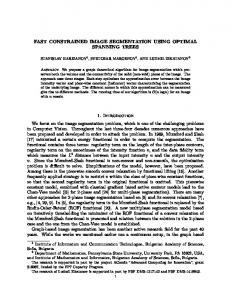
(a) Data with two labeled points. 1.5

−1

−0.5

0

0.5

1

1.5

2

1.5

1

1

0.5

0.5

0

0

−0.5

−0.5

−1

−1

−1.5 −2

−1.5

(b) Label propagation on all the data.

also yields the desired result, as shown in Fig. 1(d) (representative points are show with light face color). Notice that the kernel size was increased in the second case, since the data appears more “spaced out” due to novelty selection. Understandably, the kernel size was chosen to be higher than δ, since novelty selection ensures that the minimum distance between neighbors is greater than δ. For comparison, the computation times are provided: label propagation on the whole dataset takes 0.22 seconds, whereas using novelty selection the whole process takes only 0.01 seconds.

−1.5

−1

−0.5

0

0.5

1

1.5

2

(c) Representative set from novelty selection.

−1.5 −2

3.2. Image segmentation

−1.5

−1

−0.5

0

0.5

1

1.5

2

(d) Final label assignment, with label propagation on the representative set.

Fig. 1: Illustration of novelty selection and semi-supervised learning on the “two moons” dataset. For the experiments, with or without novelty selection, the semi-supervised learning algorithm proposed by Zhou et al. [2] was utilized. In this method, label propagation is implemented by solving the equation, f = (I − αS)−1 Y,

(1)

where I is the identity matrix, S is the normalized affinity 1 1 matrix given by S = D− 2 W D− 2 , and Y is the vector with the available labeling (entries in Y are set to −1/ + 1 for labeled points, and zero for unlabeled points). For simplicity, we consider only the two-class problem here, but the approach can be easily extended to any number of classes if needed (see [2] for details). The matrix W is defined by Wij = exp(−kxi − xj k2 /2σ 2 ) if i 6= j and Wii = 0, and D is a diagonal matrix with the ith diagonal entry equal to the sum of the ith row of W . All experiments were performed in Matlab using sparse matrix computation for efficiency. 3.1. Manifold classification In this example we utilize the “two moons” dataset shown in Fig. 1 to illustrate the use of novelty selection for semisupervised learning. Propagating the labels using kernel size σ = 0.1 and α = 0.99 (from [2]), one obtains the desired result shown in Fig. 1(b). If novelty selection is applied to the dataset with δ = 0.2, the number of points is reduced from 500 to 52, marked in Fig. 1(c). Then, performing label propagation on these representative points with σ = 0.25 and α = 0.99, and assigning the labels to the remaining points

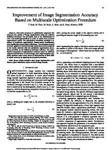
We now provide results of applying novelty selection for semi-supervised image segmentation. In our experiments, the feature vector for each pixel was chosen to be a 5 × 5 image patch centered at the pixel, and over the three color components, resulting in a 75-dimensional feature vector. With our image intensity values normalized to the interval [0, 1], the threshold for novelty selection was set to δ = 0.5. It was found empirically that this value of δ yielded a good compromise in reduction of the number of points and improvement in computation speed, without noticeable detriment in segmentation accuracy. α was set to 0.1. The kernel size σ was set to 1 when novelty selection was utilized, and 0.1 for computation with all the data. It is important to note that we attempted to further reduce the kernel size when computing with all the data to try to increase the sparsity of the matrices and thus speed the computation, but it was found that 0.1 was the smallest kernel size that would reliably yield the correct segmentation. The results of semi-supervised image segmentation using novelty selection are given in Fig. 2. The segmentation of the first two images illustrates a situation where the desired segmentation would be very hard to obtain using unsupervised segmentation methods, but is obtained readily through semisupervision thanks to the user labeling. To compare the computation time, we computed the segmentation of the images in Fig. 2 with and without novelty selection. The same user labeling was utilized in both cases. The results are presented in Table 1. From these results, the improvement in computation speed by using novelty selection is clearly noticeable. 4. CONCLUSIONS In this paper, novelty selection is proposed as a pre-processing method to reduce the computational requirements of semisupervised methods. The fundamental assumption is that neighboring points in the features space convey approximately the same information, and these can be represented by one representative point without loss in the information. Indeed, as discussed in section 2 and shown in the results, if the radius of the neighborhood is chosen carefully, there is

no noticeable decrease in accuracy. And, most importantly, because of the smaller number of points in the representative set, label propagation can be made much faster. Novelty selection was applied here for semi-supervised image segmentation. However, the concept is directly applicable to other applications using semi-supervised learning, as should be clear from our exposition. Likewise, note that novelty selection is not tied to any specific semi-supervised learning method and other graph-based semi-supervised methods could be used. For this work, the selection of the novelty selection parameter δ was done empirically. Future work may focus on determining its value automatically. Although crossvalidation techniques may potentially be utilized, this is not straightforward due to nature of semi-supervised learning and the small number of labeled points. 5. REFERENCES [1] Olivier Chapelle, Bernhard Sch¨olkopf, and Alexander Zien, Eds., Semi-Supervised Learning, MIT Press, 2006. [2] Dengyong Zhou, Olivier Bousquet, Thomas N. Lal, Jason Weston, and Bernhard Sch¨olkopf, “Learning with local and global consistency,” in Advances Neural Information Processing Systems, Vancouver, BC, Canada, Dec. 2003. [3] Fei Wang, Jingdong Wang, Changshui Zhang, and Helen C. Shen, “Semi-supervised classification using linear neighborhood propagation,” in Proc. IEEE Conf. on Computer Vision and Pattern Recognition, New York, NY, USA, June 2006. [4] M. Belkin, P. Niyogi, and V. Sindhwani, “On manifold regularization,” in Proc. Intl. Workshop on Artificial Intelligence and Statistics, Barbados, Jan. 2005. [5] Xiaojin Zhu, Zoubin Ghahramani, and John Lafferty, “Semi-supervised learning with Gaussian fields and harmonic functions,” in Proc. Intl. Conf. on Machine Learning, Washington, D.C, USA, Aug. 2003. Fig. 2: Semi-supervised image segmentation results. (left) Original images with user labeling, shown as green and blue traces, and (right) segmentation using novelty selection. Table 1: Comparison of computation times with and without novelty selection. All times are in seconds.

Image Tree Beach House Tulips

Dimensions (pixels) 110×122 150×150 128×128 300×200

with novelty selection 24.5 4.6 18.2 640.6

without novelty selection 392.1 2857.8 639.4 12351.4

speedup 16× 621× 35× 19×

[6] N. Houhou, X. Bresson, A. Szlam, T. F. Chan, and J.-P. Thiram, “Semi-supervised segmentation based on nonlocal continuous min-cut,” in Proc. of the Intl. Conf. on Scale Space and Variational Methods in Computer Vision, LNCS 5567, Voss, Norway, June 2009. [7] Xiaojin Zhu, “Semi-supervised learning literature survey,” Computer Sciences TR 1530, University of Winconsin–Madison, 2008. [8] John Platt, “A resource-allocating network for function interpolation,” Neural Comp., vol. 3, no. 2, pp. 213–225, 1991. [9] R. O. Duda, P. E. Hart, and David G. Stork, Pattern classification, Wiley Interscience, 2nd edition, 2000.