Image Understanding Software for Hybrid Hardware - CiteSeerX

Charles River Analytics

55 Wheeler Street

Final Report No. R94061

Cambridge, MA 02138 (617) 491-3474

Issued by U.S. Army Missile Command Under Contract No. DAAH01-94-C-R283 ARPA Order 5916 Amdt 69

Image Understanding Software for Hybrid Hardware Magnús S. Snorrason, Harald Ruda Charles River Analytics 55 Wheeler Street Cambridge, MA 02138

6 March 1995

The views, opinions, and findings contained in this report are those of the authors and should not be construed as an official Agency position, policy, or decision, unless so designated by other official documentation.

Sponsored by: Advanced Research Projects Agency (DoD) SSTO Dates of Contract: 6/21/94 - 1/21/95 Short Title of Work: Hybrid Hardware Principal Investigator: Magnús S. Snorrason ([email protected])

R94061


Abstract In this Phase I effort, we designed a hybrid image understanding system consisting of neural network software running on parallel hardware and symbolic processing software running on conventional hardware. Such a hybrid system exploits the inherent parallelism in neural systems without sacrificing the efficiency of symbolic processing on conventional hardware. We used automatic target recognition for laser-radar (LADAR) imagery as a specific image understanding problem to demonstrate algorithm feasibility. We demonstrated that segmentation can be done without neural methods, but we also determined that the Boundary Contour System neural model of low-level vision offers great potential for improved segmentation, and we performed an efficiency analysis on a massively parallel computer. Our research into the feature extraction process demonstrated that both neuromorphic (local receptive field) and standard statistical features are necessary for high recognition rates. Since these features can be computed independently, they map perfectly onto parallel hardware. Object classification is done by a hierarchy of Fuzzy-ARTMAP neural networks that performs recognition at multiple levels of discrimination for each image object. A hierarchical approach to recognition simplifies the task because each classifier has fewer possible outcomes, and it provides a natural mapping onto coarse-grain parallel hardware.

1

R94061


Acknowledgment This work was performed under ARPA contract DAAH01-94-C-R283 with the US Army Missile Command, Redstone Arsenal, Alabama. The authors thank the Technical Monitor, Mr. Bob Johnson, and the ARPA Technical Official, Dr. Oscar Firschein, for their support and direction on this project.

2

R94061


Table of Contents 1. Introduction ..............................................................................................................................9 1.1. Technical Objectives and Approaches ............................................................................10 1.1.1. Choice of IU Applications ..................................................................................10 1.1.2. Choice of IU Tasks .............................................................................................11 1.1.3. Relationship With Companion Phase I Work .....................................................11 1.2. Summary of Results ........................................................................................................12 1.2.1. Segmentation.......................................................................................................12 1.2.2. Feature Extraction ...............................................................................................13 1.2.3. Classification.......................................................................................................13 1.2.4. Hardware Architectures ...................................................................................... 14 1.3. Report Outline .................................................................................................................15 2. ATR as an Example of IU ........................................................................................................16 2.1. Background .....................................................................................................................16 2.2. Pattern Processing Tasks In ATR ...................................................................................17 2.2.1. Sensor Processing ...............................................................................................17 2.2.2. Image Enhancement ............................................................................................18 2.2.3. Object Detection .................................................................................................18 2.2.4. Object Segmentation ...........................................................................................18 2.2.5. Feature Extraction ...............................................................................................19 2.2.6. Classification.......................................................................................................20 2.3. Pattern Processing Methods ............................................................................................20 2.3.1. Image Processing ................................................................................................20 2.3.1.1. Point Processes........................................................................................20 2.3.1.2. Area Processes ........................................................................................21 2.3.1.3. Frame Processes ......................................................................................21 2.3.1.4. Histogram Operations .............................................................................21 2.3.1.5. Geometric Processes ...............................................................................21 2.3.2. Feature Extraction ...............................................................................................22 2.4. Knowledge Based Reasoning Tasks In ATR ..................................................................23 2.4.1. A Priori Knowledge Integration..........................................................................23 2.4.2. Truth Data ...........................................................................................................23 2.4.3. Decision Fusion...................................................................................................24 2.5. Knowledge Based Reasoning Methods...........................................................................24 2.5.1. Expert System Overview ....................................................................................24 2.5.2. Qualitative Process Theory .................................................................................25 2.5.3. Inference and Reasoning Strategies ....................................................................25 2.5.4. Knowledge Bases for ATR .................................................................................26 3. Neural Paradigms for IU ..........................................................................................................27 3.1. Image Segmentation........................................................................................................27 3

R94061


3.2. Feature Extraction ...........................................................................................................30 3.3. Classification...................................................................................................................33 3.3.1. Invariance ...........................................................................................................34 3.3.1.1. Structural Invariance ...............................................................................34 3.3.1.2. Training Based Invariance ......................................................................34 3.3.1.3. Invariant Feature Extraction....................................................................34 3.3.2. Feature Selection .................................................................................................35 3.3.3. Fuzzy-ARTMAP .................................................................................................36 3.3.3.1. The Original Version ..............................................................................37 3.3.3.2. Our Simplified Version ...........................................................................39 3.4. Uniform vs. Space Variant Resolution Sensors ..............................................................41 4. Hardware Options for Neural Networks .................................................................................. 42 4.1. Types of Parallelism........................................................................................................42 4.2. General Purpose Computers............................................................................................44 4.2.1. Single CPU Processing .......................................................................................44 4.2.2. Distributed Processing ........................................................................................44 4.3. Accelerators and Parallel Computers ............................................................................. 45 4.3.1. High Speed Co-processors ..................................................................................45 4.3.2. High Speed Accelerators.....................................................................................45 4.3.3. Coarse Grain Parallel Computers........................................................................ 46 4.3.4. Massively Parallel Computers (Fine Grain Parallelism).....................................47 4.4. Programmable Neurocomputers ..................................................................................... 47 4.5. Custom Neurocomputers.................................................................................................48 4.5.1. Digital VLSI........................................................................................................48 4.5.2. Analog VLSI .......................................................................................................48 4.5.3. Pulse Modulation VLSI ......................................................................................49 4.6. Commercially Available Hardware ................................................................................49 5. Mapping Neural Paradigms to Parallel Hardware ................................................................... 53 5.1. Image Segmentation........................................................................................................53 5.1.1. BCS/FCS and Massively Parallel Machines .......................................................53 5.1.2. BCS/FCS and Coarse Grain Parallel Machines ..................................................55 5.2. Feature Extraction ...........................................................................................................56 5.3. Classification...................................................................................................................58 5.4. Complete IU System .......................................................................................................60 6. Software Development Environments .....................................................................................61 6.1. Khoros .............................................................................................................................61 6.1.1. Khoros 1 ..............................................................................................................62 6.1.2. Khoros 2 ..............................................................................................................62 6.2. RIPPEN ...........................................................................................................................63 6.3. IUE ..................................................................................................................................63

4

R94061


7. ATR Using LADAR Data ........................................................................................................65 7.1. Virtual Views ..................................................................................................................66 7.2. Segmentation...................................................................................................................68 7.2.1. Segmenting Height Data .....................................................................................69 7.2.2. Segmenting Energy Images ................................................................................72 7.3. 3-D Rotational Invariance and Feature Extraction .........................................................74 7.3.1. Rotational Invariance ..........................................................................................74 7.3.2. Feature Extraction ...............................................................................................76 7.4. Classification...................................................................................................................77 7.4.1. Target Detection Results .....................................................................................77 7.4.2. Target Recognition Results .................................................................................78 8. Conclusions ..............................................................................................................................80 8.1. Summary .........................................................................................................................80 8.2. Conclusions .....................................................................................................................80 8.3. Recommendations For Phase II ......................................................................................81 9. References ................................................................................................................................82

5

R94061


List of Figures Figure 2.2-1: Conventional ATR System Architecture ................................................................16 Figure 2.3.2-1: Object Feature Hierarchy ..................................................................................... 21 Figure 3.1-1: The BCS/FCS System .............................................................................................27 Figure 3.1-2: Horizontal Boundary With Gaps (top) and Horizontal Illusory Contour (bottom) 29 Figure 3.2-1: Gabor Functions in 12 Different Orientations ........................................................ 30 Figure 3.2-2: Sampling Grid for Local Features........................................................................... 32 Figure 3.3.3.1-1: Fuzzy-ARTMAP Block Diagram .....................................................................37 Figure 3.3.3.2-1: Simplified Fuzzy-ARTMAP Architecture ........................................................39 Figure 4.1-1: Types of Parallelism................................................................................................42 Figure 5.1.2-1: Coarse Grain Partitioning of BCS........................................................................ 54 Figure 5.2-1: Coarse Grain Partitioning of Feature Extraction..................................................... 56 Figure 5.3-1: Coarse Grain Partitioning of Classification Hierarchy ........................................... 58 Figure 5.4-1: Parallelization of Our IU System ............................................................................59 Figure 7-1: System Level Block Diagram of ATR System for LADAR Data .............................65 Figure 7.1-1: A Vertical Slice (fixed y) Through A Scene With Range Sensor........................... 66 Figure 7.1-2: Histogram Equalized Height-Coded LADAR Image .............................................68 Figure 7.1-3: Virtual Top View ....................................................................................................68 Figure 7.2-1: Block Diagram for Segmentation and Projection to Virtual View ......................... 69 Figure 7.2-1: Height Thresholded Image ......................................................................................71 Figure 7.2-2: Final Segmentation Binary Mask ............................................................................72 Figure 7.2.2-1: Contrast Enhanced LADAR Reflectance Image ..................................................73 Figure 7.2.2-2: Dispersion at Small Scale.....................................................................................73 Figure 7.2.2-3: Dispersion at Large Scale.....................................................................................73 Figure 7.2.2-4: Sum of Dispersion at Two Scales ........................................................................73 Figure 7.3.1-1: Top-View Projected, Segmented, Isolated, and Rotated Height-Coded Objects 75 Figure 7.3.2-2: Segmented, Isolated, Rotated, and Scaled Reflectance Objects ..........................75 Figure 7.4.2-1: Mobile Artillery Unit Resembling a Tank ...........................................................79

6

R94061


List of Tables Table 4.5-1: Types of Neural VLSI ..............................................................................................47 Table 4.6-1: Commercially Available Neural/Parallel Chips .......................................................49 Table 4.6-2: Commercially Available Neural/Parallel Boards ..................................................... 50

7

R94061


Glossary of Abbreviations ART ATR BCS/FCS BP CAC CISC CPU DSP FPU IU LADAR MAC MIMD PE, PN RISC SIMD SISD VLSI

Adaptive Resonance Theory Automatic Target Recognition Boundary-Contour-System/Feature-Contour-System Back Propagation Compare And Accumulate Complex Instruction Set Computer Central Processing Unit Digital Signal Processor Floating Point Unit Image Understanding Laser Radar Multiply And Accumulate Multiple Instruction Multiple Data Processing Element, Processing Node Reduced Instruction Set Computer Single Instruction Multiple Data Single Instruction Single Data Very Large Scale Integration

8

R94061


1. Introduction Image understanding (IU) is the interpretation of visual information—from image segmentation, feature extraction, and classification—combined with contextual information from ancillary sources such as maps, intelligence, time of day, season, and weather. A common use for IU is in automatic target recognition (ATR), which is defined as the processing and understanding of images in order to recognize targets (Bhanu, 1986). ATR and other IU problems have been studied for decades by researchers of animal and machine vision. The present state-of-the-art machine vision systems do not even approach the performance of human vision in image understanding, proving that there is still much to be learned from biological vision systems. With this in mind many researchers have chosen biomorphic engineering approaches to IU, neural networks in particular. The primary use for neural networks in ATR and other IU applications has been as pattern classifiers (Roth, 1990). Neural networks tend to perform well as classifiers because they learn by example and therefore do not need a priori knowledge of the probability distributions of underlying classes, unlike Bayesian and other statistical pattern classifiers. In ATR, this is critical because the probability distributions are typically unknown and continuously changing. Speed of operation is also a critical issue in ATR systems. They must perform in real time and sometimes with a large number of target and clutter objects in each frame. Most neural network classifiers perform very fast because of the simplicity of computation at each network node (once the network has been trained). But even the most efficient neural network software running on serial digital hardware may not be fast enough for analyzing high-resolution images at video rates. Biomorphic engineering addresses this problem: the brain is neither serial nor digital, but rather massively parallel with mixed analog and digital-like processing. Just as neural network software attempts to capture some of the functionality of brain processing, neural network hardware attempts to capture some basic structures of brain anatomy. This has inspired the design of “neural chips” and of “neurocomputers”. The former attempt to implement neural networks directly as analog or digital very-large-scale-integration (VLSI) circuits; the latter range from single circuit board “plug-in” accelerators which use a few parallel processors to stand-alone massively parallel computers using custom processors. Compared to running neural network software on a conventional computer, neurocomputers and neural chips can improve performance by as much as three or four orders of magnitude. However, neural network hardware is only efficient for processing data patterns (such as target 9

R94061


signatures) but not for symbolic data (such as intelligence information). Conventional digital computers are far more efficient in symbolic manipulation. Image understanding requires both pattern processing of visual information and symbolic processing of contextual information. In order to benefit maximally from neural network hardware, an IU effort must combine it with conventional symbolic processing hardware. The result is a hybrid computer, which runs neural network classifiers on neural chips or boards and performs symbolic processing, such as knowledge base inferencing, on conventional hardware. Such a hybrid system exploits the inherent parallelism in neural networks without sacrificing the efficiency of symbolic processing on conventional hardware. 1.1. Technical Objectives and Approaches The primary objective of our Phase I study was to design the algorithm for an IU system that has a hybrid architecture, consisting of neural hardware for running neural network software and of conventional serial hardware for running symbolic processing software. To reach this objective, we had to answer the following questions: • What IU tasks (such as image segmentation, feature extraction, and classification) could be better performed with neural networks, given the acceleration of neural/parallel hardware? • Given the answer to the previous question, what neural network paradigms and neural hardware can be matched synergistically to perform those IU tasks? • What other IU tasks (such as symbolic inferencing on contextual information and automatic control of neural network parameters) would be better performed on conventional digital hardware than on neural hardware? 1.1.1. Choice of IU Applications We chose to design an ATR system for LADAR data as a sample application of IU because of our background in ATR and because of an ongoing Air Force sponsored Phase II effort which provided us with LADAR image data. Also under this Air Force contract, we developed a toolbox in the Khoros software development environment containing a number of basic routines that are needed for ATR and the handling of LADAR data. Therefore, choosing an ATR system for LADAR data as a sample application of IU allowed us to build on our existing Khoros modules, to quickly and efficiently prototype various design options for this Phase I research. However, to increase the general purpose usefulness of our proposed architecture, we have used solutions in our design that should work in many other applications of IU, such as in face recognition, medical image processing, and remote sensing. In particular, we have been careful not to make our algorithm design depend on any custom high-performance hardware, since that would limit the commercial potential of the system to applications where cost is not an important 10

R94061


issue. Our algorithm is designed to scale easily down to the level of mass-market applications where hardware costs must be kept at an absolute minimum, for example face recognition in automatic teller machines and in intelligent interfaces for personal computers. At the same time, we have also analyzed how to get the maximum possible speed out of our algorithm, such that if our software were to be used for an application where custom highperformance hardware is an option, then we have a good idea of the optimal hardware architecture. For this part of our work, the goals were similar to those of the ARPA sponsored work on the Image Understanding Architecture (IUA) (Weems, 1991; Weems et al., 1993), only we focused on neuromorphic methods. In Phase II, we intend to analyze the compatibility of our software with the IUA and some of the C++ class libraries developed for that architecture. 1.1.2. Choice of IU Tasks Neural networks have contributed to successful ATR in the work of a number of researchers (see Roth, 1990 for a review). Our own research (Caglayan, Mazzu, Snorrason & Riley, 1992; Snorrason, Caglayan & Buller, 1993) has indicated that neural network classifiers may be ideal for ATR, in terms of both accuracy and robustness. In particular, our ATR research has shown that adaptive resonance theory (ART) neural networks perform very well as target classifiers when presented with features extracted from segmented image objects. Given this established use for neural networks in IU, we chose target classification as one of the IU tasks that we would concentrate on in this research. We also looked at the other main tasks of IU and considered where neural networks and other biomorphic engineering methods might be advantageous. We determined that the tasks with best potential for improved accuracy from such methods are image segmentation and feature extraction. In both cases, many traditional neural network architectures do not apply because they are specialized for classification, which is a much “higher level” visual function than segmentation or feature extraction. We did not consider that a limitation, but rather an indication that the need for synergistic neural hardware/software solutions was even greater for those tasks than for classification. There is no shortage of computational models for low level visual functions and we believe that they will play an increasingly important role in IU applications of the future, especially if they can be matched with appropriate commercial hardware. 1.1.3. Relationship With Companion Phase I Work The original solicitation for this work was in the category “Basic Research in Software” but the category “Basic Research in Hardware” contained a companion solicitation for the design of hybrid neural network/conventional computer hardware and associated development

11

R94061


environment. That contract was won by ORINCON Corporation, San Diego, California. The first half of their Phase I was concurrent with the second half of our Phase I work. We were in contact with each other2 throughout that period to insure that our approaches were compatible and that we were both working towards a mutually beneficial solution to our respective Phase I efforts. An example of our cooperation was the review of commercially available neural chips and neurocomputers. We performed separate reviews (see section 4.6 for the results of our review) but we shared our intermediate results and product literature sources. The purpose of our review was to provide background for software design issues, such as SIMD vs. MIMD organization. ORINCON, however, are performing a more thorough investigation of the commercially available hardware because they are concerned with hardware design issues, such as the type of bus architecture. 1.2. Summary of Results In this Phase I effort, we designed the main components of a hybrid IU system consisting of neural network software running on parallel hardware and of symbolic processing software running on conventional hardware. Such a hybrid system exploits the inherent parallelism in neural systems without sacrificing the efficiency of symbolic processing on conventional hardware. We used ATR for LADAR imagery as a specific IU problem to demonstrate algorithm feasibility. A simplified prototype of our ATR system was implemented on a Unix workstation in the Khoros software development environment. 1.2.1. Segmentation We demonstrated that segmentation of image objects from background 3 can be done without neural methods, but we have also determined which neural paradigms offer the best potential for improved segmentation. Of those paradigms, we have simulated a simplified Boundary-ContourSystem/Feature-Contour-System (BCS/FCS) system (Grossberg & Mingolla, 1985; Grossberg & Mingolla, 1985b) on a CM-2 massively parallel computer. The results showed that from the standpoint of computational complexity, this paradigm maps very well onto single-instructionmultiple-data (SIMD) massively parallel architectures (with one processor per pixel). However, in terms of processor utilization, the efficiency was surprisingly low, only about 25%. We also found that inter-processor communication became more efficient as the number of processors

2 The Principal Investigator for ORINCON’s research is Jon Petrescu. 3 Throughout this report, the term “object” (or “image object”) is used for the 2D representation in an image of

any 3D physical structure which could potentially be a target. The term “clutter” is used for objects that do not represent targets and the term “background” is used for the rest of the image, outside the boundaries of all objects. 12

R94061


decreased; i.e., the same simulation with one tenth as many processors was less than ten times slower. These results confirmed that SIMD massively parallel architectures are optimal for BCS/FCS (and probably many other segmentation methods that rely mostly on local operations), but that the speed increase as a function of the number of processors is slightly less than linear. 1.2.2. Feature Extraction Our research into the feature extraction process (which takes segmented image objects as input and produces patterns of features that are used as input by the classifier) demonstrated that both standard statistical features and neuromorphic (local receptive field) features are necessary for high recognition rates. A relatively small number of features, computed from the object shape (object moments) and from the distribution of gray levels within the object, was needed for 100% correct rate of classifying data into “targets” vs. “clutter”. Some of those features are computationally expensive, such as a measure of fractal dimension. However, since they can be computed independently, a significant speedup can be had by using parallel hardware and assigning one feature to each processor. Due to the low number of features (on the order of 10) and the need for one independent instruction stream per processor, the ideal solution is MIMD coarse grain parallel hardware. For classification at a higher level of discrimination, such as between “tanks” and “other vehicles”, a set of neuromorphic features were necessary to reach a 100% correct classification rate. We used features computed via Gabor kernels, which use only local operations. In terms of parallel implementations, the same arguments apply as for segmentation with the BCS/FCS system. 1.2.3. Classification In our ATR algorithm, classification is done by a hierarchy of neural networks that performs recognition at multiple levels of discrimination for each image object. The first (coarsest) level only discriminates between “targets” and “clutter”. The next level only looks at “targets” and discriminates between major classes of targets, such as “buildings”, “bridges”, and “vehicles”. The finest level discriminates between target types in each class, such as between “tanks” and “other vehicles” in the class “vehicles”. A hierarchical approach to recognition simplifies the task because each classifier has fewer possible outcomes. More importantly, by dividing the classification task it becomes possible to reduce the dimensionality of each subtask, and thereby circumventing the “curse of dimensionality” (the higher the number of dimensions in the input space, the more training 13

R94061


patterns are needed to properly sample the space). By identifying which features are most discriminant for each classifier (such as high fractal dimension for natural “clutter” objects and low for man-made “target” objects), it is possible to select just a few key input features for each classifier, hence the reduction in dimensionality. Another key issue of classification is invariance to translation, rotation in 3-D, and range. The same object should classified the same way regardless of where it is in the image, how it is oriented relative to the sensor, and how far away from the sensor it is. We have accomplished this in our design by using a quality of LADAR data: the existence of explicit 3-D coordinates for each pixel. This allows us to produce a “virtual” top view of each object, which we then rotate to canonical orientation. The classifier therefore sees each object the same way, regardless of its orientation relative to the sensor. Finally, the hierarchical nature of the classifier provides a natural mapping onto coarse-grain parallel hardware by assigning one processor for each neural network. Rather then having to traverse the hierarchy, the results at all levels of the hierarchy can then be computed concurrently and the object labeled by applying decision logic that looks at all the results. 1.2.4. Hardware Architectures We have also investigated available state-of-the art neural and parallel hardware to determine which architectures support neural network paradigms appropriate for IU tasks (such as image segmentation, feature extraction, and classification) and to determine general methodologies for developing hybrid software for the chosen hybrid hardware. To summarize our findings: • SIMD massively parallel systems with one processor per pixel are optimal for low level tasks, like segmentation and computing local receptive field features, but coarse grain systems can also produce a very significant speed increase. • Extraction of statistical features and other intermediate level tasks are inherently MIMD. • Mapping a fully connected neural network (such as a neural classifier) on to massively parallel hardware by allocating one processor per node is not efficient due to the high level of inter-processor communications. • Mapping a hierarchy of neural classifiers onto a coarse grain MIMD system by allocating one processor per classifier is very efficient. Since massively parallel SIMD would only benefit low level vision, coarse grain MIMD is the better choice for a single architecture that should benefit all levels of neuromorphic IU pattern processing.

14

R94061


1.3. Report Outline The next chapter provides background on ATR, defining the tasks and giving an overview of the standard methods. Chapter 3 focuses on neural network and other neuromorphic approaches to those tasks, both our own work performed under this Phase I effort and previously, and the work of other researchers. Chapter 4 contains our taxonomy of hardware, along with tables summarizing the results of our review of commercially available neural and parallel hardware. Chapter 5 explains our findings in mapping the neural paradigms discussed in chapter 3 onto parallel hardware. Chapter 6 lists the main software development environments that are applicable to IU. Chapter 7 details the design, implementation in Khoros, and results from our ATR work done under this Phase I effort. Chapter 8 summarizes our conclusions and recommendations for Phase II.

15

R94061


2. ATR as an Example of IU 2.1. Background Automatic target recognition (ATR) is the processing and understanding of an image in order to recognize targets (Bhanu, 1986). This problem carries with it all the complexity of “general scene analysis” as defined by researchers in image understanding, machine vision, and animal vision. Keeping in mind the excellent performance of human vision, which the present state-ofthe-art systems are far from achieving, we have developed a hybrid ATR architecture employing some of the parallelism found in biological vision systems. The tasks of general scene analysis are often grouped into early vision or the detection problem which deals with picking out the objects from the background in an image, and higher vision or the classification problem which deals with determining what and where the objects are.

• • • • •

Some of the issues of detection are: Non-uniform illumination within each image Non-uniform illumination between images in a sequence Variable contrast gradients between objects and terrain Clutter and noise with features similar to objects Occlusion of objects by terrain or other objects

• • • • •

Some of the issues of classification are: Recognizing similar objects at different scales Recognizing similar objects at different rotations Recognizing similar objects from different perspectives Environmental effects on the physical appearance of the terrain (time-of-day, seasons, etc.) Object motion relative to the terrain

The level of interaction between these two problems is a hotly debated topic in biological vision research. However, since trying to solve both at the same time is basically intractable, machine vision systems often assume that early vision requires only limited feedback from higher vision. In addition to the general scene analysis issues, there is also complexity specific to ATR: • Data from diverse sensors (LADAR, FLIR, etc.) • Sensor mounted on a rapidly moving platform • Intelligent adversary hiding target features

16

R94061


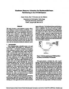
One of the major known facts about the human visual system is the existence of separate parallel processing pathways for form, color, and detail. Similarly, our system has parallel processing streams for features that come from a global form-based and gray-level statisticsbased analysis of each object, and for other features that measure local detail. Finally, our experience with hybrid neural network/knowledge base systems has convinced us that hybrid systems often succeed where the component systems fail. Consequently, our solution is a hybrid of the three major ATR processing methods: conventional image processing, neural networks, and knowledge based expert systems. 2.2. Pattern Processing Tasks In ATR An example of the sequence of tasks in an ATR system based on classical pattern recognition theory is shown in figure 2.2-1 (Bhanu, 1986). We will now examine these tasks, first the pattern processing tasks (section 2.2) and methods (section 2.3), and then the knowledge based reasoning tasks (section 2.4) and methods (section 2.5). Imaging Sensors object and background

-TV -LLTV -FLIR -SAR -MTI Radar -LADAR

Image Preprocessing -focus -image stabilization -noise suppression -contrast enhancement

Object Detection - object localization in imager FOV

Object Segmentation

Feature Extraction

-foreground/ background separation -silhouetting

-feature computation -feature parameterization -geometric -topological -spectral

Object Classification -linear classifiers -quadratic classifiers -cluster analysis -tree classifiers

object recognition indentification characterization

91iaf038

Figure 2.2-1: Conventional ATR System Architecture 2.2.1. Sensor Processing The digital data stream from the imaging sensor is the raw data input for all ATR systems. However, the bulk of the processing in an ATR system actually happens in the sensor itself. First, there is the optical processing by lenses on the incoming energy. Second, there is the recording of the spatial and temporal energy pattern. Third, those patterns are processed according to the sensor type (compared to the outgoing energy stream in SAR and LADAR, Doppler shift processed in MTI, etc.). Finally, the results are digitized. Clearly, in an ideal ATR solution, the specific sensor attributes must be taken into account implicitly via the choice of processing techniques or explicitly via a knowledge base. We have based our research on images produced with two different LADAR sensors; one produces range and intensity-of-return (reflectance) data; the other one produces range and passive infrared 17

R94061


(thermal) data. 2.2.2. Image Enhancement With image preprocessing, the image is enhanced in a way that helps separate object from background. In general, the image will have one or many objects in it, some of which are targets, while others are clutter that may look like potential targets. Also in the image is a background which surrounds the objects, and sensor noise superimposed on the whole image. The objective here is to provide low-level image processing (focus adjustment, image stabilization, and contrast enhancement) so as to enhance the target image relative to the background, without making the clutter look too target-like. 2.2.3. Object Detection The assumption is typically made that an image which has the same gray level for all pixels conveys no information. Any spatial variation in the gray levels is used as indication for the existence of “objects” in the image, where objects are considered representations for potential targets. An ideal object detection algorithm would provide coordinates for the locations in the image of each potential target. This evokes the question: how is “potential target” defined? In terms of LADAR, there are two data streams and hence two possible answers. In the range data, a potential target is anything that extends out of the terrain. In the intensity data, a potential target is any structure whose reflectivity for laser light is different from its surroundings. The fundamental difference between the two data streams results in different choices of processing methods. The intensity image is much more similar to the image perceived by the human visual system (as seen by one eye) than is the range image. The range image can be compared to the “disparity map” produced in higher vision by comparing the data streams from the two eyes. The fact that people with full vision in one eye, but none in the other, perform most visual tasks quite well confirms that the range data is not necessary for 3D perception. However, in an IU system where range data is readily available, such as in LADAR based ATR, it is probably the easiest source for 3D perception. The intensity data provides information about reflectivity and surface texture which is not available in the range data; we believe it can be included in the ATR process for improved performance. Chapter 7 describes the details of our research on how to include both the range and intensity data in detection and segmentation. 2.2.4. Object Segmentation If an ideal object detection algorithm provides the locations representing the centers of

18

R94061


objects, then an ideal object segmentation algorithm provides the outline of each object. Obviously, the center of an object cannot be calculated without some knowledge of the object’s extent; therefore the steps of detection and segmentation are inseparable. It is at this point that the conventional ATR process typically becomes more model-based and less signal-based. The models used for segmentation can be subtle and implicit, such as assuming connectivity of an object's edges, the existence of an inside and an outside of a 2D figure, etc. The models can also be quite explicit, such as maintaining a dictionary of target silhouettes which are optimally manipulated (i.e., scaled, translated, or rotated) and selected to provide the best match to the imaged object. This latter approach would be representative of the “model based vision” school of thought. Research in biological vision indicates that many functions of early vision, such as segmentation, do not depend on “top-down processing” and hence do not use explicit models which require references to a dictionary of any kind. Neuromorphic segmentation algorithms resulting from such research are discussed in section 3.1. Explicit models can still be extremely useful in ATR. We believe they are best used in segmentation for simple geometric object parts, such as ellipses (wheels) and long straight lines (cannon barrels, edges of buildings, etc.) rather than in segmenting whole objects. 2.2.5. Feature Extraction The next step after segmentation is to transform subimages, each containing one segmented image object, into a form which can be used as input by the neural classifier. This must be a 2-D to 1-D transform since classifiers work with vectors, not matrixes. Processing extracted features rather than direct image data also provides a form of data compression. In a high resolution image, each object might be represented by thousands of pixels, and if each pixel is considered a separate dimension in the classification problem, the performance of many classifiers becomes unacceptable. Additionally, most classifiers require all input patterns to be of the same dimensionality, but different objects generally have different numbers of pixels. In addition to these basic requirements, the transform should maximize the difference between objects of different classes while minimizing the difference between objects of the same class. This is highly domain dependent and generally much harder than the choice of a classifier. The underlying assumption is that if the features are statistically separable in the chosen feature space, then the associated objects will be separable in the object space; i.e., they will be classifiable. Therefore, the power of the features to provide adequate target distinguishability is critical, no matter what object classification scheme is chosen. Traditional feature extraction methods are discussed in section 2.3.2, and neuromorphic methods in section 3.2. 19

R94061


2.2.6. Classification Even if the feature space maximizes the similarity of objects in the same class and minimizes the similarity of objects in different classes, the general nature of ATR imagery makes feature based classification a very hard problem. A variety of classification schemes has been implemented and evaluated in past efforts, including classical linear and quadratic classifiers, statistical clustering, synthetic discriminant functions, and knowledge-based discriminators (see Bhanu, 1986 and Roth, 1990 for more complete listings). It is easy to prove that a simple Bayesian classifier is optimal, but the a priori probability distributions of all possible classes must be known. Those probabilities cannot be known in the ATR domain, and there is no basis for making simplifying assumptions such as Gaussian. This is why neural network classifiers have proven to be superior to statistical classifiers in a variety of applications; they need no a priori assumptions about the input data. Neural network classifiers are discussed in detail in section 3.3. 2.3. Pattern Processing Methods The following sections elaborate on the classical methods of image processing that are relevant to the IU tasks of image enhancement, object detection, and object segmentation (in section 2.3.1), and on traditional methods of feature extraction (in section 2.3.2). The neuromorphic approaches to both of these tasks are discussed in chapter 3. 2.3.1. Image Processing Image enhancement, object detection, and object segmentation are all 2-D to 2-D mappings, or image operations. The following is a taxonomy of the applicable processing methods. 2.3.1.1. Point Processes Any image processing which for each output pixel only takes into account the value of the input pixel at the same location (and possibly the coordinates of the location) is called a point process. The most common example is density slicing: each input pixel with value greater than a lower threshold and less than an upper threshold gets one value in the output image, while all input pixels with values outside of that range get another value in the output. Density slicing with just one threshold (one output value for input values below and another for values above the threshold) is simply known as thresholding. Density slicing in one form or another is a common method for object detection and segmentation4 and we use it in two different segmentation

4 It is an example of “region based segmentation”, which is based on the assumption that regions must be

20

R94061


methods, one using object height (see section 7.2.1) and another using the energy in object reflectance (see section 7.2.2). 2.3.1.2. Area Processes The definition of area processes is similar to that of point processes, but rather than using just one input pixel all input pixels within a given neighborhood are included in the computation of the output pixel which represents the center of the neighborhood. Most area processes are based on 2-D convolution and differ mainly in the choice of convolution kernel. The most common use for 2-D convolution in ATR is to detect and enhance edges as a part of the segmentation stage. Enhanced edges are used for “edge based segmentation”, where the assumption is that boundaries must be localized, based on the dissimilarity of nearby pixels, before regions can be distinguished. This assumption is also made in the neuromorphic segmentation methods discussed in section 3.1. 2.3.1.3. Frame Processes Frame processes use two or more whole images to produce one image. This has obvious application in motion detection and processing temporal image sequences in general, but we have also found use for frame processes in combining LADAR images from the range and intensity domains. 2.3.1.4. Histogram Operations From a histogram of the image gray-level pixel values, it is readily apparent whether the image is of high or low contrast. In particular, it becomes obvious if a range of values is unused or only used by a few pixels. It is then possible to generate a new distribution of values in order to use more of the neglected range. This operation does not change the information content of the image in any way, but it facilitates the gradient based separation of adjacent pixels which belong to different objects, and it makes the image easier for human observers to analyze. 2.3.1.5. Geometric Processes Scaling and rotation are geometric processes which are used in almost all image processing applications. In our system these transforms are used to normalize sub-images before they are classified.

distinguished, based on the similarity of nearby pixels, before boundaries can be localized. 21

R94061


2.3.2. Feature Extraction Candidate features (figure 2.3.2-1) range from simple geometric parameters, such as area, periphery, and orientation of best fitting ellipse, to more complex parameters representing the 2D or even 3D topology. Unfortunately, without model based vision, the extraction of topologically relevant features such as straight lines, closed boxes, ellipses, etc. is computationally expensive and error prone. Since targets exist in infinite variety, and model based vision is based on a finite (usually small) number of models, model based vision is of limited use in ATR. The gray level statistical characteristics of each object are easy to compute and parameterize. These features are based on all the pixels which lie within the boundary of each object, rather than just the boundary itself, as is the case with many of the geometric features. Typical statistical features are the mean, modal, and standard deviation density of the pixel gray level values for a given object. Gray Level Statistics

Model Based Attributes

Subobject Attributes

Geometric Attributes

Connectivity of Subobjects

Moments

Number of Subobjects Fractal Gabor Transform Signatures

Wavelet Mellin

Hilbert Fourier Based Object in Image

Fourier-Log-PolarFourier

Standard Deviation Gray Level Statistics

Cosine

Modal

Geometric Attributes

Mean

Aspect Ratio

Best Fitting Ellipse Attributes

Orientation Minor Axis Length

Periphery

Major Axis Length

Area Center-Of-Gravity Moments 2nd Moment Higher Moments

Figure 2.3.2-1: Object Feature Hierarchy

22

R94061


Other features which are also calculated over the entire object based on gray levels are transforms such as Gabor, wavelet, and fractal. These produce signatures which have been shown to contain most of the relevant pictorial information at a very significant data compression. Considerable research on compression methods has come from the study of visual image representation in the brain. The Gabor transform in particular has been used in a variety of ways to produce compact representations. It has the advantage of producing the minimal joint error in spatial frequency and location. The measures of spatial frequency and location obey an uncertainty principle which applies to all 2-dimensional transforms and the Gabor transform is the optimal solution with respect to information content (Gabor, 1946; Daugman, 1983; Daugman, 1988). 2.4. Knowledge Based Reasoning Tasks In ATR The following three sections (2.4.1 -2.4.3) define the three main ATR tasks that are not based on pattern processing and hence would not be executed on special neural/parallel hardware. 2.4.1. A Priori Knowledge Integration Exogenous information can be used to a great advantage, along with the primary data stream from the imaging sensor. First, the sensor viewing angles, such as field of view and horizontal and vertical angular resolution, are assumed to be known. If the sensor is mounted on an aircraft or a missile, the depression angle is typically also known. This information is useful for determining issues of perspective. Environmental information, such as the weather, time of day, and season can be used to influence the parameter settings of neural networks and decision rules with simple look-up tables. Similarly, mission information can be used to rule out certain target types, for example “tanks” when flying over oceans. Mission information can also be used to adjust the a priori probabilities of certain target types at a finer level of discrimination, for example to decrease the expectancy of finding one of your own tanks the further behind enemy lines you get. 2.4.2. Truth Data In order to train and verify the performance of a classifier, it is necessary to have truth data for all image objects used during training and verification: the class labels (“clutter”, “target”, “tank”, “bridge”, etc.) and the image coordinates of each object. The label can be considered a symbolic value and the coordinates the address for that value. For some testing purposes it is enough to manually compare the system’s output with the truth data, but this is error prone and becomes unfeasible for large scale testing. Training would 23

R94061


also quickly become intractable if the correct class for each object had to be looked up manually. Consequently, truth data must be available on-line and in a format that allows the ATR algorithm to automatically find the class label for a given object. The ATR algorithm must be able to compute image coordinates (address) for each segmented object and use them to look up the label (symbolic value). The problem is that this addressing system is continuous valued and therefore the probability of the ATR-generated address matching one of the addresses in the truth data is infinitesimally small. Some processing is required to find the “closest” (according to some metric) address in the truth data and then to determine if that is “close enough” to be considered the address of the same object. Only then can the symbolic value be determined. 2.4.3. Decision Fusion Any system which contains multiple parallel channels, where the same data is analyzed independently in each channel (see chapter 7), must confront the issue of how to combine the different analyses into one coherent decision. This can be done with simple logic, such as requiring agreement between certain channels for a given category to be selected. A more flexible approach is to use either fuzzy logic or confidence voting, where the decision from one channel is used to qualify the decision from another. 2.5. Knowledge Based Reasoning Methods The standard method for performing knowledge based reasoning is with expert systems. The following four sections provide an overview of expert systems and their applicability to ATR. 2.5.1. Expert System Overview An expert system is a computer program that can perform a task that normally requires the reasoning ability of a human expert. Expert systems are highly specialized according to their application domains. Although any program solving a particular problem may be considered to exhibit expert behavior, expert systems are differentiated from other programs according to the manner in which the domain specific knowledge is structured, represented, and processed to produce solutions. In particular, expert system programs partition their knowledge into the following three blocks: Data Base, Rule Base, and Inference Engine. Expert systems utilize symbolic and numeric reasoning in applying the rules in the Rule Base to the facts in the Data Base to reach conclusions according to the construct of reasoning specified by the Inference Engine. There are two basic types of knowledge that can be incorporated into expert systems: declarative knowledge and procedural knowledge. The kind of knowledge describing the

24

R94061


relationships among objects is called declarative knowledge. The kind of knowledge prescribing the sequences of actions that can be applied to this declarative knowledge is called procedural knowledge. In expert systems, procedural knowledge is represented by production rules whereas declarative knowledge is represented by frames and semantic networks, in addition to production rules. While expert systems have been traditionally built using collections of rules based on empirical associations, interest has grown recently in knowledge-based expert systems which perform reasoning from representations of structure and function knowledge. For instance, an expert system for digital electronic systems troubleshooting is developed by using a structural and behavioral description of digital circuits (Davis, 1984). The objective of this approach to expert system implementation is to reason from first principles about the domain rather than from empirical associations. One of the key ideas in this approach is to use multiple representations of the digital circuit (both functional and physical structure) in troubleshooting applications. The approach is also similar to the multiple levels of abstraction in modeling of mental strategies for fault diagnosis problems (Rasmussen, 1985). 2.5.2. Qualitative Process Theory Qualitative Process (QP) theory (Forbus, 1988) is another approach allowing the representation of causal behavior based on a qualitative representation of numerical knowledge using predicate calculus. QP theory is a first order predicate calculus defined on objects parameterized by a quality consisting of two parts: an amount and a derivative, each represented by a sign and magnitude. In Qualitative Process theory, physical systems are described in terms of a collection of objects, their properties, and the relationships among them within the framework of a first order predicate calculus. Hierarchical knowledge representation at several levels of abstraction is also another approach used in modeling human problem-solving strategies for complex systems (Rasmussen, 1985). This hierarchy is two dimensional. The first dimension is the functional layers of abstraction for the physical system: functional purpose, abstract function, generalized function, physical function, and physical form. The second is the structural layers of abstraction for the physical system: system, subsystem, module, submodule, component. 2.5.3. Inference and Reasoning Strategies The inference control strategy is the process of directing the symbolic search associated with the underlying type of knowledge represented in an expert system: antecedents of IF-THEN rules, nodes of a semantic net, or collection of frames. In practical expert system applications, the

25

R94061


blind search is an unacceptable approach due to the associated combinatorial explosion. Search techniques can be basically grouped into three: breadth-first, depth-first and heuristic. The breadth-first search exhausts all nodes at a given level before going to the next level. In contrast, the depth-first exhausts all nodes in a given branch before backtracking to another branch at a given level. Heuristic search incorporates general and domain-specific rules of thumb to constrain a search. Expert systems employ basically two types of reasoning strategies based on the search techniques above: forward chaining and backward chaining. In forward chaining, starting from what is initially known, a chain of inferences is made until a solution is reached or determined to be unattainable. For instance, in rule based systems, the inference engine matches the left-hand side of rules against the known facts, and executes the right-hand side of the rule that is activated. In contrast, backward-chaining systems start with a goal and search for evidence to support that goal. Pure forward chaining is appropriate when there are multiple goal states and a single initial state whereas backward chaining is more appropriate when there is a single goal state and multiple initial facts. Many expert systems utilize both forward and backward chaining. 2.5.4. Knowledge Bases for ATR In hybrid ATR, knowledge base processing can be employed in a variety of ways. An executive knowledge base can control the operation of the entire hybrid system. Knowledge bases can be developed for target classification and decision fusion. Neural network learning can be controlled by a knowledge base. In addition, the symbolic processing power of knowledge based expert systems are ideal in interpreting the numeric outputs of neural networks. Other KBs can be implemented to encode subsystem capabilities/constraints and lower-level target classification and identification functions.

26

R94061


3. Neural Paradigms for IU As discussed in section 1 of this report, the main IU tasks that could be solved using neural network methods are: • Image segmentation • Feature extraction • Classification Sections 3.1 - 3.3 discuss in more detail the neural networks and other neuromorphic approaches that are appropriate for each of these tasks. One other neuromorphic design option that does not fit under any of those three tasks is also discussed here (in section 3.4): sensor design based on foveal vision. 3.1. Image Segmentation The most promising neural network paradigms for image segmentation that we have identified in this research effort are the Boundary-Contour-System/Feature-Contour-System (BCS/FCS) (Grossberg & Mingolla, 1985; Grossberg & Mingolla, 1987) and its derivative systems. The effectiveness of the BCS/FCS in preprocessing synthetic aperture radar images has been demonstrated by Grossberg, Mingolla & Williamson, 1993 and Cruthirds et al., 1992, and independently by Waxman, Seibert, Bernadon & Fay, 1993. The BCS detects edges and completes sharp boundaries over gaps in image contours. The FCS fills in areas segmented by the BCS with gray levels that represent surface properties of reflectance and texture, discounting effects of uneven illumination. The remaining segmentation task of isolating individual objects becomes much easier because object boundaries are continuous. Carpenter, Grossberg & Mehanian, 1989; Grossberg & Wyse, 1991; and Bradski & Grossberg, 1994 have demonstrated a complete segmentation system called CORT-X 2 which is based on BCS/FCS using simulated LADAR data. Other segmentation systems exist that are also promising but not as well tested as the BCS/FCS systems; there is one, for example, by Heitger & Heydt, 1993 and one by Finkel & Sajda, 1992. The common factor in all these systems is that they attempt to model the primate visual system’s approach to detecting and completing closed contours in images of 3-D scenes. They are not developed specifically to solve problems in computer vision, and hence they are not designed with regard for computational efficiency on conventional computers. Consequently, even though these systems are considered promising by many researchers in IU, they are also criticized for being too slow for many applications (for example all real-time applications). The

27

R94061


benefit from a neural hardware implementation that provides a major improvement in computational efficiency for these systems is therefore of great significance. Output Cooperative Layer

2nd Competitive

Filling-In

1st Competitive FCS System

Oriented Filters

BCS System

Contrast Enhanced

Image

Figure 3.1-1: The BCS/FCS System Figure 3.1-1 shows a block diagram of the complete BCS/FCS system. The system was developed as a model of low-level human vision that can account for a variety of perceptual phenomena, such as boundary completion, brightness perception, binocular rivalry, and motion detection. Consequently, there is significant leeway for simplification when the purpose is “just” to do segmentation. The most obvious simplification is to eliminate the FCS, since its primary purpose is to model brightness perception. Following the layout shown in figure 3.1-1, the image first gets contrast enhanced by a preprocessing layer that models the retina. The nodes in that layer are laterally cross-connected to allow short-range center-surround competition. This is similar in effect to convolving with a 2-D circularly symmetric (isotropic) Mexican-hat shaped function. 28

R94061


The first layer in the BCS contains oriented filters that model the simple and complex cells in area V1 of visual cortex. The simple cells are modeled as elongated contrast detectors that determine the approximate position and orientation of image contrast. By adding the outputs from pairs of simple cells it is possible to model complex cells: if the simple cells are tuned for identical position and orientation but opposite direction of contrast (for example left-to-right and right-to-left in a vertically oriented pair), then the combined output is insensitive to direction of contrast. This is a form of edge detection. Since each oriented filter is only sensitive to one orientation at one location, multiple layers of these filters are needed. The nodes in one layer all code the same orientation and the 2-D location is coded topographically. The positional resolution is therefore determined by the number of nodes in a layer (typically one per pixel) and the orientational resolution is determined by the number of layers (typically 8 or 12). This organization holds for every stage in the BCS. The basic operation of the 1st competitive stage is to provide inhibition of spatially neighboring nodes with the same orientation. This is similar to convolving with a 2-D isotropic Mexican-hat function within each orientation layer. The 2nd competitive stage performs a competition across orientation layers such that inhibition is greatest between cells with perpendicular orientations at the same location. This is a push-pull opponent process, such that when one orientation is excited the perpendicular orientation is inhibited and when one orientation is inhibited the perpendicular orientation is excited by disinhibition. The combined functions of the 1st and 2nd competitive stages are: (1) to sharpen any orientation signals (edge elements) present in the system, and (2) to produce so called “end-cuts” at the ends of thin lines. End-cuts look like small line segments at the line ends, similar to the short horizontal segments at the top and bottom of an “I”. They code the location and orientation of line ends for further processing, enabling both completion of boundaries across gaps between collinear line ends and the formation of illusory contours (figure 3.1-2).

29

R94061


Figure 3.1-2: Horizontal Boundary With Gaps (top) and Horizontal Illusory Contour (bottom) The cooperative layer performs a long range cooperative process for boundary completion. The cells in this layer are called bipole cells because they have oriented receptive fields in two lobes. For example, a vertically oriented cell’s receptive field looks like a vertically stretched “8”. A bipole cell that gets sufficient input to both lobes feeds an output signal back to the 1st competitive stage at a location midway between the two line elements that contributed the inputs to the two lobes. If these line elements were line ends then the feedback synthesizes a new line element in the middle of the gap between the line ends, creating two smaller gaps. On the next round of the feedback loop, other bipole cells will put new line elements in the middle of each of those gaps, and so on until the line elements form a continuous boundary. Due to the end-cuts, bipole cells can also form continuous boundaries across line ends that are not collinear, such as in the illusory contour that we see between the misaligned line ends in the lower half of figure 3.1-2. This ability is known to be essential to primate vision (von der Heydt & Peterhans, 1989), but it is still ignored in most machine vision systems. The segmentation is complete when the feedback loop has reached equilibration. In typical implementations it has proven sufficient to loop a few times (5 at most), rather than explicitly testing for some criteria of equilibration. Since the FCS is not required for segmentation, it will not be detailed here; the reader is referred to one of the original references, such as (Grossberg & Mingolla, 1987). 3.2. Feature Extraction There are two basic approaches to extracting features: a global feature is one scalar value based on the whole subimage, while local receptive field features for one subimage are computed

30

R94061


by applying a 2-D function to regularly spaced locations in the subimage, similar to processing of the retinal image at various levels of the visual pathway in mammals. Gabor functions are an elementary type of function which have been very useful in a variety of image processing and analysis applications. Essentially, a Gabor function is the product of a Gaussian and a complex sinusoid. These functions were discovered in 1946 by Denis Gabor in connection with information theory. While their origin is non-neural, they are often considered neuromorphic functions due to their excellent fit with measured responses from living neurons. Daugman, 1980 was first to generalize Gabor functions to two dimensions and use them for modeling the properties of receptive fields of simple cells in the visual cortex of cats. Part of the appeal of using Gabor functions for machine vision is that they have been so useful in describing neurons in visual cortex; this suggests that there is a substantial benefit to using these functions for vision. This development in many ways parallels the discovery of so-called edge-detectors by Hubel & Wiesel in the 1960's and the subsequent proliferation of edge-detecting algorithms in computer vision. Interestingly, Gabor functions with parameters tuned to match simple cells in the visual cortex can be thought of as detecting lines and edges as well. Examples of the Gabor functions used are shown in figure 3.2-1. The real part of the Gabor function (cosine) is shown on the left, and the imaginary part (sine) is shown on the right. It is not difficult to see how the kernels on the left can be viewed as line detectors and the kernels on the right as edge detectors.

Figure 3.2-1: Gabor Functions in 12 Different Orientations

31

R94061


The main properties of Gabor functions are that they are localized in both space and spatial frequency. This means that when a particular Gabor function is multiplied by a 2-D signal (image), the resulting coefficient represents a sensitivity to a specific frequency at a specific location in the image. Gabor functions also minimize the joint uncertainty of the two domains (Daugman, 1985). This is really just another way of saying that Gabor functions localize a signal in both space and spatial frequency (or time and frequency) in an optimal way. This property suggests that using Gabor functions in coding applications would result in an optimal strategy. A 2-D Gabor function, or filter, can be tuned to a specific frequency (cycles/image) and orientation (degrees or radians measured from one axis). 2-D Gabor filters optimally and uniquely achieve simultaneous localization in space and in spatial frequency. A properly tuned filter can be used as a correlation filter to look for energy in an image at a particular frequency and orientation. Used in this manner, these filters can produce features that represent object texture. Any real-valued image can be expressed as a weighted sum of appropriately shifted Gabor functions. The set of complex-valued weighting coefficients represent the Gabor transform of the image. These coefficients yield localized spectral information about the image, as the coefficients having relatively large magnitudes for a given spatial location correspond to the dominant frequencies occurring in that spatial vicinity. In fact, the original subimage can be reconstructed exactly from these coefficients. Since feature extraction should compress the information available in the subimage, we use a sparse sampling of the image when applying the Gabor filter. (No compression would imply performing a complete convolution, where the filter is applied separately to every pixel). Objects also have to be scaled such that they all have the same dimensions. This is necessary because of the sparse sampling: the number of locations must be fixed (since the feature vector length must be fixed) and we also want to sample all objects with the same resolution. The only way to accomplish both is to scale each object such that it fits in a subimage of fixed dimensions.

32

R94061


Figure 3.2-2: Sampling Grid for Local Features We used a sampling of 9 locations (3x3 grid) on square subimages of dimensions 64x64 pixels, as shown in figure 3.2-2. Each circle indicates 12 oriented Gabor features5 with orientations laid out as the hour marks on a clock (one every 15°). Each of the 12 filter pairs shown in figure 3.2-1 is applied, generating sine and cosine coefficients representing 12 evenly spaced orientations for each sampling point. To compress even further, the sine and cosine coefficient pair is converted to a magnitude and phase coefficient pair and the phase value discarded. This is a safe assumption because the phase codes local position within the 32x32 box, which is not very meaningful for texture extraction. Consequently, we get 12 coefficients per sampling point; for 9 points that produces 108 coefficients which we use as a feature set representing one subimage. 3.3. Classification Neural network classifiers have proven to be very useful in the ATR work of a number of researchers (see Roth, 1990 for a review). Our own research (Caglayan et al., 1992; Snorrason et al., 1993) has indicated that neural network classifiers may be ideal for ATR, in terms of both accuracy and robustness. In particular, our ATR research has shown that adaptive resonance theory (ART) neural networks perform very well as target classifiers when presented with features extracted from segmented image objects. In the next two subsections (3.3.1 and 3.3.2) we will analyze in more detail two important

5 Each Gabor function was implemented with a 32x32 pixel kernel, frequency 2.5, aspect ratio 0.5, and standard

deviation 0.25, as shown in figure 3.3-1. 33

R94061


issues of classification, invariance and feature selection, and explain how they can be dealt with using neural networks. Following that (3.3.3), we will explain our choice of paradigm for a neural network classifier, the Fuzzy-ARTMAP, and give an overview of its operation. 3.3.1. Invariance Invariance towards scaling, rotation, and distortion due to perspective change is possibly the hardest unsolved problem in object classification. Common neural network approaches to invariance can be divided into the following three groups (Barnard & Casasent, 1991) First, the structure of the neural net can be designed to make the net capable of invariantly classifying input objects. Second, the network can be directly trained to recognize the same object under different transforms. Third, a set of invariant neural network input features can be created from the input objects. 3.3.1.1. Structural Invariance The best known example of this approach is the Neocognitron neural network which has been shown to recognize handwritten letters invariantly with respect to translation, scale, and certain other deformations (Fukushima, Miyake & Ito, 1983; Fukushima, 1989). The approach is biologically inspired: the Neocognitron has multiple layers where the higher layers encode local combinations of features in lower layers. However, this invariance is achieved at a very high cost in brute force redundancy and extensive hand tuning of connectivity and parameters (Menon & Heinemann, 1988;Barnard & Casasent, 1991). It is therefore unlikely that this approach can be scaled up to the complexity of ATR. However, structural invariance can be used to look for specific features (such as wheels) on an object which has already been determined to be of a particular target type (such as a tank). 3.3.1.2. Training Based Invariance This approach is based on the basic ability of all neural networks to generalize: simply show the network enough examples of the same object at different orientations, scale, etc. until it has learned to recognize the object invariantly. The problem is that this training may have to be done for every object which the network is intended to recognize. In ATR, where the number of targets to be recognized is potentially very large, this approach is clearly not sufficient but it can still be used to recognize specific object features, in a similar way as the structural invariance method. 3.3.1.3. Invariant Feature Extraction It is often possible to compute features which are invariant to a set of transforms. For example, the Fourier-Log-Polar-Fourier transform has been shown to be invariant to translation, 34

R94061


rotation, and scale (Cavanagh, 1984). This is unfortunately at the cost of losing all the phase information from the Fourier transform, which affects discrimination. It has still been used with considerable success to categorize simple silhouette images (Carpenter et al., 1989). Given the multiple other reasons for computing features (improved discrimination, data compression, etc.), it seems logical to use invariant features to solve the invariance problem. It does not change the overall system design, but merely affects the choice of features to compute. This is the approach we have taken, along with the use of projection to a “virtual” top view in the LADAR data (explained in section 7.1), to get invariance to translation, rotation in 3-D, and range. 3.3.2. Feature Selection In our sample ATR results (section 7.4.1) we generated a set of 56 features from each of the image objects produced by the segmentation module. This large number of features is typical of IU applications. Unfortunately, “the curse of dimensionality” applies here. It is a well known problem for all pattern recognition methods (neural or otherwise) which basically states that the higher the number of dimensions in the input space, the more training patterns are needed to properly sample the space. As a rule of thumb, the minimum number of training patterns should be 5-10 times as many as the number of dimensions. Since most IU development is done with a limited set of images, there is a limit to the number of features that can be added before recognition accuracy starts going down due to the curse of dimensionality. Also, some features are computationally expensive (such as fractal measures) and can only be included in a real-time IU system at the expense of other features, given that there is a fixed amount of time allocated for computing all features. In summary, more is not always better when it comes to selecting features. We have formulated a solution based on an extension to our simplified Fuzzy-ARTMAP neural classifier that learns the relative importance of different features for a given set of training patterns. By choosing only the most important features, it is no longer necessary to compute every extracted feature for each input vector. This novel solution can potentially benefit all highspeed uses of Fuzzy-ARTMAP since it guaranties that only the minimum number of features is computed for each input vector. This work, which is still in development, was inspired by work by Aguilar & Ross, 1994. This research does not directly affect the choice of hardware: it is an extension to Fuzzy-ARTMAP and we expect all the same hardware that is well suited for FuzzyARTMAP to be also appropriate for this system. There is another side to feature selection: in simpler classification problems it is easier to use intuition to select features with good discriminant qualities. Consequently, we have divided the ATR problem into separate classification problems, which are hierarchically related. Each level

35

R94061


in the hierarchy represents a level of discrimination. The first (coarsest) level only discriminates between “targets” and “clutter”. The next level only looks at “targets” and discriminates between major classes of targets, such as “buildings”, “bridges”, and “vehicles”. The finest level discriminates between target types in each class, such as between “tanks” and “other vehicles” in the class “vehicles”. By identifying which features are most discriminant for each classifier (such as high fractal dimension for natural “clutter” objects and low for man-made “target” objects), it is possible to select just a few key input features for each classifier, hence the reduction in dimensionality. 3.3.3. Fuzzy-ARTMAP When the issue of classification using neural networks is brought up, the Back Propagation (BP) neural network paradigm is often suggested. We have used BP neural networks with some success on pattern recognition problems, but we have found supervised learning Adaptive Resonance Theory, or ARTMAP (Carpenter, Grossberg & Rosen, 1991), neural networks significantly more powerful. Some of the features that distinguish ARTMAP networks from other neural networks, such as BP, Kohonen, Radial Basis Function (RBF), and Hopfield networks: •

Self-organizing architecture: No network architecture needs to be specified. Weights are added as needed during training to guaranty that predictive error is minimized while generalization is maximized.

•

Fast learning: ARTMAP networks are capable of learning input-output patterns given a single presentation. This should be contrasted against the thousands of epochs needed to train BP, RBF, and Hopfield nets.

•

Stable learning: ARTMAP networks always achieve correct and stable classification of the training set. This can be contrasted with local minima and forgetting in the other networks. For example, using the ARPA benchmark of “circle-in-square”, ARTMAP will get 100% performance on the training set within 5 epochs, while BP's best performance is 80%-90% and is achieved after a few thousand epochs.

•

Online learning: ARTMAP networks can be taught on-line in “real-time”. There is no need to distinguish between a training phase and a test phase, allowing the system to adapt continuously in a continuously changing environment. Conversely, if after a certain amount of training no further adaptation is desired then training can be turned off.

36

R94061


•

Incremental learning: After having learned to classify a set of inputs, ART systems are capable of learning to classify additional types of information without having to be completely trained. This feature allows the addition of new uncalibrated sensors to a previously trained system without having to retrain the system.

•

Immediate access to categories: After learning a category, ARTMAP networks can choose that category in a single pass through the network without any iterative computations. This feature allows for very fast performance during deployment of the system.

•

Confidence Level: ART systems also provide a measure of confidence in their predictions. This confidence level is a computation of the degree of membership of the input vector in the category's template. This confidence measure can be used to bias the global decision making process. None of the other neural networks provide a confidence value.

•

Control via a single parameter: ART system performance can be controlled using a single parameter, called vigilance. Low vigilance produces coarse categorization, while higher vigilance produces finer categorization. In contrast, BP requires several parameters such as momentum and learning rate. Furthermore, the effect of varying these parameters on the final system classification is not clear. 3.3.3.1. The Original Version

Fuzzy-ARTMAP (Carpenter et al., 1991) is a supervised neural network classifier that learns to classify inputs by a fuzzy set of features, or a pattern of fuzzy membership values between 0 and 1 indicating the extent to which each feature is present. This way the ARTMAP’s disadvantage of only processing binary patterns is removed without affecting the various advantages listed above. Fuzzy-ARTMAP also differs from most other fuzzy pattern recognition algorithms in that it learns each input as it is received on-line, rather than by performing an offline optimization of a criterion function.

37

R94061


Figure 3.3.3.1-1: Fuzzy-ARTMAP Block Diagram A fuzzy ARTMAP system, as shown in figure 3.3.3.1-1(Carpenter et al., 1991), consists of a pair of fuzzy ART classifiers (ARTa and ARTb) that create stable recognition categories in response to arbitrary sequences of input patterns. During supervised learning, ART a receives a stream a(p) of input patterns, and ARTb receives a stream b(p) of input patterns, where b(p) is the correct prediction given a(p). These modules are linked by an associative learning network and an internal controller that ensures autonomous system operation in real time. The controller is designed to create the minimal number of ART a recognition categories, or “hidden units”, needed to meet accuracy criteria. It does this by realizing a “minimax” learning rule that enables the fuzzy ARTMAP system to learn quickly, efficiently, and accurately as it conjointly minimizes predictive error and maximizes predictive generalization. This scheme automatically links predictive success to category size on a trial-by-trial basis using only local operations. It works by increasing the vigilance parameter ρ a of ARTa by the minimal amount needed to correct a predictive error at ARTb. When the ARTa classifier is presented with an input vector a, the bottom-up activation from a F1 causes the F2a layer to choose a category node based on the input’s fuzzy membership in that Fa category's fuzzy set. The chosen category then sends information back to the 38

1

layer which is

R94061


compared to the input vector a. The fuzzy intersection of top-down activation with the input vector produces a match value that indicates the classifier's confidence in its category choice. Parameter ρ a calibrates the minimum confidence that ARTa must have in a recognition category, or hypothesis, activated by an input a p in order for ARTa to accept that category, rather than search for a better one through an automatically controlled process of hypothesis testing. Lower values of ρ a enable larger categories to form, leading to broader generalization and higher code compression. A predictive failure at ART b increases ρ a by the minimum amount needed to trigger hypothesis testing at ART a , using a mechanism called match tracking (Carpenter, Grossberg, and Reynolds, 1991). Match tracking sacrifices the minimum amount of generalization necessary to correct a predictive error. Hypothesis testing leads to the selection of a new ARTa category, which focuses attention on a new cluster of ap input features that is better able to predict b(p). 3.3.3.2. Our Simplified Version The full implementation as described in the previous section is rarely needed, as it is intended to associate an arbitrary output pattern with each input pattern. This association is a mapping between clusters of input patterns and clusters of output patterns, and these clusters can be formed with a controlled degree of “looseness” or variance, adjustable via the base-vigilance of the Fuzzy-ART clustering mechanism. Since there is one Fuzzy-ART for the inputs and one for the outputs, there are two such parameters. The base-vigilance for the inputs is generally set low, often at the minimum (0.0) in order to form the largest clusters possible. This is desirable because larger clusters usually provide better generalization.

39

R94061


Output Class

F3: Class layer

O1 O 2

OM

F2: Cluster layer

C1 C2

CK

Weights

Reset

ρ

Vigilance

W 21

F1: Input layer (a, ac )

Input (a)

Match tracking

I1

I2

I2N

Input Pattern Figure 3.3.3.2-1: Simplified Fuzzy-ARTMAP Architecture

The base-vigilance for output clustering is typically set very high, often at the maximum value (1.0) in order to be able to predict outputs precisely. When the base-vigilance of the output clustering mechanism is at the maximum value, it is possible to use a direct mapping from each input cluster to a set of output values instead of the more complicated output clustering (the ARTb module in figure 3.3.3.1-1) and a map. It is also the case that an output can normally be designated with one number, often an integer. The system implemented here is a complete Fuzzy-ART input clustering mechanism (F1 and F2 layers in figure 3.3.3.2-1) with a mapping for each cluster to a non-negative floating-point value (F3 layer). This simplified Fuzzy-ARTMAP system is coded in C++ as an independent class. There is a public interface consisting of 10 functions and some error constants. All data structures and internal functions are hidden from the user of the class. We have integrated the code into Khoros by writing the necessary interface functions; it can therefore be used just as any other built-in Khoros function in the Cantata visual programming language. This implementation has been tested on several data sets against the version of ARTMAP which was used in the original Fuzzy-ARTMAP papers and shown to produce identical results.

40

R94061


3.4. Uniform vs. Space Variant Resolution Sensors The problem with sensors which have a uniform resolution across the entire field of view is that an increase in resolution by n pixels in each direction leads to an n2 increase in the data produced. This causes all further processing on whole images (such as segmentation) to slow down. High resolution, however, is only needed on the objects, not on the background. Therefore, it is important to partition the image into small sub-images, each containing one object, as early in the processing chain as possible. This reduces the impact of the large amounts of data for the classification problem but not for the segmentation problem. Another problem which is specific to scanning sensors such as LADAR is that the time taken to scan in each image also increases by n2 . This can be a serious problem if either the sensor or the target is moving rapidly since the image will be distorted. The solution used in the visual system of all higher mammals is to use space variant resolution. A high resolution “fovea” consists of a small area in the middle of the field of view surrounded by a low resolution “periphery”. This leads to a data compression of 1:10,000 in humans (Rojer & Schwartz, 1990). The drawback is that some additional mechanism is required to rapidly move the sensor so each object can be re-analyzed foveally once it has been segmented. Once again, a biomorphic solution is available: the ocular motor system evolved as a solution to the same problem in mammals. This approach has been used in machine vision (Weiman, 1988 ;Weiman, 1989; Yeshurun & Schwartz, 1989; Sandini, Bosero, Bottino & Ceccherini, 1989; Abbot, 1991) and shown to have the additional advantage of leading to a much smaller and cheaper sensor (van der Spiegel et al., 1989; Bederson, Wallace & Schwartz, 1992). We have not opted for this solution in our proposed ATR system because we felt that too much custom hardware was required; it would take a disproportionate part of our development resources and it could compromise prospects of commercialization. We are well aware, however, of the importance of this research topic and we are prepared to re-evaluate our position if need be in Phase II. In particular, we have developed ties with Eric Schwartz’s lab at Boston University, where ARPA sponsored work on foveal vision has been producing very promising results (Bederson et al., 1992).

41

R94061


4. Hardware Options for Neural Networks The overwhelming majority of IU research with neural networks has been done with conventional digital computers: workstations and PCs. Many researchers have said that this system design is inappropriate because conventional digital computers are serial and neural networks are inherently parallel. One of our main research objectives was to assess the validity of this statement with respect to the IU domain. We investigated the currently available hardware options that in one way or another can be used to accelerate neural networks. In this chapter, we construct a taxonomy of computational hardware applicable to neural networks and IU. For each class of hardware in our taxonomy, we have tried to answer these questions: • • •

Relative to general purpose computers, how much of a speed improvement can this hardware offer? How scaleable are designs implemented on this hardware? What is involved for the software developer to transition an existing design from a general purpose computer to this hardware?

4.1. Types of Parallelism The architectures of parallel systems—how the processors connect to each other and to memory, and how the memory is configured (shared or distributed)—vary widely. How these architectures communicate with storage systems such as disks or mass storage and how they network with other systems also differ. The systems are distinguished by the kind of interconnection between processors (known as processing elements or PEs) and between processors and memory. Flynn’s taxonomy (Flynn, 1966) classifies parallel computers according to whether all processors execute the same instructions at the same time (single instruction/multiple data, SIMD) or each processor executes different instructions (multiple instruction/multiple data, MIMD). Conventional serial computers are also included in Flynn’s taxonomy: single instruction/single data, SISD. However, pipelined processors in modern serial computers can be thought of as using some parallelism, possibly best described as multiple instruction/single data, MISD. Many software systems have been designed for programming parallel computers, both at the operating system and programming language level. These systems must provide mechanisms for partitioning the overall problem into separate tasks and allocating tasks to processors. Such mechanisms may provide either implicit parallelism, where the system (the compiler or some other program) partitions the problem and allocates tasks to processors automatically, or explicit

42

R94061


parallelism where the programmer must annotate his program to show how it is to be partitioned. It is also usual to provide synchronization primitives such as semaphores and monitors to allow processes to share resources without conflict. Processors communicate via some kind of network or bus or a combination of both. Memory may be either shared memory (all processors have equal access to all memory) or private (each processor has its own memory, distributed memory) or a combination of both. Communication between tasks may be either via shared memory, in a multiprocessor, or message passing, in a multicomputer. Either may be implemented in terms of the other and in fact, at the lowest level, shared memory uses message passing since the address and data signals which flow between processor and memory may be considered as messages. The processors may either communicate to solve problems cooperatively, or they may run completely independently, possibly under the control of another processor which distributes work to the others and collects results from them, a processor farm.

System Type SISD

Architecture Type Pipelined Processor

Vector Processor

SIMD

Software Type

Algorithmic Parallelism

Systolic Array

Parallel Processor

Data Parallelism

Multiprocessor

Shared Variable

Multicomputer

Message Passing

MIMD

Figure 4.1-1: Types of Parallelism 43

R94061


Figure 4.1-1 summarizes the relationship between Flynn’s taxonomy, actual hardware architectures and the software paradigms they support. 4.2. General Purpose Computers 4.2.1. Single CPU Processing While the focus of this research is not on general purpose computers, it is important to be aware of the “baseline” options since almost all neural networks are developed on general purpose computers before being ported to special purpose or custom hardware. Developing IU software for uniprocessing systems simplifies the translation from first prototype to final product, relative to developing for multiprocessor systems. Often the workstations or PCs used during development use the same CPUs as the final system, such as Intel 80x86 or Pentium, Motorola 680x0 or PowerPC, DEC ALPHA, and SUN SPARC. These processors support a large variety of development tools, and by allowing engineers to work in familiar environments they can greatly speed up the development cycle. By limiting the design to uniprocessor capabilities, however, the IU tasks that can be performed in real time and/or on large images also become limited. A system designer faced with insufficient CPU throughput typically has two main options: replace the CPU with a higher performance processor or switch to a parallel processing solution. As discussed before, neural IU systems may benefit relatively more from parallel implementations than from increased performance uniprocessors. Therefore, designing for future scalability suggests looking for parallel solutions. 4.2.2. Distributed Processing The only way to take advantage of the inherent parallelism of IU systems, while using conventional SISD workstations and PCs, is to distribute processing over a computer network. Since the typical research lab has a local area network (LAN), it is possible to run software that distributes itself over the LAN so that the different tasks run on different computers at the same time. The main advantage to this approach is that it allows research on coarse-grain, parallel neural-network implementations, without investment in true parallel hardware. A few software development systems are available that make this possible even for developers that have no background in networking: Khoros (described in section 6.1) for a network of Unix computers and Power Tap6 for a network of Macintosh computers. This solution is unfortunately not

6Made by Always Thinking, Inc., Glen Allen, VA. Information available at [email protected] 44

R94061


applicable in many IU applications because it relies on the existence of a network of host computers. That rules out most applications which must run in the field in self-contained hardware, such as object detection from a moving vehicle. 4.3. Accelerators and Parallel Computers This section discusses the use of commercial hardware that is intended to speed up any compute intensive task; i.e., the hardware is not specialized for neural networks. 4.3.1. High Speed Co-processors A single, high-speed floating point co-processor (FPU) that plugs into the host workstation or PC’s motherboard is the simplest and least expensive way to speed up any algorithm that uses extensive floating point arithmetic, such as typical neural network algorithms. Porting a neural network developed on the host is very simple since no algorithmic changes are needed; only a recompilation of the source code is required to generate the proper machine code for the floating point operations. Although this approach has been very popular in the past, it is rapidly becoming obsolete because most modern CPUs now come with high-speed FPUs on-chip. For example, the FPUs in Motorola’s PowerPC CPU and DEC’s Alpha CPU are significantly faster than most stand-alone FPU chips. In other words, if a CPU such as the PowerPC or Alpha is not fast enough for a given IU application then recompiling for a another co-processor is not going help. We do not consider this solution powerful enough for most IU applications. 4.3.2. High Speed Accelerators A single CPU computer on a plug-in card goes by different names depending on the intended market; we will use the generic term accelerator here to emphasize the general purpose nature of this solution compared to the special purpose neural hardware discussed later. An accelerator provides more speed and flexibility than a co-processor because it has most of the functions of a full-fledged CPU. Typical accelerator processors are DSP (such as Analog Devices SHARC) or RISC processors (such as Intel i860). The accelerator is still dependent on the main CPU (the host) for outside world interfacing (to the user or to other systems), but once the data has been loaded, it can process one algorithmic task while the host performs another. It is possible to treat the accelerator just like a co-processor and have the host wait while the accelerator performs the floating point operations, but if there are two processing tasks in the algorithm which can run independently then the host and accelerator can perform them concurrently. The cost of this flexibility is that the source code must partitioned. The application tasks are 45

R94061


usually not distributed evenly between the main CPU and accelerator. The main CPU still has to take care of all data I/O to the external world (or to disk) and then make the data available to the accelerator via some shared memory setup. Hence, the routines that handle user interface and data I/O to the external world have to be manually separated from the main algorithm since these are typically not supported by the accelerator. For each concurrent pair of tasks the code must also be split up and compiled separately. Even if the performance increase relative to running without an accelerator can be significant, there is still the issue of scalability. An accelerator’s maximum speed is mainly a function of the architecture of the accelerator’s processor and its clock speed, both of which are usually set by the manufacturer. If the application’s performance requirements increase much beyond the originally expected requirements then the accelerator may no longer be a feasible solution. 4.3.3. Coarse Grain Parallel Computers The next step up in performance and price is to use an accelerator that can accommodate multiple DSP or RISC processors in a coarse-grain, parallel configuration. DSPs such as Texas Instrument’s MVP combine 4 processors on each chip and various manufacturers provide plug-in boards with 2-8 RISC chips per board (see table 4.6-2). Transputer processors, from SGSThomson, are made specifically for low-cost MIMD multiprocessor and multicomputer architectures, and hence have been popular with researchers in various fields, including neuromorphic object recognition (Würtz, Vorbrüggen, von der Malsberg & Lange, 1991). At best, the increase in performance over the single processor approach would be linear, with 2 processors giving twice the performance of a one processor accelerator, but in reality the average (across IU and other applications) is closer to 1.5 times the performance. The overhead of interprocessor communications complicates the issue: it is a function of the number of processors, their interconnection scheme, and the level of connectivity of the neural network. With an intelligent compiler, porting existing neural networks can be nearly as transparent as for the single processor accelerators. Since each processor in a coarse-grain, parallel machine has all the capabilities of a normal host CPU, the compilation is not fundamentally different; only the scheduling of inter-processor communications must be dealt with. Due to the regularity of the architecture, this is much easier to do for neural networks than for many other types of software. The issue of scalability is easily dealt with, as long as there is room for expansion on the accelerator board or chassis for more processors. Since there is often room for 8 or 16 processors, scalability typically becomes an issue of cost before it becomes one of space.

46

R94061


4.3.4. Massively Parallel Computers (Fine Grain Parallelism) Being able to allocate one processor per node in the neural network is ideal for making use of the inherent parallelism in neural networks. Unfortunately, the level of connectivity in fine grain parallel computers is much lower than in the typical, fully-connected neural network, so a neural network requires multiplexed data lines, which leads to tradeoffs between processing time and inter-processor communication time. Cost can be a major issue here; if the need for major improvements in performance comes about because the neural network contains thousands of nodes, then the required hardware for a true fine-grain implementation can cost millions of dollars. However, if the need for performance improvements comes from real-time performance requirements of a small neural network, then fine grain parallelism may be perfectly feasible. In other words, scaling up a fine grain approach is technically easy, but can be very expensive In either case, switching from a single CPU implementation of a neural network to a finegrain parallel implementation is not usually transparent and requires some research on the tradeoffs mentioned above. Fine-grain parallel machines generally use functionally simpler processors than coarse grain machines. Since processing at each node in a neural network is typically quite simple, this is generally not an issue, but it is still a limitation to be aware of. If the particular neural network paradigm in question requires some function that takes very many cycles at every node on the simple processor but only a few cycles on a more powerful processor, then a coarse grain approach may be better. 4.4. Programmable Neurocomputers Most neural network paradigms use the same interaction between input data and weights: the Euclidean inner product. At each network connection, a single scalar multiplication is performed on the value transmitted along that connection and the weight attached to the connection. The results from these multiplications fan into a network node, where they are summed. Combining these operations into one vector operation equals taking the inner product of the data vector with the weight vector. Consequently, some manufacturers now produce hardware that is optimized for taking inner products. This amounts to minimizing the number of CPU cycles needed for the multiply-and-accumulate (MAC) operation, see table 4.6-1 for some representative performance figures. Other functions may also be optimized in programmable neurocomputers; for example, a sigmoid function is often used as an output function for network nodes. Hardware at this level of optimization is generally not customized for single neural network paradigms, but it is not equally applicable to all paradigms. Fuzzy-ARTMAP (Carpenter et al., 1991) for example does not perform an inner product of weights with input vectors but rather an operation which consists 47

R94061


of a compare-and-accumulate (CAC) operation rather than the MAC operation. Fuzzy-ARTMAP would therefore not see the performance improvement of, for example, backprop when run on hardware optimized for inner products. 4.5. Custom Neurocomputers Just as neural network software attempts to capture some of the functionality of brain processing, custom neural chips attempt to capture some of the basic structure of brain anatomy. Table 4.5-1 shows the four basic types of custom VLSI and the following three sections detail how these types of VLSI can be used for custom neural chips. Table 4.5-1: Types of Neural VLSI Continuous Amplitude

Discrete Amplitude

Continuous Time

Fully Analog

Pulse Modulation

Discrete Time

Synchronous Analog

Fully Digital

4.5.1. Digital VLSI Given the multitude of commercially available neural and other high-performance digital processors, as well as the high cost of custom VLSI fabrication, there is little incentive to design custom digital neural chips unless they can replace whole subsystems or dramatically improve performance. The only advantage to custom digital VLSI over analog is that extensive design tools are available. In fact, software tools exist that allow neural networks to be specified in VHDL, a very high-level design language, and compiled directly into VLSI chips (Speckman, Thole & Rosenstiel, 1993). 4.5.2. Analog VLSI Both synchronous and fully analog VLSI is capable of implementing some important functions (such as the exponent) using basic physical properties that are common to semiconductors and neural cell membranes (Mead, 1989). Consequently, these functions are orders-of-magnitude faster in analog than in digital VLSI. Unfortunately, design tools and fabrication technology are not nearly as mature for analog as for digital chips. Also, analog chips generally require external analog-to-digital (A/D) and digital-to-analog (D/A) converters that further complicate the design. The main exception is in sensor design, where the incoming signal is generally analog and an A/D converter is required anyway. In this case, adding neural analog processing before the A/D conversion leads to so-called “smart sensors” or “vision chips”.

48

R94061


4.5.3. Pulse Modulation VLSI This approach is innately neuromorphic, since it represents the fundamental form of interneuron signaling, namely pulse-frequency modulation (PFM) and the temporal averaging required to decode such signals. The value of the signal arriving at each synapse is coded as a running average of the pulse rate. Hence, each synapse must have an externally controllable time constant for temporal averaging. A practical advantage to pulse frequency modulation is that coding an analog value on the time axis, rather then the amplitude axis, makes the signal more robust against noise and processing variation. This, and other advantages of pulse frequency modulation has been explored in detail by Hamilton et al., 1992. PFM neurons also offer more information transmission capacity then traditional artificial neurons which only transmit the average firing rate. This is because additional information can be coded in the synchrony of arriving pulses without changing the average frequency. Unfortunately, many of the disadvantages for analog VLSI also apply to PFM VLSI, such as complete lack of mature design tools. 4.6. Commercially Available Hardware The following two tables summarize our review of commercially available neural and parallel hardware.

49

R94061


Table 4.6-1: Commercially Available Neural/Parallel Chips Company

Product

ACCOTECH HK107 Adaptive CNAPS Solutions Analog Devices

ADSP21060 SHARC A.T.&T. Bell ANNA Labs INMOS IMS T805 Transputer Intel ETANN 80170NX iPSC/860 Micro MD1210 Devices MD1220 Nestor Ni100010

PE/ Tech. Type chip 1 Analog 64 Digital SIMD 1

Digital

DSP

8

Analog Neural

Peak Price Comments Performance In $ 8 bit weights 0.8 - 12.8 B 128 K (16-bit conn/sec precision) - 2 M (1bit precision) weights 120 MFLOPS 300 32-bit FPU and 4 Mb static-RAM

1 1

256 inputs/neuron, off-chip training Digital MIMD 4.3 MFLOPS 32-bit RISC, 64-bit (FPU) FPU, 4 K mem. Analog Neural 2 B conn/sec 1000 6-bit precision, offchip training Digital RISC Digital Fuzzy Fuzzy set comparator

8 1

Analog Neural Digital Neural

2.3 BFLOPS

Ni10001 33 Neural Semi- NU32 & 2 conductor SU32 Texas TMS320- 4 Instruments C80 MVP

Digital

16.5 BFLOPS

Digital

DSP

100 MFLOPS 400 (FPU)

Oxford Computer

0.16 BMAC

Ricoh Siemens Nixdorf

1 64

Neural

10 B conn/sec

800

Analog

A236

4

Digital

SIMD

N010 Smart Image Sensors RN-200

16 1

Digital Digital

SIMD 0.64 BMAC Custom 1.0 Billion connect/sec

MA-16

1

Digital

SIMD

1

50

0.64 B conn/sec

200

15 inputs/neuron 256 inputs (5-bit precision) 64 outputs 256 Kb - 1.3 Mb Flash EPROM, onchip training NU: neurons SU: synapses four 64-bit DSPs, one 32-bit FPU and 50 Kb static RAM Chip modules with 0.3 - 1 Gbit/s DMA to on-board RAM Under development Mask-programmable up to 50 M weights, but no learning For robots & automation 16-bit precision (only used in Synapse-1)

R94061


Company

Product

Synaptics

T-1000 I10XX

Syntonic Systems University College London

Dendros1&2 pRAM256

PE/ Tech. chip

Type

Peak Price Comments Performance In $ 50K images/sec

256

Includes on-chip imager on-chip reinforcement learning

Table 4.6-2: Commercially Available Neural/Parallel Boards Company

Product

Adaptive Solutions

CNAPS/ VME

AND America

CNAPS/ PC HNeT Transputer

California Scientific Software HNC

INMOS

Proc/ Proc. board 64 - 512 Custom Digital

MIMD SIMD SIMD

16 - 128 Custom Digital 1 T400

SIMD

Brainmaker 5 Accelerator

TMS 320C30

SNAP

16 - 64

Custom Digital

Balboa 860

1

i860

Transputer modules

1-10

Transputer

SIMD

MIMD

51

Peak Price Comments Performance In $K 1.3 - 10.2 15 - 95 Both neural BMAC net and image processing development libraries avail-able (ARPA sponsored) 0.3 - 2.5 3-7 BMAC 2 Needs HNeT neural net dev. tools. Supports only one paradigm. 41 M 10 - 13 Needs Brainconn/sec maker neural net dev. tools 600 - 2500 Includes dev. MFLOP libs. and 4 neural arhc. 80 MFLOP 10 Has 20 neural network arch. 0.6 - 3 Development sys. with C prog. tools

R94061

Company


Product

Integrated ICE-64 Computing Engines Intel Neural iNNTS/ Network EMB

Proc/ Proc. MIMD board SIMD 1-64 SHARC SIMD 2-8 1

ETANN Prog. Neurocomp. Ni1000 Prog. -10 Neurocomp.

Peak Price Performance In $K 7.7 BFLOPS 100

Nestor

Ni1000 Develop. System

NeuroDynamX

NDX 1 Accelerator

i860

Neural

22 - 45 M connect/sec

Orincon

RIPPENPRIISM

i860

MIMD

80 - 1280 MFLOP

A236/ N010

SIMD

1 - 16

Oxford Computer Rapid Imaging

Siemens Nixdorf Telebyte Technology Vision Harvest

ETANN Ultima VME 0491E1 ISA Synapse-1

1

ETANN Neural

1

ETANN Neural

8

MA-16

Neuro Engine 1-10 1000 PC Neuro1 Simulator

SIMD

2.3 BFLOPS

C development tools 10 - 18 Includes development tools 10 C development sys, also RBF, RCE, PNN networks incl. 3.5 - 15 Requires DynaMind neural dev. tools 58.5 - Includes 150+ extensive development environment (ARPA sponsored) C development tools and PC eval. boards 3.5 128 inputs, on-board D/A and A/D 3

3.2 BMAC

140 - 1400 M 5 - 50 connect/sec 30 M 10 connect/sec

i860

52

Comments

Includes a custom programming language Has image analysis / recog. tools

R94061


5. Mapping Neural Paradigms to Parallel Hardware In this section the neural paradigms for IU that were identified in chapter 3 will be analyzed further in light of the hardware options identified in chapter 4. First, we match each paradigm with the type of hardware most likely to provide optimal performance by doing a top-down analysis of the inherent parallelism in the paradigm (in sections 5.1-5.3). Then we look at the whole IU system and identify what trade-offs have to be made when choosing a single type of hardware for all the paradigms (in section 5.4). 5.1. Image Segmentation 5.1.1. BCS/FCS and Massively Parallel Machines Focusing on the BCS/FCS systems, the characteristic of main concern for the system designer is that these neural networks contain many layers but are not fully connected. Each layer is 2-D and contains as many nodes as there are pixels in the input image. On average, each node gets a number of feedforward competitive connections from the previous layer, a few lateral interaction connections from the same layer, and possibly a number of competitive feedback connections from a higher layer. The number of competitive feedforward and feedback connections depends on the sizes of various filtering kernels that are application dependent but do not scale with the size of the image. The whole system is defined by differential equations (and no algorithmic approximation exists to date) that require at least a few iterations of numerical integration. To summarize, if the input image is n x n, then the total number of nodes is an2 and the total number of connections is bn, where a and b are constants greater than one. All of this applies to a BCS/FCS working at a single spatial scale, but most applications would probably need 3 or more scales. This is implemented by duplicating the BCS and the FCS. In the BCS, multiple spatial scales imply convolution kernels of varying sizes, but in the FCS distance interactions remain unchanged. It is clear that BCS/FCS neural networks are well matched with parallel hardware due to the relatively low level of connectivity and the extensive use of 2-D filters, which are applied in the same way to each part of the image. These two system features—local and uniform processing— suggest that the system should be well suited to implementation on a SIMD machine with one processing element (PE) per pixel. We have implemented part of a BCS/FCS system on a Connection Machine (CM-2) which we had access to at Boston University. A speedup of O(N/logN) was achieved, where N is the number of PEs. Data input and output was serial; but only a small fraction of the execution time 53

R94061


was spent shuffling data in and out of the machine. The speedup was not O(N) due to an extra cost of logN that is incurred in all parts of the algorithm because of broadcasting of data. The table below shows the time and space complexity of each part of the algorithm. n is the size of the image to be processed (square) r is the number of orientations in the BCS k is the number of spatial scales m is the size of the relevant convolution region (square) We assume that the parallel machine has n2 processing elements, i. e., N = n2. Convolution

CC-Loop

Filling-In

Serial Time complexity

O(n2 m2 )

O(n2 m2 r2 k)

O(n2 k)

Serial Space complexity

O(n2 )

O(n2 rk)

O(n2 k)

Parallel Time complexity

O(m2 log n)

O(m2r2 k log n)

O(k log n)

Parallel Space complexity

O(1)

O(rk)

O(k)

We see that the parallel algorithms come within log n of being optimal. From the standpoint of computational complexity, the results are very good. Although the absolute efficiency of our implementation never exceeded 25% utilization of the available 32K processors, it still provided a very significant improvement in performance over the regular workstation implementation. It is also interesting to note that the gist of our results—that fine grain parallelism is optimal for low level visual tasks such as segmentation—agrees with the conclusion of researchers working on the IUA (Weems et al., 1993). This work can be considered a proof-of-concept for fine-grain parallel implementations of BCS systems (i.e., the number of PEs is close to the number of pixels). However, any practical discussion of a system using fine-grain parallel hardware must also confront the issue of cost. By the very nature of massively parallel hardware, it is very expensive. This is a problem for many applications, in IU and other fields, and is maybe best exemplified by the extreme difficulties Thinking Machines has gone through finding customers for their Connection Machines. It is our conclusion that in order to keep opportunities open for commercialization of the system design presented in this report, it would be unwise to rely on massively parallel hardware.

54

R94061


5.1.2. BCS/FCS and Coarse Grain Parallel Machines While we have not had access to hardware that would allow us to perform a similar study on coarse-grain parallel implementations of a BCS system, certain statements can be made. A top down analysis of parallelism in BCS-type systems would first encounter the parallel scales. BCS was conceived as a multiscale system and, as mentioned in the previous section, this implies convolution kernels of different sizes, typically 3 or more. Due to the low interaction between scales, it is still clear that processing different scales concurrently is a natural system partitioning. Within each scale, it is possible to distribute processing over multiple PEs. At one extreme is the fine grain case discussed in the previous section—one PE per pixel—and at the other extreme is the conventional serial approach—one PE for the whole image. Intermediate cases require the image to be split up into tiles, with one PE per tile. Although the fine grain case is clearly the most efficient, the efficiency is not a linear function the number of PEs over the whole range from one to fine grain. In particular, if the tile size is large enough to contain an entire convolution kernel then the interprocessor communication overhead is smaller, since the convolution for at least one pixel in that tile can be computed without any reference to other PEs. Image Scale 1 Tile 1

Scale 2

Tile 2

É

Tile 1

Tile 2

Scale 3

É

Tile 1

Tile 2

É

Figure 5.1.2-1: Coarse Grain Partitioning of BCS Figure 5.1.2-1 shows a sample partitioning for 3 scales and multiple tiles per scale. The simplest scheme would require each scale to use the same number of tiles (for example 8 tiles per scale for a 24 PE machine), or the number of tiles could scale inversely to the size of the convolution kernel (for example on a 24 PE machine: 12 tiles for the smallest scale, 8 for the middle one, and 4 for the largest one). The latter approach would increase the number of convolutions computed entirely locally on each PE, hence reducing interprocessor communication overhead, but it might make interscale communications more complicated since tiles are no longer all the same shape. To summarize, going from a single CPU system to a coarse grain parallel implementation, one should strive to have at least as many processing elements as there are BCS scales. Beyond that, more PEs are better, and the system design should be governed by the need to balance performance and cost. 55

R94061


5.2. Feature Extraction As discussed in section 3.2, the neuromorphic approach to feature extraction is to use local receptive fields, for example Gabor functions. Before analyzing the parallelism inherent in such an approach, it is necessary to do a top-down analyses of parallelism in the whole IU task of feature extraction. First of all, features are extracted from each object individually, so a natural partitioning comes from processing all objects from one image concurrently. The number of objects per image is of course not known until runtime, so the system design must be based on some measure of the expected average. If there are more objects in an image then PEs in the system, then some of the PEs must be used serially to process more than one object. The following analysis assumes that there are significantly more PEs then objects (or that objects are not done in parallel). Secondly, there is the distinction between global and local features that allows a fixed set of PEs to be assigned to each. This partitioning is based on the fundamental difference in how global and local features are computed, for example the global features require MIMD architecture while the local features can use either SIMD or MIMD. As such, this partitioning may not be optimal in terms of load balancing, i.e., the average time taken to compute all global features may be different from the average time taken to compute local features. However, it greatly simplifies partitioning the code and should therefore be used as a first design model, if the load turns out to be very unbalanced it should be relatively simple to re-tune the model. Using this model, the global feature extraction proceeds as follows: For each object, the subimage is canonically oriented but not scaled (see section 7.3.2. for reasoning). This subimage is made available (either through a single shared memory or multiple local memories) to every PE in the set of PEs that is dedicated to global processing. Ideally, there are as many PEs in this set as there are global features to be extracted. Otherwise, the different global features are “farmed” out: for M PEs and N features (M

Image Understanding Software for Hybrid Hardware - CiteSeerX

Image Understanding Software for Hybrid Hardware - CiteSeerX

Suggest Documents

Hardware Software co-simulation for Image Processing ... - CiteSeerX

Partitioning Hardware and Software for Reconfigurable ... - CiteSeerX

Program Implementation Schemes for Hardware-Software ... - CiteSeerX

A Hardware/Software Reconfigurable Architecture for ... - CiteSeerX

Hardware/Software Technologies for High-Performance ... - CiteSeerX

multitasking in hardware-software codesign for ... - CiteSeerX

Design Space Exploration for Hardware/Software ... - CiteSeerX

Hardware/Software Environment for Process Identification ... - CiteSeerX

Program Implementation Schemes for Hardware-Software ... - CiteSeerX

Hardware-Software Debugging Techniques for ... - CiteSeerX

Combining Software and Hardware Monitoring for ... - CiteSeerX

Hardware/Software Managed Scratchpad Memory for ... - CiteSeerX

Mandated Requirements for Hardware/Software ... - CiteSeerX

Hardware/Software IP protection - CiteSeerX

HMTT: A Hybrid Hardware/Software Tracing System for Bridging ...

A Lightweight Hybrid Hardware/Software Approach for Object-Relative ...

A Hybrid Software and Hardware System for Collision

Hardware/Software Partitioning of Software Binaries - CiteSeerX

Hardware Software co-simulation for Image Processing Applications

Hardware/Software Co-design for Image Cross-Correlation

Hardware Resource Allocation for Hardware/Software ...

understanding software productivity - CiteSeerX

nearest neighbour strategies for image understanding - CiteSeerX

Image Understanding Algorithms for Remote Visual ... - CiteSeerX