LNCS 3562 - A FPGA Architecture of Blind Source Separation and

A FPGA Architecture of Blind Source Separation and Real Time Implementation Yong Kim and Hong Jeong Department of Electronic and Electrical Engineering, POSTECH, Pohang, Kyungbuk, 790-784, South Korea {ddda, hjeong}@postech.ac.kr http://isp.postech.ac.kr

Abstract. Blind source separation(BSS) of independent sources from their convolutive mixtures is a problem in many real-world multi-sensor applications. However, the existing BSS architectures are more often than not based upon software and thus not suitable for direct implementation on hardware. In this paper, we present a new VLSI architecture for the blind source separation of a multiple input mutiple output(MIMO) measurement system. The algorithm is based on feedback network and is highly suited for parallel processing. The implementation is designed to operate in real time for speech signal sequences. It is systolic and easily scalable by simple adding and connecting chips or modules. In order to verify the proposed architecture, we have also designed and implemented it in a hardware prototyping with Xilinx FPGAs.

1

Introduction

Blind source separation is a basic and important problem in signal processing. BSS denotes observing mixtures of independent sources, and, by making use of these mixture signals only and nothing else, recovering the original signals. In the simplest form of BSS, mixtures are assumed to be linear instantaneous mixtures of sources. The problem was formalized by Jutten and Herault [1] in the 1980’s and many models for this problem have recently been proposed. In this paper, we present K. Torkkola’s feedback network [2, 3] algorithm which is capable of coping with convolutive mixtures, and T. Nomura’s extended Herault-Jutten method [4] algorithm for learning algorithms. Then we provide the linear systolic architecture design and implementation of an efficient BSS method using these algorithms. The architecture consists of forward and update processor. We introduce in this an effficient linear systolic array architecture that is appropriate for VLSI implementation. The array is highly regular, consising of identical and simple processing elements(PEs). The design very scalable and, since these arrays can be concatenated, it is also easily extensible. We have designed the BSS chip using a very high speed integrated circuit hardware description language(VHDL) and fabricated Field programmable gate array(FPGA). ´ J. Mira and J.R. Alvarez (Eds.): IWINAC 2005, LNCS 3562, pp. 347–356, 2005. c Springer-Verlag Berlin Heidelberg 2005


348

2

Y. Kim and H. Jeong

Background of the BSS Algorithm

In this section, we assume that observable signals are convolutively mixed, and present K. Torkkola’s feedback network algorithm and T. Nomura’s extended Herault-Jutten method. This method was used by software implementation by Choi and Chichocki [5]. 2.1

Mixing Model

Real speech signals present one example where the instantaneous mixing assumption does not hold. The acoustic environment imposes a different impulse response between each source and microphone pair. This kind of situation can be modeled as convolved mixtures. Assume n statistically independent speech sources s(t)= [s1 (t), s2 (t), . . . , sn (t)]T . There sources are convolved and mixed in a linear medium leading to m signals measured at an array of microphones x(t)= [x1 (t), x2 (t), . . . , xm (t)]T (m > n), xi (t) =

n

p

hij,p (t)sj (t − p),

f or i = 1, 2, . . . , m,

(1)

j=0

where hij,p is the room impulse response between the jth source and the ith microphone and xi (t) is the signal present at the ith microphone at time instant t. 2.2

Algorithm of Feedback Network

The feedback network algorithm was already considered in [2, 6]. Here we describe this algorithm. The feedback network whose ith output yi (t) is described by yi (t) = xi (t) +

L
n


wij,p (t)yj (t − p),

f or i, j = 1, 2, . . . , n,

(2)

p=0 j=i

where wij,p is the weight between yi (t) and yj (t−p). In compact form, the output vector y(t) is y(t) = x(t) +

L


W p (t)y(t − p),

p=0

= [I − W 0 (t)]−1 {x(t) +

L


(3) W p (t)y(t − p)}.

p=1

The learning algorithm of weight W for instantaneous mixtures was formalized by Jutten-Herault algorithm [1]. In [4], the learning algorithm was the extended Jutten-Herault algorithm and proposed the model for blind separation where observable signals are convolutively mixed. Here we describe this algorithm. The learning algorithm of updating W has the form W p (t) = W p (t − 1) − ηt f (y(t))g(y T (t − p)),

(4)

A FPGA Architecture of BSS and Real Time Implementation

349

where ηt > 0 is the learning rate. One can see that when the learning algorithm achieves convergence, the correlation between f (yi (t)) and g(yj (t − p)) vanishes. f (.) and g(.) are odd symmetric functions. In this learning algorithm, the weights are updated based on the gradient descent method. The function f (.) is used as the signum function and the function g(.) is used as the 1st order linear function because the implementation is easy with the hardware.

3

Systolic Architecture for a Feedback Network

We present a parallel algorithm and architecture for the blind source separation of a multiple input mutiple output(MIMO) measurement system. The systolic algorithm can be easily transformed into hardware. The overall architecture of the forward process and update is shown first and then follows the each detailed internal structure of the processing element(PE). 3.1

Systolic Architecture for Forward Process

In this section, we introduce the architecture for forward processing of the feedback network. The advantage of this architecture is spatial efficiency, which accommodates more time delays for a given limited space. The output vector of the feedback network, y(t) is y(t) = [I − W 0 (t)]−1 {x(t) +

L


W p (t)y(t − p)}.

(5)

p=1

Let us define C(t) = [I − W 0 (t)]−1 where the element of C(t) ∈ Rn×n is cij (t). y(t) = C(t){x(t) +

L


W p (t)y(t − p)},

p=1

= C(t)x(t) +

L


(6)

ˆ p (t)y(t − p). W

p=1

Applying (6) and the above expressions to (2), we have yi (t) =

n


cij (t)xj (t) +

j=1

n L



w ˆij,p (t)yj (t − p),

f or i = 1, 2, . . . , n.

(7)

p=1 j=1

Let us define the cost of the pth processing element fi,p (t) as fi,0 (t) =0, fi,p (t) ≡fi,p−1 (t) +

n
j=1

w ˆij,p (t)yj (t − p),

f or p = 1, 2, . . . , L.

(8)

350

Y. Kim and H. Jeong

x(t) y(t)

-

f1,0 f2,0

-

fn,0

-

y(t − 1) f1,1 -

P E1

f2,1 -

y(t − 2) y(t −L − 1)

fn,1 -

w ˆ ij,16

f1,L−1 -

f1,2 P E2

P EL

f2,L−1 -

f2,2 fn,2

fn,L−1 -

w ˆ ij,2 6

f1,L -

- y(t)

f2,L - P EL+1 fn,L -

w ˆ ij,L 6

cij

6

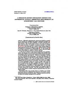
ˆ,C W Fig. 1. Linear systolic array for the feedback network

Combining (7) and (8), we can rewrite the output y(t) as yi (t) =

n


cij (t)xj (t) + fi,L (t),

f or i = 1, 2, . . . , n.

(9)

j=1

We have constructed a linear systolic array as shown in Fig. 1. This architecture consists of L+1 PEs. The PEs have the same structure, and the architecture has the form of a linear systolic array using simple PEs that are only conneted with neighboring PEs and thus can be easily scalable with more identical chips. ˆij,p (t) During p = 1, 2, . . . , L, the pth PE receives three inputs yj (t − p), w and fi,p−1 (t). Also, it updates PE cost fi,p (t) by (8). The L + 1th PE calculates

y1 (t) y2 (t) y3 (t) yn (t)

-z−1 -z−1 -z−1 -z−1 -z−1

? -y1 (t − 1) -y2 (t − 1) -y3 (t − 1) -yn (t − 1) -

w ˆn1,p

w ˆ21,p

w ˆ11,p

w ˆn2,p

w ˆ22,p

w ˆ12,p

w ˆn3,p

w ˆ23,p

w ˆ13,p

w ˆnn,p

w ˆ2n,p

w ˆ1n,p

6

6

×

-

+

- Register

-

Control

6

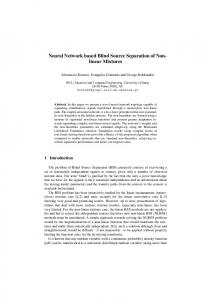
Fig. 2. The internal structure of the processing element

  R U

f1,p f2,p f3,p fn,p

A FPGA Architecture of BSS and Real Time Implementation

351

y(t) according to (9) using inputs x(t) and cij (t). In other words, we obtain the cost of PE using recursive computation. With this method, computational complexity decreases plentifully. The computational complexity for this architecture is introduced in the last subsection. The remaining task is to describe the internal structure of the processing element. Fig. 2 shows the processing element. The internal structure of the processing element consists of signal input part, weight input part, calculation part, and cost updating part. The signal input part and weight input part consist of the FIFO queue in Fig. 2, and take signal input y(t) and weight w(t) respectively. The two data move just one step in each clock. As soon as all inputs return to the queue, the next weight is loaded. When all the weights are received, the next input begins. The calculation part receives inputs y(t) and w at two input parts, then updates PE cost fi,p (t) according to (8). This part consists of adder, multiplier, and register. 3.2

Systolic Architecture for the Update

This section presents the architecture that updates the weights. This architecture also consists of the processing elements that operate in the same method. We define the processing element which the used in the update as the Update Element(UE). Efficient implementation in systolic architecture requires a simple form of the update rule. The learning algorithm of updating has the form wij,p (t) = wij,p (t − 1) − ηt f (yi (t))g(yj (t − p)), i, j = 1, 2, · · · , n, (i = j) p = 1, 2, · · · , L.

(10)

In this architecture, the function f (.) is used as the signum function f (yi (t)) = sign(yi (t)) and the function g(.) is used as the 1st order linear function g(yj (t)) = yj (t) because the implementation is easy with the hardware. Fig. 3 shows the systolic array architecture of the update process. If the number of signals is N , then the number of rows D is (N 2 +N )/2 . All arrays have the same structure and all weignts can be realized by using y(t) simultaneously. In a row in Fig. 3, if the number of PE is L, the number of columns is 2L + 1. In other words, the architecture of the update consists of D × (2L + 1) UEs. The cost of (d,p)th UE has the form ud,p (t) = ud,p (t − 1) − ηt f (yi (1/2(t − p − L)))yj (1/2(t + p − L)), d = 1, 2, · · · , D.

(11)

Fig. 4 shows the internal structure of the UE of the feedback network. The processing element performs simple fixed computations resulting in a simple design and low area requirements. The pth UE receives two inputs yi and yj , then one input becomes f (yi ). The cost of UE is added to the accumulated cost of the same processor in the previous step.

352

Y. Kim and H. Jeong

 -U ED,−L-

  -U ED,−p-

yN −1 (t)

? w(N −1)N,L

  - U ED,0 -

  -U ED,+p-

? w(N −1)N,0 ,? w(N −1)N,1 wN (N −1),0 wN (N? −1),1

 -U E2,−L-

 yN (t) -U ED,+L wN (N? −1),L

  - U E2,−p-

  - U E2,0 -

  - U E2,+p-

? w13,1

w13,0 ,? w31,0

? w31,1

  y3 (t) -U E2,+L

y1 (t)

? w13,L y2 ([ 12 (t

− 2L)])

 -U E1,−Ly1 (t)

y2 ([ 12 (t

y2 ([ 12 (t

− p − L)]) y2 (t − L)

  - U E1,−p-

y1 ([ 12 (t + p − L)]) ? w12,1

? w12,L

  - U E1,0 -

? w31,L + p − L)])

  - U E1,+p-

  y2 (t) U E1,+L -

y1 (t − L) y1 ([ 12 (t − p − L)]) y1 ([ 12 (t − 2L)]) ? ? w12,0 ,? w21,0 w21,1 w21,L

Fig. 3. Linear systolic array for update y1 (t − 1)

6

Z

−1

6 y1 (t)

-

ϕ(·)

f (y1 (t))

R 

y2 (t) · ηt

×

− +

up (t)

-

Z −1

-

up (t − 1)

+

6

? Z

−1

?

y2 (t − 1)

Fig. 4. The internal structure of update element

3.3

Overall Architecture

The system configuration is shown in Fig. 5. We observe a set of signals from an MIMO nonlinear dynamic system, where its input signals are generated from independent sources. The minimization of spatial dependence among the input signals results in the elimination of cross-talking in the presence of convolutively mixing signals. We assumed that auditory signals from n sources were mixed and reached n microphones far from the sources. The forward process of the feedback network algorithm uses two linear arrays of (L + 1) PEs. (nL) buffers are required for

A FPGA Architecture of BSS and Real Time Implementation

353

Unknown

si (t)

xri (t)

Convolutive mixing

sj (t)

-

xrj (t)

-

- yir (t) = F (si (t)) Forward process feedback network

- yjr (t) = F (sj (t))

6 6 6 6 6 w ˆ r−1w ˆ r−1

r−1 r−1 r−1 cij w ˆij,1 w ˆji,1

ij,L

ji,L

Weight

6

r−1 r−1 wij,0 wji,0

6

6 6 wr−1 wr−1 ij,L

ji,L

 Update feedback network



Fig. 5. Overall block diagram of feedback network architecture

output y(t) ,nL buffers for cost of PE, and (DnL) buffers for weight W (t). Since each output y(t) and weight W (t) are By bits and Bw bits long, a memory with O(nLBy + DnLBw ) bits is needed. Each PE must store the partial cost of Bp bit and thus additional O(nLBp ) bits are needed. As a result, total O(nL(By + Bp + DBy ) bits are sufficient. The update of the feedback network algorithm uses a linear array of D(2L+1) UEs. 2D(2L + 1) buffers are required for output y(t) and D(2L + 1) buffers for cost of UE. If UE stores the partial cost of Bu bits, total O(DL(4By + 2Bw )) bits are sufficient.

4

System Implementation and Experimental Results

The system is desiged for an FPGA(Xilinx Virtex-II XC2V8000). The entire chip is designed with VHDL code and fully tested and error free. The following experimental results are all based upon the VHDL simulation. The chip has been simulated extensively using ModelSim simulation tools. It is designed to interface with the PLX9656 PCI chip. The FPGA design implements the following architecture: – – – –

Length of delay: L=50 The number of input source: n=4 The buffer size for learning: 200 samples The learning rate: ηt = 10−6

As a performance measure, Choi and Chichocki [5] have used a signal to noise ratio improvement, SN RIi = 10 log10

E{(xi (k) − si (k))2 } . E{(yi (k) − si (k))2 }

(12)

354

Y. Kim and H. Jeong 4

2

0

−2

0

1000

2000

3000

4000

5000

6000

7000

8000

9000

0

1000

2000

3000

4000

5000

6000

7000

8000

9000

4

2

0

−2

Fig. 6. Two original speech signals 15 10 5 0 −5 −10

0

1000

2000

3000

4000

5000

6000

7000

8000

9000

−10 0

1000

2000

3000

4000

5000

6000

7000

8000

9000

15 10 5 0 −5

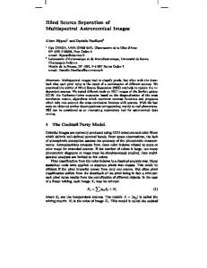
Fig. 7. Two mixtures of speech signals Table 1. The experimental results of SRNI with noisy mixtures SNR(signal to noise ratio)= 10 log10 (s/n) clean 10dB 5dB 0dB -5dB -10dB SNRI1(dB) 2.7061 2.6225 2.4396 2.3694 1.9594 0.1486 SNRI2(dB) 4.9678 4.9605 4.7541 4.6506 3.9757 3.2470

Two different digitized speech signals s(t), as shown in Fig. 6, were used in this simulation. The received signals x(t) collected from different microphones and recovered signals y(t) using a feedback network are shown in Fig. 7, 8. In this case, we obtained SN RI1 = 2.7061,and SN RI2 = 4.9678. We have evaluted the performace of the feedback network, given noisy mixtures. Table. 1 shows the experimental results of SRNI with noisy mixtures. The performance of this system measures were scanned for the SNR from -10dB to 10dB with an increment of 5dB. The system has shown good performance in high SNR (above 0dB only).

A FPGA Architecture of BSS and Real Time Implementation

355

10

5

0

−5

0

1000

2000

3000

4000

5000

6000

7000

8000

9000

0

1000

2000

3000

4000

5000

6000

7000

8000

9000

10 5 0 −5 −10

Fig. 8. Two recovered signals using the feedback network

5

Conclusion

In this paper, the systolic algorithm and architecture of a feedback network have been derived and tested with VHDL code simulation. This scheme is fast and reliable since the architectures are highly regular. In addition, the processing can be done in real time. The full scale system can be easily obtained by the number of PEs, and UEs. Our system has two inputs but we will extend it for N inputs. Because the algorithms used for hardware and software impelmentation differ significantly it will be difficult, if not impossible, to migrate software implementations directly to hardware implementations. The hardware needs different algorithms for the same application in terms of performance and quality. We have presented a fast and efficient VLSI architecture and implementation of BSS.

References 1. C. Jutten and J. Herault, Blind separation of source, part I: An adaptive algorithm based on neuromimetic architecture. Signal Processing 1991; vol.24, pp.1-10. 2. K. Torkkola, Blind separation of convolved sources based on information maximization. Proc. IEEE Workshop Neural Networks for Signal Processing 1996; pp.423432. 3. Hoang-Lan Nguyen Thi, Christian Jutten, Blind Source Separation for Convolutive Mixtures. Signal Processing 1995; vol.45, pp.209-229. 4. T. Nomura, M. Eguchi, H. Niwamoto, H. Kokubo and M. Miyamoto, An Extension of The Herault-Jutten Network to Signals Including Delays for Blind Separation. IEEE Neurals Networks for Signal Processing 1996; VI, pp.443-452. 5. S. Choi and A. Cichocki, Adaptive blind separation of speech signals: Cocktail party problem. in Proc. Int. Conf. Speech Processing (ICSP’97) August, 1997; pp. 617-622. 6. N. Charkani and Y. Deville, Self-adaptive separation of convolutively mixed signals with a recursive structure - part I: Stability analysis and optimization of asymptotic behaviour. Signal Processing 1999; 73(3), pp.255-266.

356

Y. Kim and H. Jeong

7. K. Torkkola, Blind separation of delayed source based on information maximaization. Proc. ICASSP, Atlanta, GA, May, 1996; pp.7-10. 8. K. Torkkola, Blind Source Separation for Audio Signal-Are we there yet? IEEE Workshop on Independent Component Analysis and Blind Signal Separation Aussois, Jan, 1999; France . 9. Aapo Hyvarinen, Juha Karhunen and Erkki Oja, Independent Component Analysis, New York, John Wiley & Sons, Inc., 2001. 10. K.C. Yen and Y. Zhao, Adaptive co-channel speech separation and recognition. IEEE Tran. Speech and Audio Processing 1999; 7(2),pp. 138-151. 11. A. Cichocki, S. Amari, and J. Cao, Blind separation of delayed and convolved signal with self-adaptive learning rate. in NOLTA,, tochi, Japan, 1996; pp. 229-232. 12. T. Lee, A. Bell, and R. Orglmeister, Blind source separation of real world signals. in ICNN,