Implementation of linear filters for iterative penalized maximum

606

EEE TRANSACTIONS ON NUCLEAR SCIENCE, VOL. 38, NO. 2. APRIL 1991

Implementation of Linear Filters for Iterative Penalized Maximum Likelihood SPECT Reconstruction Zhengrong Liang Department of Radiology, Duke University Medical Center Durham, North Carolina 27710

Abstract

11. THEORY Six low-pass linear filters applied in frequency space The log likelihood of a Poisson distributed photonwere implemented for iterative penalized maximum- detection process is well known [l-31: likelihood (ML) SPECT image reconstruction. The filters implemented were the Shepp-Logan filter, the Butterworth filter, the Gaussian'filter, the Hann filter, the ParZen filter, and where Y = {Ydf=l is the data vector with I elements, the Lagrange filter. The low-pass filtering was applied in fre- Q, = {$j& is the image vector of J elements to be reconquency space to projection data for the initial estimate and to structed, and Rij is the probability of detecting a photon emitthe difference of projection data and reprojected data for ted within pixel j and registered at detector bin i. In SPECT, higher order approximations. The projection data were the value of Rij depends on the deterministic effects of pixelacquired experimentally from a chest phantom consisting of projection geometry, photon attenuation and scattering, and non-uniform attenuating media. All the filters could collimation variations [6]. By use of Stirling's approximaeffectively remove the noise and edge artifacts associated tion, the likelihood function (1) becomes: with ML approach if the frequency cutoff was properly chosen. The improved performance of the M e n and Lagrange filters relative to the others was observed. The best This is the Kullback-Leibler information criterion [7] and has image, by viewing its profiles in terms of noise-smoothing, been widely used in information theory. edge-sharpening, and contrast, was the one obtained with the It has been recognized that the ML criterion [Eq.(l) or M e n filter. However, the Lagrange filter has the potential (2)] has the intrinsic instability of generating noisier images to consider the characteristics of detector response function. as the likelihood increases at higher iterations [3]. This instability associated with ML approach may be due to the neglect I. INTRODUCTION of the correlations among nearby pixels. A formal way to Quantitative single photon emission computed tomog- impose the correlations upon the ML approach is to carry out raphy (SPECT) has been limited mainly by the inadequate the maximum a posteriori probability (MAP) criterion by number of detected photons in projections. The projection specifying an a priori probability reflecting the correlations data contain Poisson noise associated with photon detection, via Bayesian analysis. attenuation and scattering effects of photons within the Let the log apriori probability of the correlations patient body, and the variations in collimator response with among nearby pixels be H (a), the log posteriori probability distance. The iterative maximum-likelihood, expectationis then: maximization (ML-EM) algorithm [ 1,2] provides a simple and accurate formula to compensate these effects. Although g(Q,)=L(YIQ,)+H(@). (3) the ML-EM algorithm can incorporate these effects in the Following the derivations given in [8], the solution which SPECTreconstruction (as well as the non-negativity of image maximizes g (0) is determined iteratively by: pixel values and the conservation of the acquired data), its neglect of correlations among nearby pixels may cause the noise and edge artifacts in the reconstructed images [3]. Moreover, the compensation during the reprojection and backprojection processes of the ML-EM algorithm is time consuming. The objective of this research was to implement the low-pass smoothing filters applied in frequency space [4,5] to alleviate the artifacts and reduce the computation where z k = & f ( @ ) / d $ k , 51")is an adjustable parameter, and time. i$'= $ ~ ) / ( 1 + 6 t ) Z k ) is the smoothed value of pixel k. The smoothing for $k is determined by the assumed apriori 1) ?his work was supported by Grant #HL44194, awarded by the correlations z k among nearby pixels. National Heart, Lung, and Blood Institute, and in part by Grant #CA33541, awarded by the National Cancer Institute and by Grant The difhulties with this formal MAP approach are the #DEFG05-89ER60894, awarded by the Department of Energy. specifications of an adequate prior z k and the adjustable parameter 51"). If an inadequate prior or adjustable parameter 0018-9499/91/0400-0606$01.000 1991 IEEE

607

is used, artificial biases and distortions are very likely to be generated in the reconstructed images [8]. Research for adequate priors and appropriate numerical methods has been an interesting topic in recent years [9-111. Perhaps an easier approach to penalize the ML estimation is to use spatial-domain, non-linear smoothing techniques [12]. The non-linear smoothing can be easily used to determine the $:") in Eq.(5). When applying this spatialdomain penalized ML approach of Eq.(5) to SPECT reconstruction, the computation burden for Rik (which contains attenuation, scattering, and collimation variation effects) during the reprojection and backprojection processes is very heavy. One way to reduce the computation time is to cut the compensating calculations during the backprojection using the filtered backprojection approach 151. Keeping this in mind, equation (5) can be reformed as:

the iterative penalized ML-EM algorithm (6). The filters implemented were the Shepp-Logan filter [16], the Butterworth filter [4], the Gaussian filter [17], the Hann filter [4], the Parzen filter [HI, and the Lagrange filter [19]. These filters are defined, in the field of reconstruction from projections, by the corresponding windows multiplied by the ramp function If I (f is the spatial frequency) [5]. The former five windows were described in detail in [5]. The Lagrange window is defined as: F ( f )=

1 1 +q(2Kf)4/ I M T F ~ ) P

(7)

where q is a parameter and MTF (f) is the Fourier transform of the detector response function. The value q = 5 was used. M T F ( f ) = exp [ - (112) U/fN)' ] was assumed [20]. fN is the Nyquist frequency. In the implementation,fN was defined by the unit of cycles lpixel and fN = 0.5 was then chosen. The parameter (2n) defined in the Butterworth window, I/[l+(f/fN)'"], was chosen to be 20 [5]. (When 2n = 8 was used, the resulting images were similar to those with where the first term on the right-hand side (RHS) is the 2n = 20). For the Gaussian window, exp [-IC (f/ o ) 3~ with smoothed estimate at the n-th iteration and the second term is o = 4 In (2)Ilc (FWHM)2, the parameter of full-wide-halfthe correction for the (n +l)th approximation. The term in maximum (FWHM) relating to detector resolution was the bracket of Eq.(6) represents the ratio of the contributions assumed to be 2 [5]. (When value 4 was used, similar results of a group of pixels around pixel k and all ixels to the were obtained). The parameter values chosen above have acquired datum Yi. The ratio Tik=Rik$k / x j R ~ $ ( " )been widely used, e.g., see [5,16-203. There is no parameter depends on the source distribution (Rik and a) and the in the other three windows. Two approaches in image space were used to calculate U riori information about the smoothing associated with the first term $:"' on the RHS of Eq.(6): one assumed a very $k * (n)An assumption is made that the ratio Tik represents a weak correlation among nearby pixels (i.e., $k ->@)), convolution operator. Mathematically the assumption is another used the edge-preserving smoothing [21] for a relaexpressed as Tik= T(i-k). This assumption is heuristc. tively strong correlation. Detailed discussion is beyond this paper. Since the smoothwas computed as follows [see The initial estimate ing in image space is desired for the convolution operator, the Eq.(5)]: First apply the chosen low-pass filter in frequency corresponding operator in frequency space would be a low- space to filter the acquired data ( Y i ) and then backproject the pass filter [4-51. Since the mapping of the smoothing from filtered data to image space. [The filtering and backprojecimage space to projection space is very difficult to formulated tion are the well known filtered backprojection method mathematically, the expression of the low-pass filter with the (FBP)]. Finally the backprojected image was divided by the desired smoothing property is not known yet. In this paper, normalization factors R i k } . In the implementation, these those low-pass filters of well known characteristics [4-51 are factors contain the information about the geometry between considered and compared for the purpose of alleviating the pixels and projections and the non-uniform attenuating proartifacts associated with the ML-EM algorithm. perties of a chest phantom from which the data were It is noted that a similar filtering approach has been acquired. The negative pixel values were either accepted or taken by Tanaka [13-151 to improve the performance of the forced to be zero for higher order approximations. This will ML-EM algorithm. Tanaka introduced two convolution be discussed later. operators of Eq.(20) in [13] to adjust the ratio of projection A fast non-uniform attenuated projector was used in data and reprojected data [ R;j $(")I at each iteration. computing the reprojected data [ C, Rij $(")) and the normaliSubstantial variations along the approach are presented in zation factors Rik}. The fast attenuated projector is simi[W. lar to the one described in [22]. The differences between them are: (i) the attenuation factor within each pixel is calcu111. METHODS lated by mass-center average in the fast projector and by Six low-pass linear filters applied in frequency space integral in [22]; and (ii) the intersecting lengths of pixels and were implemented to filter the frequency components of projection rays are computed by recursion in the fast projec[ Yi Rc ) in the second term on the RHS of Eq.(6) for tor and by forward tracing in [22]. As an example of projecting a 128 x 128 image array to 120 projections with 128 sam-

-8)

-8)

{xi

Yi/cj

x.

{xi

608

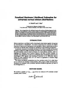
ples per projection, the fast attenuated projector took 33 seconds to finish the projecting process, while the projector of [221 needed 58 seconds. The 2-point interpolation backprojector [231 was used to backproject the filtered data Yi) for the initial estimate and ( q k ( Y i - x . RQ $$'")} for higher order approximations. Since the compensation of nonuniform attenuation was not involved in the backprojection, less computation time was needed. The interpolation backprojector uses the distance between the pixel center and the projection ray as the weight rather than the intersection length of the pixel and the projection ray (as the attenuated projector does). The chest phantom with non-uniform attenuating properties was an elliptical cylinder filled with water containing Within the elliptical cross section there were two regions of low density wood "lungs" and a region of nylon "bone" as shown by Fig.1. Both the lung and bone regions had zero activity. A hot sphere within the cylinder had approximately five times the concentration of Zlz3 as the water had. The non-uniform attenuating properties of the phantom were considered during image reconstruction process. The projection data were acquired at 120 projection angles equally spaced over 360 degrees by a three-headed SPECT system') with medium energy, parallel hole collimators. Each projection had 128 x 128 samples equally spaced. The projection slice through the center of the hot sphere had approximately half million counts and was used to reconstruct the 128 x 128 image array. Detailed information can be found in [24]. The attenuation map of the chest phantom was obtained by the uncompensated reconstruction from the acquired data and the known attenuation coefkients of the phantom. The evaluations at the performance of the low-pass linear filters were based on the horizontal and vertical profiles through the reconstructed images. The profiles were examined, by viewing, in terms of noise-smoothing, edgesharpening, and contrast between the regions of the lung, bone, hot sphere, and background.

acquired data after 20, 30, and 50 iterations are shown in Fig.2. After 20 iterations, noise and edge artifacts were present. Fig3 shows the images reconstructed using the penalized ML-EM algorithm to the acquired data. The SheppLogan filter with cutoff frequancy at half fN was used in frequency space for the second term on the RHS of Eq(6). The weak correlation was assumed for the first term on the RHS of Eq.(6). The top image was produced by backprojecting the filtered acquired data only (i.e., the result of FBP). The one on the second row was the initial estimate do). The image on the third row was obtained after one iteration. The bottom one was the result after 9 iterations. Similar images were obtained for the Buttetworth filter and the Gaussian filter. Therefore, these images are not presented here. The negative pixel values were accepted for the iteration process. Although this is not fit with the theoretical development of Eq.(5), it is interesting to see the effect on the reconstructed images (as addressed later). The reconstructed images with the Hann filter under the same condition as described in Fig3 are shown in Fig.4. Fig.5 shows the reconstructed images with the Parzen filter under the same condition of Fig.3. Similar results were generated when the Lagrange filter was used. Hence, these results are not presented here. All the frequency-space filters applied with the penalized algorithm could effectively remove the noise and edge artifacts if the frequency cutoff was properly chosen. When the cutoff frequency was set to fN, the resulted images were noisier. If the cutoff frequency was chosen at 0.25 fN, smoother images were obtained. By viewing all the horizontal and vertical profiles through the images, the Parzen filter (see Fig.5) showed the best performance on removing the artifacts among the six implemented filters. However, the Lagrange filter offers the potential to consider the detector response function. The effects of collimation variation and photon scattering may be considered via the detector response function, although the normalization factors ( R i k ) in Eq.(6) contain all the deterministic e f k t s during SPECT data acquisition. Although it is similar to the Wiener filter [25], the IV. RESULTS Lagrange filter is much easier to implement. Further study on In this a few images reconstructed by these two filters to consider the collimation and applying the penalized ML-EM algorithm(6) to the acquired photon is under progress. data from the chest phantom are presented. The profiles shown were drawn through the images at the positions indiSince the Metz filter [26] is strongly countdependent, cated. The difference of smoothing the first term 4); on the it is relatively difficult to apply it in frequency space to the RHS of &.(Q with weak and strong come~tionswill be difference of the acquired data and the reprojected data for me effect of accepting negative pixel values or the iterated solution. For the initial estimate, the Metz filter forcing them to be zero for higher order approximations has the potential to consider the effects of collimation variation and photon scattering [20]. be addressed. For comparison, the images reconstructed by applying When the iteration process generating the above the iterative unpenalized ML-EM algorithm [1,21 to the images continued beyond 9 iterations, the iterated images were noisier and noisier. This instability may be due to the 2) ' h e Triad SPECT system. assumption that the correlation in image space for the first

(ck

term $) on the RHS of Eq.(6) is very weak. The egdepreserving smoothing [21] which reflects a relatively stron -cnP correlation was then applied to determine the first term $k . The reconstructed images using the penalized algorithm (with the six low-pass filters applied in frequency space and the edge-preserving smoothing applied in image space) were similar to the corresponding images shown above before 5 iterations. Beyond 5 iterations, the generated images were stabilized. It concludes that the edge-preserving smoothing is necessary. Under this conclusion, the smoothing in image space is consistant with that in projection space. As an example, Figs.6 and 7 show the images obtained using the penalized algorithm with the Parzen and Lagrange filters after 10,20,50,and 100 iterations under the same condition as described in Fig.3, except that the first term on the RHS of Eq.(6) was computed by the edge-preserving smoothing. The penalized algorithm was run up to 200 iterations. At higher iterations, only the negative pixel values changed a somewhat degree. This small effect was due to the acceptance of the negative values during iterations. It also caused small variation in the total counts of projection data after each iteration. By forcing the negative values to be zero, the iterated images after 10 iterations were similar to the 10th iterated image and the total counts after each iteration were conserved. Therefore, it is recommended that the negative pixel values are set to zero during iteration process. By forcing the negative values to be zero, the implementation of the algorithm (6) as shown above is fit with the theoretical development of Eq.(5).

$'

V. CONCLUSIONS We have implemented six low-pass linear filters applied in frequency space for the iterative penalized ML-EM algorithm (6). The implementation requires: (i) an edgepreserving smoothing is necessary for the first term $) on the RHS of Eq.(6); (ii) the negative pixel values would be set to zero during iteration process. The SPECT images were reconstructed using experimentally acquired data from a chest phantom consisting of non-uniform attenuating media. All the filters stabilized the iterated reconstructions and no stopping criterion is needed. The noise and edge artifacts associated with the ML-EM algorithm could be removed if the cutoff frequency was properly chosen. The improved performance of the Parzen and Lagrange filters relative to the others was observed. The best image, by viewing its profiles in terms of noise-smoothing, edge-sharpening, and contrast, was the one obtained with the Parzen filter. However, the Lagrange filter has the potential to consider the characteristics of detector response function. Although the formal way of specifying an apriori correlation prior for the MAP solution is desired, the frequency-domain filtering approach is easier to implement. The advantage of computation will be accentuated when the effects of collimation variation and photon scattering are necessary.

VI. ACKNOWLEDGEMENT The author is grateful to Dr.Ronald Jaszczak and Dr. Dave Gilland providing valuable comments on this paper. Mi. Kim Greer assisted with the data acquisition. VII. REFERENCES 111:

L. Shepp and Y. Vardi, "Maximum Likelihood Reconstruction for Emission Tomography." IEEE Trans. Med. Imaging, vol.1, pp.113-122, 1982.

PI:

K. Lange and R. Carson, "EM Reconstruction Algorithms for Emission and Transmission Tomography." J. Comput.

Assist. T o m g . , ~01.8,pp.306-316, 1984. 131: D. Snyder, M. Miller, L. Thomas and D. Politte, "Noise and Edge Artifacts in Maximum-Likelihood Reconstruction for Emission Tomography." voI.6, pp.228-238, 1987.

IEEE Trans. Med. Imaging,

Digital Filters, Prentice-Hall, Inc., NJ,

PI:

R. Hamming, 1983.

151:

G. Gullberg and T.Budinger, "The Use of Filtering Methods to Compensate for Constant Attenuation in Single Photon Emission Computed Tomography." IEEE Trans. Biomed. Engin., ~01.28,pp.142-157, 1981.

161:

Z. Liang, R. Jaszczak, C. Floyd, et al, "Reprojection and Backprojection in SPECT Image Reconstruction." Proc. IEEE, Energ. Inform. Tech. Southeast, pp.919-926, 1989.

171:

S . Kullback and R. Leibler, "On Information and Sufficiency." Ann. Math. Statist., v01.22, pp.79-86, 1951.

181:

Z. Liang, R. Jaszczak and K. Greer, "On Bayesian Image

PI:

Reconstruction from Projections: Uniform and non-uniform a priori source information." IEEE Trans. Med. Imaging, voI.8, pp.227-235, 1989. S . Geman and D. Geman, "Stochastic Relaxation, Gibbs Distributions, and the Bayesian Restoration of Images." IEEE Trans. Part. Analy. Mach. Intel., ~01.6,pp.721-741, 1984.

[lo]: J. Besag, "On the Statistical Analysis of Dirth Pictures." J. R. Statist. Soc., v01.48, pp.259-302, 1986. [ll]: S . Geman and D. McClure, "Statistical Methods for Tomographic Image Reconstruction." Bull. ISI, ~01.52,pp.5-21, 1987. [12]: R. Chin and C. Yeh, "Quantitative Evaluation of Some Edge-Preserving Noise-Smoothing Techniques." Computer Vision, Graphics, Image Proc., vo1.23, pp.67-91, 1983. [13]: E. Tanaka, "A Fast Reconstruction Algorithm for Stationary Positron Emission Tomography Based on a Modified EM Algorithm." IEEE Trans. Med. Imaging, voI.6, pp.98-105, 1987. [ 141: E. Tanaka, "A Filtered Iterative Reconstruction Algorithm for Positron Emission Tomography." in Information Processing in Medical Imaging. Plenum Publishing Corp., pp.217-233, 1988.

[15]: E. Tanaka, "Intelligent Iterative Image Reconstruction with Automatic Noise Artifact Suppression." Presented at IEEE 1990 Medical Imaging Conference, Arlington, VA, USA.

610

[16]: L. Shepp and B. Logan, "The Fourier Reconstruction of a Head Section." IEEE Trans. Nucl. Sci., v01.21, pp.2143,1974. "The Exponential Radon [17]: 0. Tretiak and C. Metz, Transform." SIAM J . Appl. Math., vo1.39, pp.341-354, 1980. [18]: E. Parzen, "Mathematical Considerations in the Estimation of Spectra." Technometrics, vo1.3, pp.167-190, 1961. [19]: D. Phillips, "A Technique for the Numerical Solution of Certain Integral Equations of the First Kind." J . Assoc. Compur. Mach., vo1.9, pp.84-97, 1962.

[20]: M. King, R. Schwinger, B. Penney, et al, "Digital Restoration of Indium-111 and Iodine-123 SPECT Images with Optimized Metz Filters." J . Nucl. Medicine, vo1.27, pp.1327-1336, 1986. (211: 2. Liang, R. Jaszczak, C. Floyd and K. Greer, "A Spatial Interaction Model for Statistical Image Processing." in Information Processing in Medical Imaging. WileyLiss, New York, pp.29-43, 1990. [22]: G. Gullberg, R. Huesman, J. Malko, et al, "An Attenuated Projector-Backprojector for Iterative SPECT Reconstruction." Med. Physics, ~01.30,pp.799-815, 1985. ~ 3 1T. Peters, "Algorithms for Fast Back-and-Reprojection in Computed Tomography." IEEE Trans. Nucl. Sci., ~01.28, pp.3641-3647, 1981.

Fig.2: The images reconstructed by applying the iterative unpenalized ML-EM algorithm to the projection data acquired from the chest phantom. The top one was generated after 20 iterations. The image on the second row was obtained after 30 iterations. The bottom image was the result after 50 iterations. The curves are the profiles each through the center of the images horizontally at the indicated positions.

[241 D. Gilland, R. Jaszczak,K. Greer and R. Coleman, "Quantitative SPECT Reconstruction of Iodine-123 Data." J . Nucl. Medicine, vo1.31, 1991, in press. [25]: W. Pratt, "Generalized Wiener filtering computational techniques." IEEE Trans. Computer, v01.21, pp.636-641, 1972. [26]: C. Metz and R. Beck, "Quantitative Effects of Stationary Linear Image Processing on Noise and Resolution of Structure in Radionuclide Images.'' J. Nucl. Medicine, vo1.15, pp.164-170, 1974.

1 ~ 8 .cm+l 8

I 1-29.9

ctn

I *I

Fig.1.: The cross-section of the chest phantom.

Fig.3: The images reconstructed using the penalized M L EM algorithm with the Shepp-Logan filter at cutoff frequency of 0.5 f , . The weak nearby correlation was assumed. The top image was produced by backprojecting the filtered projection data only. The one on the second row was the initial estimate. The image on the third row was obtained after one iteration. The bottom one was the 9th iterated result. The profiles were drawn through the images three pixels below the image center.

61 1

Fig.4: The reconstructed images using the penalized algarithm with the Hann filter in the same situation as described in Fig.3.

Fig.6: The images obtained using the penalized algorithm with the Parzen filter after 10, 20, 50, and 100 iterations under the same condition of Fig.3, except that the relatively strong correlation was assumed.

Fig.5: The reconstructed images using the penalized algorithm with the Parzen filter under the same condition of Fig.3.

Fig.7: The images obtained using the penalized algorithm with the Lagrange filter after 10, 20, 50, and 100 iterations under the same condition of Fig.3, except that the relatively strong correlation was assumed.