Implementation of Pulse-Coupled Neural Networks in a ... - CiteSeerX

Implementation of Pulse-Coupled Neural Networks in a CNAPS Environment

Jason M. Kinser Thomas Lindblad Royal Institute of Technology

Pulse coupled neural networks or PCNNs are biologically inspired algorithms very well suited for image/signal pre-processing. While several analogue implementations are proposed we suggest a digital implementation in an existing environment, the CNAPS or Connected Network of Adapted Processors System The reason for this is two fold. Firstly, CNAPS is a commericially available chip which has been used for several neural network implementations. Secondly, the PCNN is, in almost all applications, a very efficient preprocessor requiring subsequent and additional processing. This may include gating, Fourier transforms, neural classifiers, data mining, etc, with or without feedback to the PCNN.

pulse coupled neural networks, image/signal pre-processing, segmentation, edge detection, object isolation

The present work is carried out under contract (93:400) with the Swedish Research Council for Engineering Sciences (TFR). One of us (JMK) would also like to acknowledge a fellowship from the school of engineering physics at KTH. We acknowledge discussions with D. Hammerstrom, Werner Salmen and Michel Sincovicz of Adaptive Solutions, Inc and Cromemco, GmbH, respectively.

1. INTRODUCTION There are several advantageous with analogue implementations of neural networks. The main one is, of course, that most signal sensors generate analogue signals. Several years ago Intel introduced the Electrically Trainable Neural Network, ETANN i80170NX [1-4], with a fairly conventional back-propagation (BP) algorithm and a processing time of a few micro seconds. The main disadvantageous of the analogue implementations are the relatively low precision (12 %), the sensitivity to noise and the fact that one generally requires some post-processing of the outputs from the neural networks. This is generally performed using some von Neumann computer, i.e a digital machine. Pulse Coupled neural Networks, PCNN, [5-10] could easily be implemented as hybrid circuits, i.e. an analogue input and a digital output. One would simply have an analogue input to the circuit and make use of the inherent feature that the output is a temporal series of binary images. However, as has been shown in several applications [8-14], the PCNN is “only” a preprocessor requiring subsequent processing. This post-processing may be carried out in several steps and include gating the output, Fourier transforms, etc, generally with feedback to the PCNN [15-19]. Other means of post-processing may include the use of other types of neural networks including BP [20], DDA/RBF [21], ART [22], for classification and identification. The PCNN algorithms also have several parameters which it may be desirable to change during the adaptation to the particular input. The CNAPS or Connected Network of Adapted Processors [23] system is NOT a generalpurpose parallel architecture, but one which has been optimized for pattern recognition and signal processing. The system is based on a single-instruction, multiple-data (SIMD) computer, i.e. each processing node (PN) acts on its own slice of data, but all active PNs execute the same instruction at the same time. In this investigation we have used a PCI card with 8 chips, each with 16 processors for a total of 128 PN. The CNAPS system involves an programming environment that includes its own C and Assembler languages plus an application interface (CNapi). This means that implementations can be made fairly fast and efficient and evaluated and modified at will. The inclusion of post-processing and dynamic communication between processing steps could be added, tested evaluated and changed as needed. Of course, we also expect the code to run faster in the parallel processing environment. The present paper describes the first implementation of the PCNN in the CNAPS. A brief resume of the PCNN and some details of the CNAPS are given in the next two chapters. These sections are followed by some details on the implementation and its evaluation. We conclude the paper by suggestion on implementations of post-processors and future work on full systems implementations.

2. THE PCNN AND ITS INHERENT FEATURES The PCNN is a digital simulation of the cat’s visual cortex. It generates a sequence of binary images containing segments and edges of the input scene. It operates by iterating the following equations Fij[n] = exp(-αF) Fij[n-1] + VF Σ mijkl Ykl[n-1] + Sij

(1)

Lij[n] = exp(-αL) Lij[n-1] + VL Σ wijkl Ykl[n-1],

(2)

Uij[n] = Fij[n] (1 + β Lij[n]),

(3)

Yij[n] =

{

1 if Uij[n] > Θij[n] and

(4)

0 otherwise

Θij[n] = exp(-αΘ) Θij[n-1] + VΘYij[n-1].

(5)

Here S is the input stimulus (e.g. the intensity of pixel i,j), F is the feeding portion of the neuron, L is the linking, U is the internal activity, Y is the output and Θ is the dynamic threshold. The interconnections in m and w are local Gaussians (dependant on the distance between the neurons). These matrix elements are generally set equal in algorithmic implementations (although there are biological evidence for m ≠ w ). There are three potentials, V, and three decay constants α, associated with F, L and Θ, respectively. We also define a time signal as G[n] = Σ Yij[n],

(6)

The time signal, or the pulse integration signal, is thus simply the number of “on pixels” in each iteration. For simple inputs it becomes repetitive after a certain number of iterations, while for more complex inputs this does not seem to happen. Clearly the time signal would be very attractive to use in view of its simplicity. Except for the stimulus, S, (and sometimes the threshold Θ) the initial values are generally set equal to zero. This means that in the first iteration U = β and all neurons will output a “1”, or “pulse”. After the pulse, the dynamic threshold is raised by a large value VΘ. The internal activity values will reach a somewhat stable level and threshold will decay until once again the internal activity is greater than the threshold. Then again the neuron pulses and the threshold is raised significantly. Thus we reach a situation where the neurons have a periodic pulsing behavior. The local connections mentioned above, allow neighboring neurons to encourage each other to fire. This happens if the neurons have similar internal activity levels close to the threshold levels. Thus neurons with similar stimulus inputs tend to pulse in unison. This is the foundation of the segmentation feature of the PCNN. Once a region has pulsed, the neurons along the perimeter of the segment encourage the neighboring neurons which did not previously pulse to do so. In the next iteration the neurons neighboring the edge of the segment will pulse. This is

the foundation of the edge detection. As the PCNN progresses the thresholds of a segment, which have just pulsed, will eventually have decayed to a level that allows the same neurons to pulse again. However, due to the input intensities and different regional activities, the neurons within this segment may pulse in a sequence of frames. The segmentation now breaks up dependant on the texture of the input. The PCNN has been applied in various manners in order to make use of the intrinsic features mentioned above. This includes systems for image de-noising, image segmentation [10], static and dynamic object isolation [8,17], foveation [11], image fusion [18] and logical operations [23-25] including a solution to the NPC problem [26]. However, all these implementations requires some post-processing of the outputs of the PCNN. In fact, the PCNN is just a preprocessor which generates signals for further processing. This processing may include feedback to the PCNN. A simple, but typical, example is the de-noising. There are several ways to implement this, but one way is to modulate the output Y by replacing it with Y ‘ = Y(1 + cos(n/ 16)) in the equations above. Other post-processing approaches may include gating, Fourier transforms, etc. One may also consider comparing outputs with lookup tables, feeding outputs to other neural networks for classification (ART1) and identification. In fact, the PCNN may end up as a small but important part of a larger system designed for one or several of the aforementioned tasks. Still other implementations of the PCNN may require direct modifications of the equations above. This is the case for de-noising using the fast linking concept. The fast linking involves inserting and iterating the following U i[n’]= Fi[n’]( 1 + β(Σ wijkl Ykl[n’]))

Yij[n’] =

{

(7)

1 if Uij[n’] > Θij[n’] and

(8)

0 otherwise

until the output does not change (cf. also the appendix). The post-processing, the feedback of modified signals as well as changes of the original equations to achieve segmentation, etc, require fast and efficient implementation, testing and

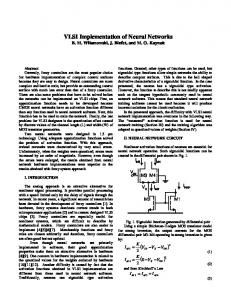
Figure 1. The architecture of the CNAPS

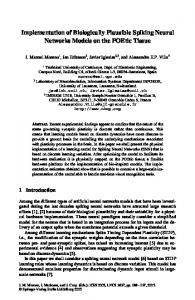
Figure 2. A block diagram of the CNAPS PCI board used in the present investigation. Note the connector to the mezzanine board and its use as discussed in the end of the paper.

evaluation. This is the other major reason for implementing the PCNN in an existing digital chips like the CNAPS. Systems may be developed and tested in a simple and convenient PC environment for embedded solutions. 3. THE CNAPS CNAPS stands for Connected Network of Adaptive Processors and is a multiprocessor chip. All processors receive the same instruction which they mandatory execute. This type of architecture is referred to as a single-instruction, multiple-data (SIMD) computer. Systems may be build using the CNAPS-1016 or CNAPS-1064 chips, having 16 or 64 processing nodes (PNs), respectively. Several chips may be cascaded so that a CNAPS Sequencer Chip (CSC) sequences instructions as well as data for all the chips. Each PN is a fixed-point processor with its own on-chip memory, registers and memory addressing unit. It has a multiplier, an adder/ subtracter (32-bit), a shift/logic unit and uses fixed-point, two’s complement arithmetic. An 8x8 or 8x16 (16x16) multiply is claimed to take one (two) clock cycle(s). Note that frequently employed operations like divide, squareroot and exponential have to be dealt with by the user for implementation of the paradigm. The CNAPS architecture is shown in fig. 1. As mentioned, and as can be seen from fig. 1, several PNs may be connected to each other and to the CSC. This is accomplished over three global buses: the command or interconnect bus, the input bus and the output bus. Each PN is also connected, by two 2-bit inter-PN buses, to its neighbors. The PNs have their own 4KB of on-chip memory and can perform 1-, 8-, or 16bit integer arithmetic. The clock frequency is 20 MHz and a multiply-and-accumulate operation can be performed in one clock cycle. The CSC ASIC chip controls the operation of the PN array as well as broadcasting data over the input bus and reading the results from the output bus. Other I/O modes are available in which the file memory and/or the CSC are bypassed to yield high aggregate throughputs. The CSC includes an ALU, and other features as described in the data book [19]. There are several commercially available systems based on the VME, ISA and PCI buses. In the present investigation we have used the CNAPS/PCI-DLX board [19] with eight 1016 chips, i.e a total of 128 PNs. The card, shown in fig. 2, is a full length card and plugs into a 32bit PCI single slot, but has a piggyback PCB with DRAM (SIMM socket). Operating at 20 MHz

Figure 3. The SAAB JAS 39 Gripen aircraft as an input to the PCNN and the pertinet outputs are shown here.

Figure 4. The input image of an aircraft flying upside down in front of a mountain side is shown in the top left image together with the output of a PCNN.

it is claimed to yield up to 2.56 billion multiply/accumulate (MAC) operations per second. One important feature of this card is the possibility to add an application-specific daughter card referred to as the mezzanine board. This could be used for high speed I/O and bypassing the PCI bus. The mezzanine board may also hold a post-processor, e.g. a FFT engine, a neural network chip, etc. The CNAPS-C language has features for parallel processing. Variables that are to reside on all processors are declared as poly type and code that will run simultaneously on each processor is declared within a domain. Some C features such as conventional floating point and long (4 byte) types are missing. Only 1 and 2 byte variables can be declared. In place of floating point variables, the CNAPS provides scaled variables, of one or two bytes, in which a fixed point can be set at a given bit to separate the whole number part from the fraction. Choosing the fixed point position is an important consideration. A low fixed point reduces the precision, whereas a high fixed point to achieve greater precision may result in overflows of the whole part. CNAPS programs often have multiple scaled variables with different fixed points to be used where greater or less fractional precision is necessary. The CNAPS processing elements (PE) were made as simple as possible. They can carry out the fast multiple and accumulate operation that is the key operation of most neural network algorithms, while e.g. the divide operator has to be

provided by the user. The reader is referred to the user ’s manuals and reports on recent implementations of DDA/RBF [20] and ART1 [21]. 4. THE IMPLEMENTATIONS 4. 1 General considerations The first code to be implemented was the Eckhorn model as described by equations, (1) (5). The input is an image of 128 x 128 which means that each PN is responsible for the calculations of 128 neurons. For the most part implementation of the PCNN in the CNAPS architecture was straight forward. There were a few changes that are addressed in this section, while further details are given in the appendix. In the CNAPS real numbers are represented by a scaled type. The scaled value requires the user to define the number of bits that will represent the integer part of the real number and the number of bits that will represent the decimal portion of the number with the total number of bits being 16 or less. Since this is not the mantissa/exponent representation the dynamic range of the scaled type is quite limited. Since the PCNN has decays which are term between 0 and 1, and since the integer did not have a divide function it became necessary to use this scaled type. The first concern is the dynamic range of each term of the computations. The largest value is VΘ which is 20 the term VΘ * Yij can become larger than 32. So there needs to be at least 6 bits to represent the integer portion of the real number. The smallest value of any significance is beta which is 0.1. This requires at least 4 bits but representation is much better with 6 or more bits. Since a total of 16 bits is allowed the PCNN fits comfortably within these parameters. The PCNN was first implemented using the standard library of the PCNN C-compiler, which resulted in a code performing only slightly (25%) faster than a 90 MHz Pentium PC. The main difficulty was to perform calculations of Σkl mijkl Ykl , etc. However, following suggestions from Adaptive Solutions and employing new/extra routines taken from their intlib library the code was rewritten as shown in the appendix. In this way we reached a “reasonable” speed of more than ten times that of the Pentium PC.

Figure 5. Example of de-noising using PCNN fast linking and gating. The image to the left is the input, the one in the middle is the time signal, while the de-noised image is shown to the right.Gating parameters (see text) are: start =9,

Figure 6. Example of results from a PCNN with a FPF postprocessor as discussed in sect. 4.5. The input is the image of fig 4. Three different masks are shown together with a cuts in the correlation matrix. The top row uses a “hand-tailored” mask and yields a strong correlation. A more “diffuse” mask (second and third row) will still yield strong correlations, in particular if several images are considered.

4.2 The implementation of the original PCNN The code is compiled using the CNAPS-C (with a command line: cnc -128 -g pcnn.cn) and executed from the CNAPS debugger by sourcing the following a script that: (i) initializes the arrays and make sure they all are zero, (ii) loads a file with the input stimulus (unsigned byte per pixel), (iii) the actual PCNN code (NITER determines the number of iterations) and (iv) writing the binary output images to the hard disk. Figure 3 and 4 show some examples of the outputs following two different inputs. The first example includes the well-known JAS 39 Gripen fighter over the Stockholm archipelago and the aircraft is easily seen in the output. The second example (fig. 4) involves a plane flying upside down with some mountains in the background. Here it is even hard to see the plane in the original image, the input. Nevertheless, the wings and other parts are identified in the output. 4.3 Implementation of a fast linking PCNN The second implementation deals with one of the methods of de-noising the original image. The fast linking PCNN computes the feeding, linking, internal activity and the pulse as does the “usual” or Eckhorn PCNN as described in eqs (1-5). Then it repeats computations of the convolution, the internal activity and the pulse until the pulse remains constant, cf. eqs (8)-(9). Then it computes the threshold. The logic of this system is that the linking waves are allowed to “travel” far beyond the limited range of the Eckhorn model. It is inherent of the fast linking approach that it computes slower. Fast linking was applied to a typical high energy physics situation, i..e. some 2-D Gaussian peaks and some noisy background. This is a situation where other methods have turned out not to work so well.

4.4 Implementation of a gated PCNN The third implementation of the PCNN uses time signal to determine which pulse output images are to be accumulated. There are several differences between this and the original implementation. Thus there are three new variables that deal with the gating operation. The first is StartGate which indicates the number of iterations that will pass before the accumulation begins. The second is OpenGate which indicates the number of iterations that the gate will open. The third is CloseGate which indicates the number of iterations for which the gate will be closed. The system will go StartGate iterations, open the gate and then alternate OpenGate and CloseGate. The other major difference originates from requirement of local memory on the CNAPS. Each PN has 4 K of memory, which is not enough to store also the accumulation array. Pulse integration has been proposed for data compression and platonic icon generation [23]. Gating of this pulse integration signal was also added to the parallel PCNN program. It can be explained by the following example. Consider the input in fig. 5 (left) which has two events that are to be isolated by the PCNN. Using fast linking the noisy background which would normal pulse in several PCNN iterations now pulses in a single iteration. The pulse integration or time signal is shown in fig. 5 (middle). Noting that the background pulses occur periodically it then becomes quite easy to accumulate Y only during iterations in which the background does not pulse. This is done by simply gating the accumulation. The final output is shown in fig. 5 (right). Again, this code required only a few extra controls and the accumulation of the Y so the code can remain quite parallel. 4.5 Implementation of a PCNN with a post-processor Finally, a Fractional Power Filter (FPF) [12,27] was employed as a postprocessor to analyze the pulse outputs. The FPF is a trainable composite filter that can manipulate the trade-off between generalization and discrimination that is inherent in first order systems. The FPF has a user defined parameter to control the range of generalization to discrimination. It turned out that the FPF could not be implemented in the CNAPS due to lack of memory and precision. However, as will be discussed below, one may implement a FFT hardware (in the present case a 2-D FFT with a Kaiser window was used) on the mezzanine board of the CNAPS. This will most likely solve the problem and speed up the computation as well. In the present work we implemented the FPF postprocessor in the Pentium. The FPF was trained on a single pulse image (with all nontarget pulses removed) and a slice of the correlation with pulse frame is shown in the top row of fig.6. Other FPFs were constructed manually (no pulse images were used) in order to show the robust quality of this detection system. These examples are included in fig. 6. Side lobes in some correlation plots can be quite significant. However, the accumulation of correlations maintain a high quality of the target peak and also diminish the effects of the side lobes due to their stochastic nature [17].

5. FUTURE DEVELOPMENTS As mentioned previously, the PCNN is an excellent preprocessing device, but it generally requires application-dependant post-processing algorithm(s) for the individual applications. Implementing the PCNN in CNAPS makes it possible to add such post-processing with or without feedback. We will use the previously implemented ART1 and DDA/RBF algorithms for post-processing which involves classification and recognition. Other ongoing projects include the use of wavelet transforms and data mining combined with neural assimilation of the mined fragments. The use of a combinatorial approach to pattern identification could often be very rewarding. The TOTEM chip has been developed at Trento [33] and tested with satellite image data as well as HEP data [28-30]. Implementing the TOTEM chip on a mezzanine card (cf. fig. 2) is one way to add an efficient postprocessor. In several application the preprocessing simply involves the extraction and/or enhancement of the input signal, which then needs to be compared and identified using a data base. Data mining is a relatively new concept and we have recently been evaluating a hardware implementation [31] for exact as well as homology searching. An implementation of a hardware search engine on a mezzanine card is suggestive for future research. The enhancement of the signal performed by the PCNN preprocessor can be used to group together objects having similar characteristics. This can be achieved by means of neural clustering [32] as well as other techniques. 6. SUMMARY In the present paper we have showed that the CNAPS can hold the PCNN in several versions. The algorithm also runs 10 - 15 times faster as compared to implementations in a 90 MHz Pentium PC. However, this is not the main reason for choosing the CNAPS even if speed is of importance. The main reasons are the existence of the CNAPS as a commercially available circuit with tools for application developments and the fact that post-processing algorithms (FFT, ART, BP, DDA/RBF, etc) can be added. Another important reason during the development of an embedded solution is the mezzanine card, which can hold other specific circuits as discussed in the previous section. This piggyback implementation may include specific VLSI circuits for FFT or data mining as well as any of the few neural network chips available today [26]. References [1] [2]

[3]

80170NX Electrically Trainable Analog Neural Network, Intel Corp. Santa Clara, CA, Feb. 1991 B. Denby, Th. Lindblad, C. S. Lindsey, Geza Szekely, J. Molnar, Åge Eide, S.R. Amendolia and A. Spaziani, Investigation of a VLSI neural network chip as part of a secondary vertex trigger Nucl. Instr. Meth. A335 (1993) 296 - 304 P. Hörnblad, Thomas Lindblad, Clark S. Lindsey, Géza Székely and Åge Eide, Filtering data from a drift-chamber detector using neural networks, Nucl. Instr. Meth. A336 (1993)

[4]

[5] [6] [7]

[8] [9] [10] [11] [12] [13] [14] [15] [16] [17] [18] [19] [20] [21]

[22] [23] [24] [25] [26] [27]

285-290 T. Akkila, T. Francke, Th. Lindblad and Å. Eide, An Analog Neural Network Hardware Solution to a Cherenkov Ring Imaging Particle Identifier, Nucl. Instr. Meth. A327 (1993) 566-572 J.L. Johnson, Pulse-Coupled Neural Nets, translaton, rotation, scale and intensity signal invariances for images, Appl. Opt. 33(26) pp 6239-6253 (1994) J.L. Johnson, Pulse-Coupled Neural Networks, Proc. NNW, Ablex Publ. Corp. & Critical Reviws Vol CR55 p. 47-76 J.M. Kinser,Recent Research in Pulse-Coupled Neural Networks,International Conference on PCNN, MICOM, Huntsville, AL, and A Simplified Pulse-Coupled Neural Network, SPIE Vol 2760, pp. 563-567 Jason M. Kinser, Dynamic Object Isolation, submitted to J. Artificial Neural Networks H.S. Ranganath and G. Kuntimad, Image Segmentation using Pulse Coupled Neural Networks, IEEE (1994) 1285-1290 H.S. Ranganath and G. Kuntimad, Iterative segmentation using Pulse coupled neural net works, SPIE volume 2760, p. 543-554 Jason M. Kinser, Foveation by a Pulse-Coupled Neural Network, in manuscript Jason M. Kinser,Parameter Esitmation Using Dual Fractional Power Filters, in manuscript Jason M. Kinser and John L. Johnson,Object Isolation, Optical Memories and Neural Nets 5(3) 1996 Vlatko Becanovic, Diploma work, KTH, Stockholm, Sept. 1996, TRITA-FYS-9041 Th. Lindblad, C.S. Lindsey and V. Bekanovic, Intelligent detectors modelled from the cat’s eye AIHENP'96, Lausanne, and to be published by World Scientific Th. Lindblad and J.M. Kinser, Inherent properties of wavelet transforms and pulse coupled neural networks, this issue J.M. Kinser, J.L. Johnson, Object Isolation, Optical Memories and Neural Networks 5(3) 1996 J.M. Kinser, Multi-spectral Object Isolation, Opt. Eng., submitted Adaptive Solutions Inc, http://www.asi.com Jason Charles Browne, High Speed Image Information Extraction Using Semiconductor Nased Neural Networks, Master Thesis, SINTEF and University of Oslo, 1996 Th. Lindblad, G. Székely, Mary Lou Padgett, Å J. Eide and C. S. Lindsey, Implementing the Dynamic Decay Adjustment Algoritm in a CNAPS parallet Computer System. Nucl. Instr. Meth. in press C.S. Lindsey and Th. Lindblad, Unsupervised Learning with ART on the CNAPS, AIHENP'96, Lusanne Sept. 1996 and to be published by World Scientific J.M. Kinser, Syntactical Computing using PCNN Modules, Proc. SPIE, Denver, CO, 1996 J.M. Kinser, J.L. Johnson and H.J. Caulfield, Synergetic Pulse-Coupled Nerural Network Pattern Recognition, Optical Memories and Neural Networks 5(3) 1996 J.M. Kinser and H.J. Caulfield, O(No) Pulse-Coupled Neural network Performing Human-Like Logic, Proc SPIE 2760 555-562 (1996) H.J. Caulfield, J.M. Kinser, manuscript 1996 J.D. Basher and J.M. Kinser, Fractional-Power Synthetic Discrimainant Functions, Pattern Recognition, 27 (4) 577-585 (1994)

[28] R. Johansson, Diploma Work, KTH Sept 1996, TRITA-FYS-9040 [29] Clark S. Lindsey and Thomas Lindblad, Experience with the Reactive Tabu Search as Implemented in the Totem Chip, ICNN'96, Washington DC, June 1996 [30] Å. Eide, R. Johansson, Th. Lindblad and C. S. Lindsey, Data Mining and Neural Networks for Knowledge Discovery, AIHENP'96, Lusanne and to be published by World Scientific [31] Clark S. Lindsey and Thomas Lindblad, Review of Hardware Neural Networks: A User's Perspective, Int. Journal of Neural Systems, Vol 6 (Supp 1995) 215-224, ISBN 981-02-2491-5 [32] IBM QUEST Data Mining Project and the IBM Intelligent Miner, WWW-pages [33] A. Sartori, G. Tecchiolli, C. Mezzena, Totem PC ISA Board, Technical Reference Manual, ISN Trento, Rev. 1.0 August 1995

Appendix - Details on implementation The CNAPS board used 128 parallel PEs. Each PE had 4K of local RAM. This was sufficient to process 128 x 128 neurons with each PE computing for 128 neurons. The local memory was sufficient to hold 128 elements for each array, S, F, L, U, T, and Y. Extra space was also required to store the convolution result Q and outputs from neighboring neurons. The convolution kernel K was stored in mono memory since it was constant and common for all PEs. The declaration for NODES = 128 neurons is domain neuron { sval F[DIM], L[DIM], U[DIM], T[DIM], Y[DIM], S[DIM], W[DIM]; sval YK[M]; } node [NODES];

where sval represented the real number type and DIM = 128 elements per PE. The only part of the PCNN equation that require intra-neuron communication was the convolution Qij = Σkl mijkl Ykl which is considered in the below. The rest of the computation was fairly straight forward, [domain neuron].{ foralli { F[i] = eaf * F[i] + S[i] + vf * Q[i]; L[i] = eal * L[i] + vl * Q[i]; U[i] = F[i] * ( 1.0 + beta * L[i] ); if( U[i] > T[i] ) Y[i] = 1.0; else Y[i] = 0.0; T[i] = eat * T[i] - vt * Y[i]; } }

where [domain neuron] indicates that this computation is performed in parallel on all PEs. The convolution required intra-neuron communication. The CNAPS has a single bus which prohibits random parallel communications between PEs. There were two steps taken to keep the code parallel. The first step was to place the proper elements into YK. Simply using the code k = 10; forallj { for( l=0; l